MIMR-DGSA: unsupervised hyperspectral band selection based on information theory and a modified discrete gravitational search algorithm

ACCEPTED MANUSCRIPT

MIMR-DGSA: Unsupervised Hyperspectral Band

Selection Based on Information Theory and a Modified

Discrete Gravitational Search Algorithm

Julius Tschannerla_{, Jinchang Ren}a_{, Peter Yuen}b_{, Genyun Sun}c,g,∗_{, Huimin}

Zhaod,∗_{, Zhijing Yang}e,∗_{, Zheng Wang}f,∗_{, Stephen Marshall}a

a_{Centre for Signal and Image Processing, University of Strathclyde, Glasgow, U.K.} b_{Electro-Optics, Image & Signal Processing, Centre for Electronics Warfare, Cranfield}

University, Swindon, U.K

c_{School of Geoscience, China University of Petroleum, Qingdao, China} d_{School of Computer Sciences, Guangdong Polytechnic Normal University, Guangzhou,}

China

e_{School of Electronic Information, Guangdong University of Technology, Guangzhou, China} f_{School of Computer Software, Tianjin University, Tianjin, China}

g_{Laboratory for Marine Mineral Resources, Qingdao National Laboratory for Marine} Science and Technology, Qingdao, China

Abstract

Band selection plays an important role in hyperspectral data analysis as it can improve the performance of data analysis without losing information about the constitution of the underlying data. We propose a MIMR-DGSA algorithm for band selection by following the Maximum-Information-Minimum-Redundancy (MIMR) criterion that maximises the information carried by individual fea-tures of a subset and minimises redundant information between them. Sub-sets are generated with a modified Discrete Gravitational Search Algorithm (DGSA) where we definine a neighbourhood concept for feature subsets. A fast algorithm for pairwise mutual information calculation that incorporates vari-able bandwidths of hyperspectral bands called VarBWFastMI is also developed. Classification results on three hyperspectral remote sensing datasets show that the proposed MIMR-DGSA performs similar to the original MIMR with Clonal Selection Algorithm (CSA) but is computationally more efficient and easier to

∗_{Corresponding authors}

Email addresses: [email protected](Genyun Sun),[email protected](Huimin Zhao),[email protected](Zhijing Yang),[email protected](Zheng Wang)

ACCEPTED MANUSCRIPT

Highlights

• VarBWFastMI allows fast calculation of pairwise mutual information of HSI datasets

• Mutual information and entropy are used to evaluate the MIMR criterion

• A new DGSA with fewer parameters is used to generate band subsets

• Spatial-spectral fusion based neighbourhood concept for band subsets is established1

ACCEPTED MANUSCRIPT

handle as it has fewer parameters for tuning.

Keywords: Band selection, discrete optimisation, entropy, evolutionary computation, feature selection, gravitational search algorithm, hyperspectral imaging, Maximum-Information-Minimum-Redundancy, mutual information.

1. Introduction

Hyperspectral data is inherently complex because it contains data in both the spatial and spectral domain in a three dimensional data structure. Most HSI cameras record up to several hundred wavebands. Depending on the final ap-plication, much of the recorded data may be unnecessary to retrieve the desired

5

information. In fact, too much information might even have a detrimental ef-fect on data analysis due to the well-knownHughes Phenomenon. Reducing the number of features also results in less storage requirements and computational complexity and minimises the risk of over-fitting.

Traditionally, there are two forms of dimensionality reduction,Feature ex-10

traction and feature selection. Feature extraction characterises the raw data and generates new features from the available ones by linear combinations of the same or projecting them onto a lower dimensional subspace. Recent tech-niques include singular spectrum analysis [1], sparse representation [2, 3] or the use of stacked autoencoders [4]. In contrast, feature selection defines the process

15

of selecting a subset of all available features and thereby maintaining the origi-nal integrity of the data. The selected subset provides insight into the intrinsic processes that generate the data [5].

In Hyperspectral Imaging (HSI), adjacent bands are typically highly corre-lated [6] and can safely be removed without significant information loss. Equally,

20

not all recorded wavelengths are meaningful for the individual application and are therefore not essential for the predictive power of the system. In [7], an overview of common state-of-the-art supervised band selection algorithms is given. These incorporate different measures such as the correlation coeffi-cient, statistical measures like the Chi-Square distribution and most notably

ACCEPTED MANUSCRIPT

the Minimal-Redundancy-Max-Relevance (mRMR) criterion that evaluates fea-tures by their individual ability to explain class variables while minimising re-dundancies based on mutual information. In [8], mRMR has been extended and combined with a forward greedy search. Recent supervised techniques also include new concepts such as High Dimensional Model Representation [9]. As

30

ground truth data is rarely available for hyperspectral remote sensing data, unsupervised techniques however provide a more generic approach and are of greater interest for practical applications. Some algorithms have been reviewed in [10], where the hyperspectral bands are ranked by measures such as the Shan-non entropy or spectral derivatives. Other approaches include band clustering

35

using various similarity measures and selecting representatives [11, 12]. Popular similarity measures include information theoretical measures [13] or the corre-lation coefficient [14]. More sophisticated algorithms try to evaluate a complete band subset rather than individually ranking the features. Generating these subsets is however known to be an NP-hard problem [15]. Therefore, typically

40

Evolutionary Algorithms (EA) are employed to solve such problems. In feature selection, popular EA techniques include Particle Swarm Optimisation (PSO) [16, 17] and Firefly Algorithm (FA) [18, 19]. Both algorithms are population based algorithms, where each solution is represented by a particle or firefly re-spectively. In PSO, particles move within the solution space based on their

45

own best position and a global optimal position. FA extends this concept and introduces interaction between all solutions to allow better optimisation. These concepts all define solutions as a binary mask determining the presence or ab-sence in the selected feature subset and therefore implicitly solve the question of the optimal number of selected bands. In [20] and [21], optimised versions of

50

PSO and FA for hyperspectal band selection with a fixed number of bands are proposed. This has the advantage of giving the user power over the size of the band subset. The solutions are encoded as indices of the selected bands. [6] use a different approach named Clonal Selection Algorithm (CSA), where solutions are represented by immune system antigens that clone and mutate based on

ACCEPTED MANUSCRIPT

Minimum-Redundancy (MIMR) criterion. Based on entropy and mutual infor-mation, the criterion tries to identify subsets with features that individually carry maximum information (entropy) while minimising the redundancy (mu-tual information) between them. As demonstrated in [6], MIMR-CSA poses a

60

state-of-the-art unsupervised hyperspectral band selection algorithm that out-performs most existing algorithms.

A common problem all of the above mentioned EAs face is the number of control parameters [22] based on the objective function and the constitution of the dataset. CSA in particular requires six parameters with control parameters

65

for mutation, cloning and selection that need individual tuning. In addition, CSA has a relatively high number of evaluations because the cloning can lead to a very large amount of potential solutions. In this paper, we analyse the suitability of other EAs to solve the band subset generation problem. In addi-tion, we develope a modified Discrete Gravitational Search Algorithm (DGSA)

70

based on [23] that addresses the issue of the number of parameters as well as the computational cost.

Many of the aforementioned evaluation criteria depend on the use of in-formation theoretic measures. A pre-calculation of the entropy and mutual information based on kernel density estimation is suggested in [6] to evaluate

75

the MIMR criterion in reasonable time. The naive approach of calculating the pairwise mutual information between all bands quickly becomes very compu-tationally expensive especially for hyperspectral datasets that comprise a large amount of data and can last up to several days or weeks, according to our ex-periments. In [24], a fast algorithm for the pairwise calculation of mutual

infor-80

mation of gene regulatory networks data is proposed. On this basis, we propose a Variable kernel BandWidth Fast pairwise Mutual Information (VarBW-FastMI) estimation algorithm that accounts for strongly varying distributions of hyperspectral bands within a dataset and calculates the pairwise mutual in-formation of the bands efficiently. Based on VarBWFastMI, the discussed EAs

85

are evaluated on three standard remote sensing HSI datasets and results are analysed with respect to performance, computational cost and reproducibility.

ACCEPTED MANUSCRIPT

The two main contributions of this paper can be highlighted as follows: 1) A comprehensive analysis of the calculation of information theoretic measures in hyperspectral data is provided resulting in the VarBWFastMI algorithm. 2)

90

A discrete neighbourhood concept for feature subsets is developed that results in MIMR-DGSA feature selection which is a robust, computationally faster and a less cumbersome algorithm with fewer parameters than similar algorithms.

The rest of the paper is structured as follows: Section 2 introduces the basics of the MIMR criterion. Section 3 establishes details on the proposed

95

VarBWFastMI and MIMR-DGSA algorithms. Section 4 defines some experi-ments where the algorithm is evaluated and compared with other state-of-the-art algorithms. Finally, Section 5 concludes the paper and gives an outlook on possible future work.

2. The MIMR criterion

100

The MIMR criterion for band selection is based on information theory, whose fundamental measure, the Shannon entropy H(X) of a random variable X is defined by:

H(X) =−

Z

X

p(x) logp(x)dx (1)

wherep(x) denotes the Probability Density Function (PDF) ofX.

The information shared by two random variablesX1andX2can be measured

105

by the mutual informationI(X1;X2), which is defined as:

I(X1;X2) = Z X1 Z X2 p(x1, x2) log p(x1, x2) p(x1)p(x2) dx1dx2 (2)

wherep(x1, x2) is the joint PDF of random variablesX1andX2.

To avoid quantisation errors from histogram PDF estimations, a popu-lar method is Parzen window estimation [25]. Given a set of n observations x1, x2, ..., xn of a random variableX, its PDFp(x) at pointx can be

approxi-110 mated by: ˆ p(x) = 1 nh n X i=1 K x−xi h (3)

ACCEPTED MANUSCRIPT

whereK(.) denotes the kernel function or Parzen window and is assumed to be a symmetric PDF.h represents the kernel width or bandwidth which controls the smoothness of the resulting density estimate. The choice of his crucial to the quality of the estimate [26].

115

The most common kernel function is the Gaussian kernel. The PDF of a univariate random variable with Gaussian kernel can be estimated from n datapoints by: ˆ p(x) = 1 n n X i=1 1 √ 2πh2exp −(x−xi) 2 2h2 (4)

And for a bivariate distribution:

ˆ p(x, y) = 1 n n X i=1 1 √ 2πh2exp −(x−xi) 2_{+ (y−y} i)2 2h2 (5)

LetXi denote theith subset ofsfeatures andXim denote themth feature 120

of that subset with 1≤m≤s, the MIMR criterion can the be defined by:

max   s X m=1 H(Xim)− 2 s−1 X 1≤m1<m2≤s I(Xim1;Xim2)   (6)

As an independent criterion for unsupervised subset evaluation, MIMR max-imises the sum of the entropiesH(.) of the features and minimises the sum of the pairwise mutual information I(.;.) between all features in the subset. The higher the entropy of a feature, the higher its information. Equally, the lower

125

the mutual information between two features, the lower the shared information, i.e. the redundancy between them.

3. The Proposed Algorithm

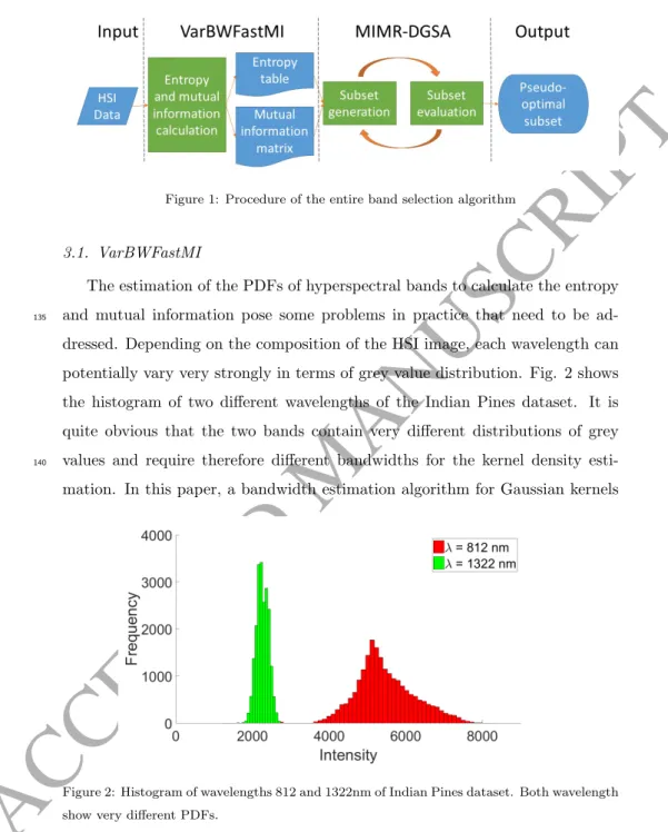
A flowchart of the proposed algorithm is outlined in Fig. 1, which has two main steps. The fast calculation of entropy and mutual information with

130

VarBWFastMI and MIMR-DGSA algorithm for band selection. Relevant details are presented in the following Sections.

ACCEPTED MANUSCRIPT

Figure 1: Procedure of the entire band selection algorithm

3.1. VarBWFastMI

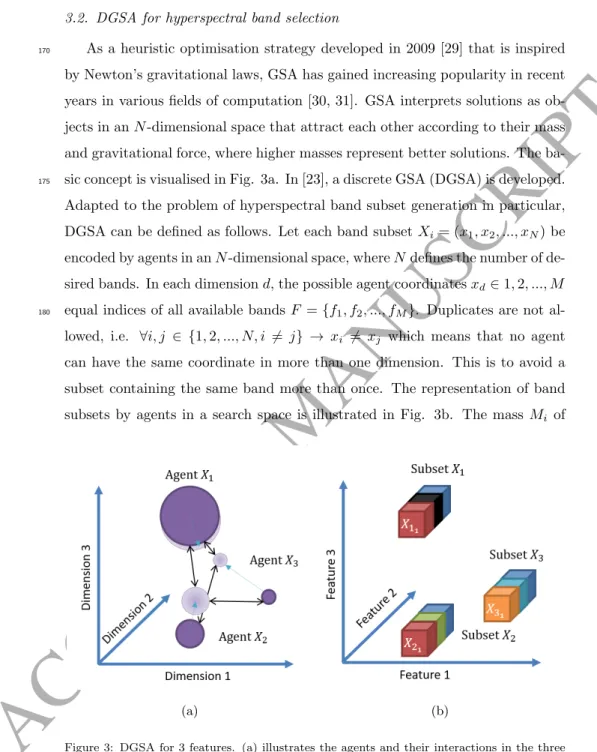
The estimation of the PDFs of hyperspectral bands to calculate the entropy and mutual information pose some problems in practice that need to be

ad-135

dressed. Depending on the composition of the HSI image, each wavelength can potentially vary very strongly in terms of grey value distribution. Fig. 2 shows the histogram of two different wavelengths of the Indian Pines dataset. It is quite obvious that the two bands contain very different distributions of grey values and require therefore different bandwidths for the kernel density

esti-140

mation. In this paper, a bandwidth estimation algorithm for Gaussian kernels

Figure 2: Histogram of wavelengths 812 and 1322nm of Indian Pines dataset. Both wavelength show very different PDFs.

ACCEPTED MANUSCRIPT

timation can be found in [27]. The bandwidth estimation can deliver a pseudo optimal bandwidth for each hyperspectral band and therefore generate better

145

estimates of the PDF and ultimately the entropy and mutual information. On the basis of the density estimate ˆph with a given bandwidthh, an

approxima-tion of the entropy H(X) of a band X with n sample points can be directly computed from: H(X) = n X i=1 ˆ ph(xi) log ˆph(xi) (7)

The calculation of the mutual information encounters additional challenges.

150

As seen in Eq. 2, the mutual information requires the joint entropy of the two random variables, which in turn requires a joint density estimate. Using a Gaussian kernel function, the joint density can be estimated by Eq. 5. The computational complexity however rises exponentially and for greater datasets, the cost for the mutual information calculation becomes impractical. In [24], a

155

fast algorithm for calculating the pairwise mutual information between features based on a Gaussian kernel density estimation is introduced for gene regulatory networks. The general idea is to use the fact that the integral of Eq. 2 can be approximated by the sample mean of the respective random variables. The proposed VarBWFastMI makes one major adjustment to that algorithm. Since

160

we estimate a different kernel bandwidth for each hyperspectral band, this needs to be considered for the pairwise mutual information calculation. Given the two bandwidthshxandhyfor the two bandsxand y, Eq. 5 can be rewritten as:

ˆ p(x, y) = 1 n n X i=1 1 p 2πhxhy ×exp −1 2 (x−xi)2 h2 x + (y−yi) 2 h2 y (8)

The algorithm in [24] can simply be adapted to estimate the joint densities by Eq. 8 to incorporate the variable bandwidths that are estimated. The

165

implementation of VarBWFastMI is based on the Matlab implementation of the fast pairwise mutual information available at [28]. The code is altered to incorporate variable bandwidths.

ACCEPTED MANUSCRIPT

As a heuristic optimisation strategy developed in 2009 [29] that is inspired

170

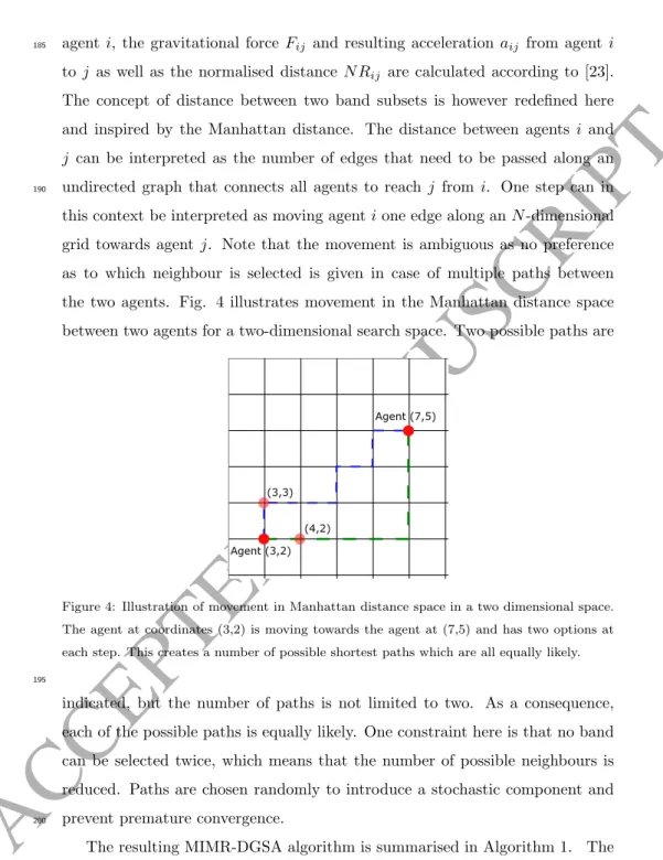
by Newton’s gravitational laws, GSA has gained increasing popularity in recent years in various fields of computation [30, 31]. GSA interprets solutions as ob-jects in anN-dimensional space that attract each other according to their mass and gravitational force, where higher masses represent better solutions. The ba-sic concept is visualised in Fig. 3a. In [23], a discrete GSA (DGSA) is developed.

175

Adapted to the problem of hyperspectral band subset generation in particular, DGSA can be defined as follows. Let each band subsetXi= (x1, x2, ..., xN) be

encoded by agents in anN-dimensional space, whereNdefines the number of de-sired bands. In each dimensiond, the possible agent coordinatesxd∈1,2, ..., M

equal indices of all available bandsF ={f1, f2, ..., fM}. Duplicates are not

al-180

lowed, i.e. ∀i, j ∈ {1,2, ..., N, i =6 j} → xi 6= xj which means that no agent

can have the same coordinate in more than one dimension. This is to avoid a subset containing the same band more than once. The representation of band subsets by agents in a search space is illustrated in Fig. 3b. The massMi of

(a) (b)

Figure 3: DGSA for 3 features. (a) illustrates the agents and their interactions in the three dimensional space and (b) the representation of band subsets through agents.

ACCEPTED MANUSCRIPT

agent i, the gravitational force Fij and resulting accelerationaij from agent i

185

to j as well as the normalised distance N Rij are calculated according to [23].

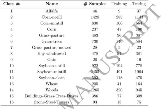
The concept of distance between two band subsets is however redefined here and inspired by the Manhattan distance. The distance between agents i and j can be interpreted as the number of edges that need to be passed along an undirected graph that connects all agents to reachj fromi. One step can in

190

this context be interpreted as moving agentione edge along anN-dimensional grid towards agent j. Note that the movement is ambiguous as no preference as to which neighbour is selected is given in case of multiple paths between the two agents. Fig. 4 illustrates movement in the Manhattan distance space between two agents for a two-dimensional search space. Two possible paths are

Figure 4: Illustration of movement in Manhattan distance space in a two dimensional space. The agent at coordinates (3,2) is moving towards the agent at (7,5) and has two options at each step. This creates a number of possible shortest paths which are all equally likely.

195

indicated, but the number of paths is not limited to two. As a consequence, each of the possible paths is equally likely. One constraint here is that no band can be selected twice, which means that the number of possible neighbours is reduced. Paths are chosen randomly to introduce a stochastic component and prevent premature convergence.

200

The resulting MIMR-DGSA algorithm is summarised in Algorithm 1. The initial populationP of agents is generated by a randmonised greedy initialisation where nc random bands out of all are selected as candidates and the one that

ACCEPTED MANUSCRIPT

Algorithm 1 MIMR-DGSA Algorithm

1: Input: nb: Number of desired bands;s: Size of population or number of

agents;itermax: Maximum number of iterations;nc: Number of candidates

for generation of initial population

2: Output: Best solutionPbestfound;

3: .Initialisation

4: iter←0;Kinit←s;Gstart←1;Gend←0

5: Generate initial populationP(iter) withsagents of lengthnb

6: Evaluate fitnessf iti= MIMR(Pi) and massMiof each agentPi∈P(iter)

7: .Main loop

8: whileiter < itermax do

9: UpdateG,K by linear reduction functions

10: UpdateKbestby selecting globalK best solutions

11: Calculate accelerationaijfor each agentPi∈P(iter) with respect to each

Pj∈Kbest 12: fori= 1 tosdo 13: Pi←Move(Pi, K, Kbest, aij). 14: end for 15: fori= 1 tosdo 16: Pi←LocalSearch(Pi) 17: end for 18: P(iter+ 1)←P(iter)

19: Evaluate fitnessf iti= MIMR(i) and massMiof each agentPi∈P(iter+

1)

20: Store best solutionPbest∈P(iter+ 1)∪Kbest

21: iter←iter+ 1

ACCEPTED MANUSCRIPT

produces the highest fitness is chosen and added to a set until the set reaches the desired sizenb. In the main loop, bothK and the gravitational constantGare

205

reduced by a linear reduction function. K should equal 1 in the last iteration. As suggested in [23], theKbest set contains the globally best agents out of all iterations instead of the local best agents of the current iteration. Mass and acceleration of each agent are calculated according to [23]. In the movement stage, it needs to be specified in which order theK best agents exert their force

210

onto other agents. As stated in [23], later movements have a more significant impact on the quality of the solution, which is why the priority is calculated by the inverse mass. At the end of each iteration, a local search is performed for each agent. This is based on the Hill climbing algorithm. The worst performing band of the current subset is replaced by the best performing band of all

re-215

maining bands, defined by the maximum entropy. The search terminates when no neighbour can improve the fitness of the subset. The algorithm terminates afteritermax iterations and the current best solution poses the pseudo-optimal

subset of selected bands.

4. Experimental Results

220

For performance assessment, the proposed MIMR-DGSA algorithm was tested on three different hyperspectral remote sensing datasets. Details of the datasets and comprehensive results are discussed in this section as follows.

4.1. Datasets and experimental setup

The three hyperspectral datasets include the Indian Pines, the Salinas and

225

the Pavia University. Matlab files for the used datasets can be found in [32]. The Indian Pines dataset was collected by the Airborne Visible/Infrared Imaging Spectrometer (AVIRIS)[33] in 1992 and is a subregion of an image covering the Indian Pines test site in North-western Indiana. It consists of 145×145 pixels and 224 spectral reflectance bands ranging from 400nm - 2500nm. It contains

230

two thirds agriculture and one third forest and other vegetation. The ground truth is divided in 16 classes as shown in Table 1.

ACCEPTED MANUSCRIPT

Table 1: Indian Pines dataset with ground truth classes and their description as well as number of samples available in each class

Class # Name # Samples Training Testing

1 Alfalfa 46 9 37 2 Corn-notill 1428 285 1143 3 Corn-mintill 830 166 664 4 Corn 237 47 190 5 Grass-pasture 483 96 387 6 Grass-trees 730 146 584 7 Grass-pasture-mowed 28 5 23 8 Hay-windrowed 478 97 381 9 Oats 20 4 16 10 Soybean-notill 972 194 778 11 Soybean-mintill 2455 491 1964 12 Soybean-clean 593 118 475 13 Wheat 205 41 164 14 Woods 1265 320 945 15 Buildings-Grass-Trees-Drives 386 77 309 16 Stone-Steel-Towers 93 18 75

The Salinas dataset was also collected by the AVIRIS sensor over the Salinas Valley, California. The dataset comprises 512×217 pixels and again 224 bands and has therefore a significantly higher data amount than the Indian Pines

235

scene. The scene depicts vegetables, bare soils, and vineyard fields. The ground truth also contains 16 classes, depicted in Fig. 2. To reduce noise effects in the data, the water absorption band regions were removed, i.e. bands [104 - 108], [150 - 163] and 220 for both the Salinas and Indian Pines datasets.

The Pavia University dataset was acquired by the Reflective Optics System

240

Imaging Spectrometer (ROSIS)[34] during a flight campaign over Pavia, North-ern Italy. It consists of 610 × 610 samples and 103 spectral bands covering a range within 430nm - 860nm. As shown in Fig. 3, the ground truth contains 9 classes.

To evaluate the performance of the proposed MIMR-DGSA algorithm, it was

ACCEPTED MANUSCRIPT

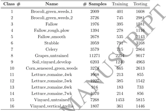
Table 2: Salinas dataset with ground truth classes and their description as well as number of samples available in each class

Class # Name # Samples Training Testing

1 Brocoli green weeds 1 2009 401 1608 2 Brocoli green weeds 2 3726 745 2981 3 Fallow 1976 395 1581 4 Fallow rough plow 1394 278 1116 5 Fallow smooth 2678 535 2143 6 Stubble 3959 791 3168 7 Celery 3579 715 2864 8 Grapes untrained 11271 2254 9017 9 Soil vinyard develop 6203 1240 4963 10 Corn senesced green weeds 3278 665 2613 11 Lettuce romaine 4wk 1068 213 855 12 Lettuce romaine 5wk 1927 385 1542 13 Lettuce romaine 6wk 916 183 733 14 Lettuce romaine 7wk 1070 214 856 15 Vinyard untrained 7268 1453 5815 16 Vinyard vertical trellis 1807 361 1446

Table 3: Pavia University dataset with ground truth classes and their description as well as number of samples available in each class

Class # Name # Samples Training Testing

1 Asphalt 6631 1326 5305 2 Meadows 18649 3729 14920 3 Gravel 2099 419 1680 4 Trees 3064 612 2452 5 Painted metal sheets 1345 269 1076 6 Bare Soil 5029 1005 4024 7 Bitumen 1330 266 1064 8 Self-Blocking Bricks 3682 736 2946 9 Shadows 947 186 761

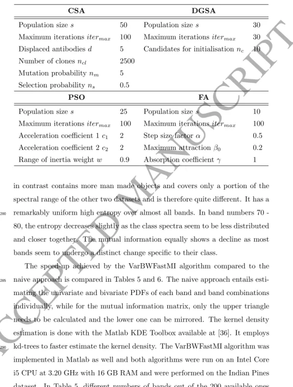
compared with the original CSA version as well as PSO and FA. The individual parameter settings are listed in Table 4. For CSA, the settings are based on [6],

ACCEPTED MANUSCRIPT

whereas for PSO and FA, the parameters of the respective literature were used as a basis and were empirically adjusted for optimal results on the data used in this paper. All algorithms are compared with respect to their band selection

250

capabilities and time consumption. The band selection capabilities were assessed with respect to pixel-wise classification. A Support Vector Machine (SVM) with a Radial Basis Function (RBF) kernel whose parameters C andγwere tuned by a grid search, i.e. selecting 20% of the pixels of each dataset’s classes randomly for training and the remaining 80% for validation. The test- and validation-set

255

splitting was repeated 10 times for each dataset and 3 runs of each algorithm were performed for each set making it 30 runs per dataset. As a state-of-the-art unsupervised feature selection benchmark for the classification performance, Ward’s Linkage strategy using Mutual Information (WaLuMI)[35] algorithm was applied. It hierarchically groups the spectral bands by a distance measure based

260

on mutual information and selects a representative of each group as the band subset. WaLuMI was chosen as it performs best among all compared algorithms in [6] and therefore serves as a baseline. To compare the performance of the MIMR criterion, the Fuzzy C-Means clustering method (FCM) has also been applied in combination with DGSA and ultimately, a classification using all

265

bands of each dataset was compared with that of the selected features.

4.2. Entropy and mutual information

For each of the three datasets, the lookup tables for the entropy and mu-tual information were calculated with the proposed VarBWFastMI algorithm. Results are visualised in Fig. 10 along the class mean spectra of each class in

270

all three datasets. As expected, the Indian Pines and Salinas datasets show a strong structural similarity for both the entropy and mutual information as they are captured with the same sensor and contain similar vegetation scenes. The bands on the edges of the water absorption regions in the Indian Pines and Salinas datasets show a very low entropy and a low mutual information with

275

the rest of the bands. Wavelength numbers 40 - 100 seem to carry the most information as the entropy is the highest in that range. The Pavia University

ACCEPTED MANUSCRIPT

Table 4: Parameter configurations for the different algorithms

CSA DGSA

Population sizes 50 Population sizes 30 Maximum iterationsitermax 100 Maximum iterationsitermax 30

Displaced antibodiesd 5 Candidates for initialisation nc 10

Number of clonesncl 2500

Mutation probabilitynm 5

Selection probabilityns 0.5

PSO FA

Population sizes 25 Population sizes 10 Maximum iterationsitermax 100 Maximum iterationsitermax 100

Acceleration coefficient 1c1 2 Step size factor α 0.5

Acceleration coefficient 2c2 2 Maximum attractionβ0 0.2

Range of inertia weightw 0.9 Absorption coefficientγ 1

in contrast contains more man made objects and covers only a portion of the spectral range of the other two datasets and is therefore quite different. It has a remarkably uniform high entropy over almost all bands. In band numbers 70

-280

80, the entropy decreases slightly as the class spectra seem to be less distributed and closer together. The mutual information equally shows a decline as most bands seem to undergo a distinct change specific to their class.

The speed-up achieved by the VarBWFastMI algorithm compared to the naive approach is compared in Tables 5 and 6. The naive approach entails

esti-285

mating the univariate and bivariate PDFs of each band and band combinations individually, while for the mutual information matrix, only the upper triangle needs to be calculated and the lower one can be mirrored. The kernel density estimation is done with the Matlab KDE Toolbox available at [36]. It employs kd-trees to faster estimate the kernel density. The VarBWFastMI algorithm was

290

implemented in Matlab as well and both algorithms were run on an Intel Core i5 CPU at 3.20 GHz with 16 GB RAM and were performed on the Indian Pines dataset. In Table 5, different numbers of bands out of the 200 available ones

ACCEPTED MANUSCRIPT

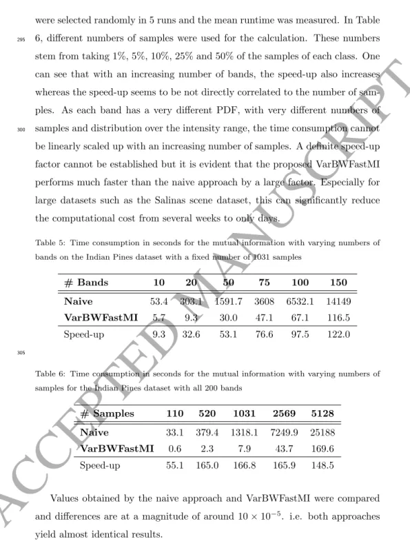
were selected randomly in 5 runs and the mean runtime was measured. In Table 6, different numbers of samples were used for the calculation. These numbers

295

stem from taking 1%, 5%, 10%, 25% and 50% of the samples of each class. One can see that with an increasing number of bands, the speed-up also increases whereas the speed-up seems to be not directly correlated to the number of sam-ples. As each band has a very different PDF, with very different numbers of samples and distribution over the intensity range, the time consumption cannot

300

be linearly scaled up with an increasing number of samples. A definite speed-up factor cannot be established but it is evident that the proposed VarBWFastMI performs much faster than the naive approach by a large factor. Especially for large datasets such as the Salinas scene dataset, this can significantly reduce the computational cost from several weeks to only days.

Table 5: Time consumption in seconds for the mutual information with varying numbers of bands on the Indian Pines dataset with a fixed number of 1031 samples

# Bands 10 20 50 75 100 150

Naive 53.4 303.1 1591.7 3608 6532.1 14149

VarBWFastMI 5.7 9.3 30.0 47.1 67.1 116.5 Speed-up 9.3 32.6 53.1 76.6 97.5 122.0

305

Table 6: Time consumption in seconds for the mutual information with varying numbers of samples for the Indian Pines dataset with all 200 bands

# Samples 110 520 1031 2569 5128

Naive 33.1 379.4 1318.1 7249.9 25188

VarBWFastMI 0.6 2.3 7.9 43.7 169.6 Speed-up 55.1 165.0 166.8 165.9 148.5

Values obtained by the naive approach and VarBWFastMI were compared and differences are at a magnitude of around 10×10−5_{. i.e. both approaches}

ACCEPTED MANUSCRIPT

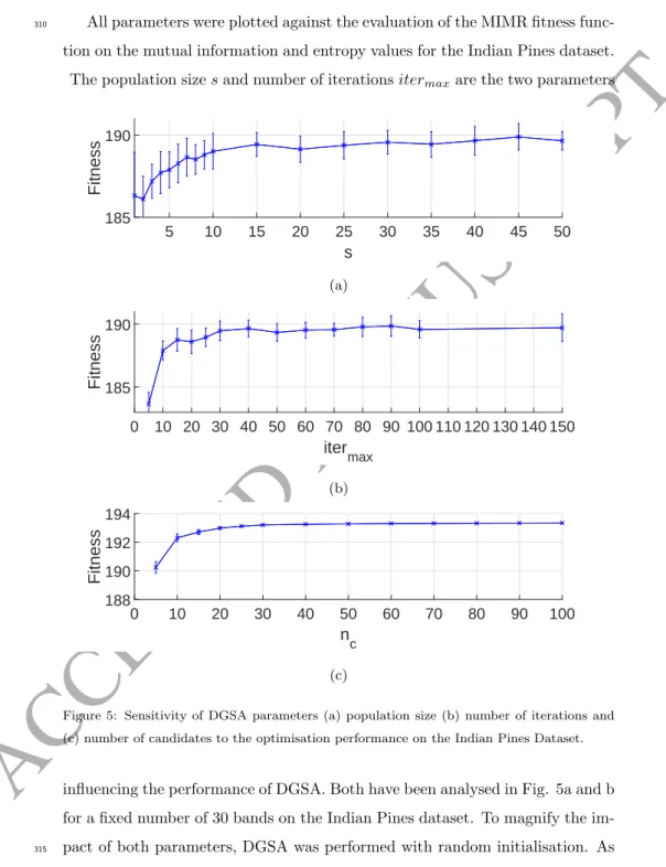
All parameters were plotted against the evaluation of the MIMR fitness

func-310

tion on the mutual information and entropy values for the Indian Pines dataset. The population sizesand number of iterationsitermaxare the two parameters

5 10 15 20 25 30 35 40 45 50 s 185 190 Fitness (a) 0 10 20 30 40 50 60 70 80 90 100 110 120 130 140 150 iter max 185 190 Fitness (b) 0 10 20 30 40 50 60 70 80 90 100 n c 188 190 192 194 Fitness (c)

Figure 5: Sensitivity of DGSA parameters (a) population size (b) number of iterations and (c) number of candidates to the optimisation performance on the Indian Pines Dataset.

influencing the performance of DGSA. Both have been analysed in Fig. 5a and b for a fixed number of 30 bands on the Indian Pines dataset. To magnify the im-pact of both parameters, DGSA was performed with random initialisation. As

ACCEPTED MANUSCRIPT

expected, both parameters increase the performance by increasing their values. They are chosen to be as minimal as possible to achieve maximum optimisa-tion capacity with minimal computaoptimisa-tional effort. Based on these results,sand itermaxare both set to 30 in future experiments for our MIMR-DGSA method.

The number of candidatesnc for the initialisation was analysed in Fig. 5c.

320

By increasing this number, the chances of picking a good solution increase as well. However, to guarantee a good exploration of the search space, a trade-off between subset fitness and population diversity is mandatory. Therefore, we suggest to setnc to 10.

4.4. Runtime analysis 325

As stated in [20], MIMR-PSO has a computational complextity ofO(i×s×

n2

b) which is linearly correlated to the number of iterationsi, the population size

sand quadratically correlated to the number of desired bandsnbcaused by the

MIMR evaluation. Due to the interaction between the fireflies in MIMR-FA, it is quadratically correlated to the size of the population and has a complexity

330

of O(i×s2 _×n2

b). As stated in [6], MIMR-CSA has a time complexity of

O(i×ncl×n2b), which is linearly dependent on the number of clones ncl and

quadratically dependent on the number of selected bands nb. MIMR-DGSA

also has a quadratic complexity, i.e. O(i×s×K×n2

b), but the number of

MIMR evaluations per iterations is limited to the number of initial agentssand

335

the decreasing number of K best solutions. The initialisation of DGSA has a time complexity ofO(s×nc×n2b), which is linearly correlated to the number

of candidatesnc and quadratically correlated to nb. All algorithms share the

dependence on number of iteration and the quadratic runtime of the MIMR evaluation, showing the importance of pre-calculating the entropy and mutual

340

information. The main differences are rooted in the population size and the interaction between the solutions. MIMR-DGSA has an additional initialisation step which can potentially decrease the efficiency. In our, case, the number of candidates for the initialisation is relatively low, which is why this step does not have a big effect on the runtime.

ACCEPTED MANUSCRIPT

MIMR-CSA, s = 50, iter_max = 100

MIMR-DGSA, s = 50, iter_max = 100

MIMR-DGSA, s = 30, iter_max = 30

MIMR-PSO, s = 25, iter

max = 100

MIMR-FA, s = 10, iter_max = 100

(a) 0 10 20 30 40 50 60 70 80 90 100 Number of bands 0 0.5 1 1.5 2 Time (s) (b)

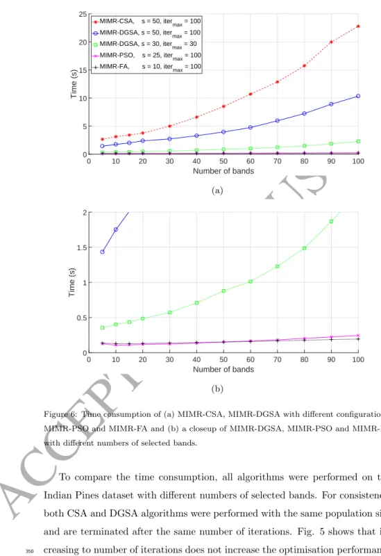
Figure 6: Time consumption of (a) MIMR-CSA, MIMR-DGSA with different configurations, MIMR-PSO and MIMR-FA and (b) a closeup of MIMR-DGSA, MIMR-PSO and MIMR-FA with different numbers of selected bands.

To compare the time consumption, all algorithms were performed on the Indian Pines dataset with different numbers of selected bands. For consistency, both CSA and DGSA algorithms were performed with the same population size and are terminated after the same number of iterations. Fig. 5 shows that in-creasing to number of iterations does not increase the optimisation performance

ACCEPTED MANUSCRIPT

significantly. Additionally, MIMR-DGSA was performed with optimised popula-tion size and iterapopula-tions, as established in Secpopula-tion 4.3. The number of candidates for the initialisation of DGSA is set to 10. For PSO and FA, the population size and iterations were set according to [20] and [21] respectively and slightly adjusted based on empirical values and all other parameters are set as specified

355

in Table 4. As seen from the time measurements in Fig. 6, MIMR-DGSA with the samesanditermaxas MIMR-CSA performs about twice as fast. With the

parameter settings established in Section 4.3, MIMR-DGSA only requires a frac-tion of the time of MIMR-CSA, where for 150 features, MIMR-DGSA takes only 5 seconds compared to over 50 seconds for MIMR-CSA. The increased time

con-360

sumption of CSA is rooted in the relatively high number of clones per antigen, whereas DGSA only has a limited number of agents with a decreasing number ofK best agents. PSO and FA both perform very similar and both outperform CSA and DGSA due to their straightforward implementation of the movement strategy. DGSA suffers in this respect due to the elaborate neighbourhood and

365

movement concept.

4.5. Classification performance

In this subsection, the classification accuracy using the selected features are compared to evaluate the efficacy of the band selection approaches. MIMR-FA, MIMR-PSO, MIMR-CSA, MIMR-DGSA as well as WaLuMI were performed

370

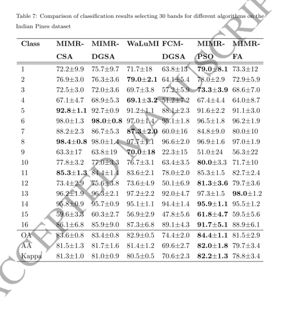
selecting 30 bands on the Indian Pines and Salinas datasets and 20 bands on the Pavia University dataset. The Overall Accuracy (OA), Average Accuracy (AA) and Kappa coefficient were calculated in every case alongside the individual class accuracies. Results are summarised in Tables 7, 8 and 9 for comparison.

As seen in Table 7, in terms of OA, MIMR-PSO performs best for 30 bands on

375

the Indian Pines dataset, where MIMR-CSA and MIMR-DGSA perform roughly similar. Only FCM-DGSA performs significantly worse. Looking at Fig. 7, One can see that MIMR-DGSA and MIMR-CSA also perform very similar for differ-ent numbers of selected bands, outperforming MIMR-FA and WaLuMI, whereas MIMR-PSO performs best selecting 90 or less bands. For the Salinas dataset,

ACCEPTED MANUSCRIPT

Table 7: Comparison of classification results selecting 30 bands for different algorithms on the Indian Pines dataset

Class MIMR-CSA MIMR-DGSA WaLuMI FCM-DGSA MIMR-PSO MIMR-FA 1 72.2±9.9 75.7±9.7 71.7±18 63.8±13 79.0±8.1 73.3±12 2 76.9±3.0 76.3±3.6 79.0±2.1 64.1±5.4 78.0±2.9 72.9±5.9 3 72.5±3.0 72.0±3.6 69.7±3.8 57.2±5.9 73.3±3.9 68.6±7.0 4 67.1±4.7 68.9±5.3 69.1±3.2 51.2±7.2 67.4±4.4 64.0±8.7 5 92.8±1.1 92.7±0.9 91.2±1.1 88.1±2.3 91.6±2.2 91.1±3.0 6 98.0±1.3 98.0±0.8 97.0±1.4 95.1±1.8 96.5±1.8 96.2±1.9 7 88.2±2.3 86.7±5.3 87.3±2.0 60.0±16 84.8±9.0 80.0±10 8 98.4±0.8 98.0±1.4 97.7±1.1 96.6±2.0 96.9±1.6 97.0±1.9 9 63.3±17 63.8±19 70.0±18 22.3±15 51.0±24 56.3±22 10 77.8±3.2 77.0±3.3 76.7±3.1 63.4±3.5 80.0±3.3 71.7±10 11 85.3±1.3 84.4±1.4 83.6±2.1 78.0±2.0 85.3±1.5 82.7±2.4 12 73.4±2.9 75.6±3.8 73.6±4.9 50.1±6.9 81.3±3.6 79.7±3.6 13 96.2±1.9 96.3±2.1 97.2±2.2 92.0±4.7 97.3±1.5 98.0±1.2 14 95.8±0.9 95.7±0.9 95.1±1.1 94.4±1.4 95.9±1.1 95.5±1.2 15 59.6±3.3 60.3±2.7 56.9±2.9 47.8±5.6 61.8±4.7 59.5±5.6 16 86.1±6.8 85.9±9.0 87.3±6.8 89.1±4.3 91.7±5.1 88.9±6.1 OA 83.6±0.8 83.4±0.8 82.9±0.5 74.4±2.0 84.4±1.1 81.5±2.9 AA 81.5±1.3 81.7±1.6 81.4±1.2 69.6±2.7 82.0±1.8 79.7±3.4 Kappa 81.3±1.0 81.0±0.9 80.5±0.5 70.6±2.3 82.2±1.3 78.8±3.4

ACCEPTED MANUSCRIPT

Table 8: Comparison of classification results selecting 30 bands for different algorithms on the Salinas dataset Class MIMR-CSA MIMR-DGSA WaLuMI FCM-DGSA MIMR-PSO MIMR-FA 1 99.5±0.2 99.5±0.2 99.4±0.2 99.5±0.4 99.4±0.4 99.4±0.4 2 99.8±0.2 99.8±0.2 99.8±0.1 99.8±0.1 99.8±0.1 99.7±0.2 3 98.6±0.4 98.8±0.4 99.6±0.2 99.3±0.4 99.3±0.4 99.2±0.5 4 99.4±0.2 99.4±0.3 99.5±0.2 99.2±0.4 99.3±0.4 99.4±0.4 5 98.2±0.4 98.4±0.6 99.0±0.4 98.9±0.5 98.9±0.4 98.8±0.6 6 99.8±0.1 99.8±0.1 99.9±0.1 99.9±0.1 99.8±0.1 99.8±0.1 7 99.8±0.1 99.8±0.1 99.7±0.1 99.6±0.2 99.6±0.2 99.6±0.2 8 87.5±0.8 88.3±0.9 88.6±0.5 88.8±0.6 88.8±0.7 89.2±0.6 9 98.4±0.4 99.2±0.7 99.8±0.2 99.7±0.1 99.8±0.1 99.8±0.1 10 94.8±0.6 95.6±0.8 97.3±0.6 96.6±0.9 97.2±0.6 97.3±0.6 11 92.7±1.6 96.1±2.5 98.8±0.4 98.3±0.9 98.4±1.0 99.0±0.7 12 99.8±0.2 99.8±0.2 99.8±0.1 99.9±0.1 99.8±0.4 99.9±0.1 13 99.4±0.3 99.5±0.3 98.9±0.6 99.1±0.6 99.2±0.5 99.2±0.5 14 97.7±1.0 97.9±0.9 97.1±1.0 97.4±1.3 97.4±1.3 98.0±1.2 15 71.5±1.4 74.3±2.3 73.6±1.1 75.2±1.3 74.6±2.6 75.8±2.2 16 99.1±0.2 99.1±0.2 98.9±0.2 98.8±0.3 98.8±0.3 98.9±0.3 OA 92.6±0.3 93.4±0.5 93.6±0.1 93.8±0.2 93.8±0.4 94.0±0.4 AA 96.0±0.2 96.6±0.4 96.9±0.1 96.9±0.2 96.9±0.3 97.1±0.3 Kappa 91.8±0.3 92.6±0.6 92.9±0.1 93.1±0.3 93.0±0.5 93.3±0.4

ACCEPTED MANUSCRIPT

Table 9: Comparison of classification results selecting 20 bands for different algorithms on the Pavia University dataset

Class MIMR-CSA MIMR-DGSA WaLuMI FCM-DGSA MIMR-PSO MIMR-FA 1 92.2±0.6 92.1±1.0 92.9±0.4 90.3±1.2 91.7±1.4 93.5±0.8 2 97.9±0.2 97.7±0.2 96.9±0.2 96.5±0.5 97.0±0.5 97.1±0.5 3 75.3±1.7 74.7±3.7 76.0±1.0 66.8±6.9 74.9±5.1 77.4±3.3 4 94.1±0.8 93.8±0.9 91.5±0.7 90.4±1.1 92.3±1.2 92.7±1.4 5 99.3±0.3 99.4±0.3 99.3±0.2 98.5±0.6 99.1±0.3 99.2±0.3 6 89.6±0.6 88.4±1.1 81.1±1.1 64.6±9.9 77.4±9.0 83.0±5.5 7 78.7±1.8 78.0±3.4 80.9±1.7 80.2±2.1 82.2±1.9 83.8±1.7 8 87.4±0.9 87.6±1.6 87.9±0.7 86.8±1.8 88.7±1.6 89.8±1.1 9 99.9±0.2 99.9±0.1 99.8±0.2 99.7±0.2 99.8±0.1 99.8±0.2 OA 93.2±0.1 92.9±0.5 91.9±0.1 88.7±1.8 91.4±1.7 92.7±1.1 AA 90.5±0.3 90.2±0.9 89.6±0.2 86.0±2.2 89.2±1.9 90.7±1.2 Kappa 91.0±0.2 90.6±0.7 89.2±0.1 84.8±2.5 88.5±2.3 90.3±1.5

Table 10: Mean OA, AA and Kappa Coefficient over the three datasets of the different algo-rithms. MIMR-CSA MIMR-DGSA WaLuMI FCM-DGSA MIMR-PSO MIMR-FA OA 89.80±0.4089.90±0.6089.47±0.23 85.63±1.33 89.87±1.07 89.40±1.47 AA 89.33±0.6089.50±0.9789.30±0.50 84.17±1.70 89.37±1.33 89.17±1.63 Kappa 88.03±0.5088.07±0.7387.53±0.23 82.83±1.70 87.90±1.37 87.47±1.77

ACCEPTED MANUSCRIPT

MIMR-FA performs best as seen in Table 8 and Fig. 8. Again MIMR-CSA and MIMR-DGSA show a very similar performance for different numbers of bands but are outperformed by WaLuMI and notably FCM-DGSA for a lower number of bands. For the Pavia University dataset, MIMR in combination with CSA, DGSA, FA and PSO all outperform WaLuMI and FCM-DGSA for any number

385

of bands up to 75, as seen in Fig. 9 where CSA seems to perform best selecting 20 bands. Both MIMR-DGSA and MIMR-CSA again perform very similar as shown in Table 9 and Fig. 9. Another observation that can be made specifically from Tables 7 and 9 is that MIMR-PSO and MIMR-FA yield a larger standard deviation. This might hint at the fact that they have less optimisation

qual-390

ities for the MIMR criterion and the selected bands are more random, which is examined in Section 4.6. Even though this yields higher mean accuracy, the algorithms are less reliable in individual runs. This leads to the conclusion that FA and PSO can potentially achieve a higher classification accuracy in indi-vidual cases, whereas CSA and DGSA perform slightly less but more robust

395

for different datasets. None of the presented algorithms consistently generates optimal performance. To investigate this, we have compared the average mea-sures of the OA, AA and Kappa coefficient over the three datasets, as shown in Table 10. MIMR-DGSA seems to slightly outperform all other algorithms. This hints at the fact that DGSA performs better in terms of generalising over

400

different datasets, but in individual cases, might perform inferior. Hence, even though FA and PSO may produce higher classification accuracy in individual cases, their overall performance for band selection can be compromised due to inferior generalisation capabilities. This is evaluated in detail in the following section.

405

4.6. Optimisation performance

In this section, we are investigating the optimisation performance of the EAs with respect to the MIMR criterion. The objective is to maximise the individual entropies of selected bands and minimise their mutual information. A higher MIMR value indicates a better subset. The actual value is dependent on the

ACCEPTED MANUSCRIPT

0

25

50

75

100

125

150

Number of bands

60

70

80

90

OA

Figure 7: Performance comparison of all band selection algorithms on the Indian Pines dataset

0

25

50

75

100

125

150

Number of bands

88

90

92

94

96

OA

Figure 8: Performance comparison of all band selection algorithms on the Salinas dataset

constitution of each dataset, but algorithms can be compared among each other within one dataset. Table 11 summarises the mean MIMR value achieved after the last iteration of the four EAs of 20 runs. One can see that FA performs worst on all datasets, whereas CSA and DGSA perform very similar. PSO performs better than FA and even becomes even with DGSA for the Pavia

Uni-415

versity dataset but worse for the other datasets. As seen in Fig. 11, the mutual information and especially the entropy for most bands in the Pavia University

ACCEPTED MANUSCRIPT

0

25

50

75

Number of bands

75

80

85

90

95

OA

Figure 9: Performance comparison of all band selection algorithms on the Pavia University dataset

Table 11: Comparison of optimisation performance of the different optimisation algorithms. Values indicate the evaluation of the MIMR criterion of the best solution achieved by each optimisation algorithm.

Dataset # Bands FA PSO CSA DGSA

Indian Pines 30 175 188 193 193

Salinas 30 159 168 173 172 Pavia University 20 138 141 141 141

dataset are very similar which might suggest that most band combinations yield similar MIMR values. This explains why the optimisation performance of all algorithms is very similar. These findings confirm the above assumption that

420

optimising the MIMR criterion does not necessarily imply an optimal classifi-cation accuracy. However, better optimisation of the MIMR criterion results in a more robust accuracy and therefore band selection performance. The fact that FA and PSO yield a better classification accuracy with an inferior optimi-sation capability of the chosen MIMR criterion hence exposes shortcomings of

425

the criterion rather than a superior band selection quality of the optimisation algorithm. For this reason, we consider both CSA and DGSA as more suitable for the proposed task.

ACCEPTED MANUSCRIPT

50 100 150 200 Bandnumber 50 100 150 200 Bandnumber (a) 50 100 150 200 Bandnumber 50 100 150 200 Bandnumber (b) 50 100 150 200 Bandnumber 4 6 8 Entropy (c) 50 100 150 200 Bandnumber 4 6 8 Entropy (d) 20 40 60 80 100 120 140 160 180 200 Bandnumber 2000 4000 6000 8000 Intensity (e) 50 100 150 200 Bandnumber 0 2000 4000 6000 8000 Intensity (f)

Figure 10: Comparison of (a) - (b) mutual information, (c) - (d) entropy and (e) - (f) selected bands with DGSA where (a), (c) and (e) refer to the Indian Pines and (b), (d) and (f) to the Salinas dataset. The selected bands could achieve 83.7% OA for Indian Pines and 92.6 % for Salinas

To verify the selected bands of MIMR-DGSA, the bands of a representative

430

run were plotted on top of the mean spectra of each class in all datasets in Fig. 10 and 11 alongside the mutual information matrices and entropy tables. For the Indian Pines dataset, bands 14 16, 20, 23, 26, 29, 31, 34 39, 41, 43

-ACCEPTED MANUSCRIPT

Figure 11: Comparison of (a) mutual information, (b) entropy and (c) selected bands with DGSA of the Pavia University dataset with an OA of 93.5%.

45, 49, 54, 62, 63, 65, 68, 71, 84 - 86, 99 and 117 were selected. In the Salinas dataset, bands 1, 3 - 5, 11, 13, 20, 21, 25, 33 - 35, 37 - 42, 45, 47, 49, 51, 52,

435

55, 68, 74, 76, 91, 93 and 94 were selected and for the Pavia University dataset, only 20 bands were selected, i.e. 1 - 6, 19, 39, 49, 63, 69, 72, 74, 76, 78, 83, 91, 100, 102 and 103. The bands indexed from 40 to 100 in both the Indian Pines and Salinas scene have the highest entropy and equally a relatively low mutual information with other regions. Looking at the spectra, this region seems to

ACCEPTED MANUSCRIPT

show the biggest differences between the classes, justifying why most bands are selected in this area in both datasets. The bands edging the water absorption regions have a low mutual information but also a very low entropy, which is why they are not selected. The bands higher than 120 have a relatively high entropy but also a quite high mutual information with adjacent bands over a

445

larger region. This is likely the reason why they are hardly ever selected. The mean spectra seem to be very similar in this region as well for most classes. The Pavia University dataset contains the most differences between the classes in the exact wavelength region around number 70, with a slightly lower entropy but also a much lower mutual information with all other regions. This makes the

450

corresponding region most significant for classification. The edges of all spectra also show some changes in the shapes and are therefore selected. The rest of the bands seem to be evenly distributed over the spectral range.

5. Conclusion

In this paper, the MIMR-DGSA algorithm was proposed for hyperspectral

455

band selection. The algorithm is based on the MIMR criterion aiming to max-imise the entropy of bands and minmax-imise the mutual information between the bands in a subset. To evaluate the criterion, the entropy and mutual informa-tion are pre-calculated. A detailed analysis of the calculainforma-tion of these measures for hyperspectral bands was presented resulting in the VarBWFastMI algorithm

460

that calculates the pairwise mutual information of hyperspectral datasets in a reasonable amount of time and incorporates variable bandwidths for the density estimation. Additionally, a modified DGSA is developed introducing a neigh-bourhood and movement concept for feature subsets in a discrete optimisation space that generates potential subsets in a heuristic way and eventually

gener-465

ates a pseudo-optimal solution. Results on three publicly available HSI remote sensing datasets show that the proposed MIMR-DGSA performs very similar to the original MIMR-CSA, on which it is based, but is much faster and easier to use, as it only has three parameters. Parameters for the number of agents and

ACCEPTED MANUSCRIPT

iterations are directly correlated with the quality of the optimisation, whereas

470

the number of candidates for the initialisation requires individual tuning based on the underlying dataset.

When comparing both CSA and DGSA with other EAs, we were able to show that FA and PSO are both less suitable to optimise the MIMR criterion. The effect of this is that the achieved classification accuracy is subject to high

475

variance. While PSO and FA can achieve a higher accuracy in individual cases, DGSA was shown to perform superior and be more robust in average over all datasets. This also lead us to conclude that the MIMR criterion itself does not necessarily optimise classification accuracy. In other applications such as regression or object detection, optimising the MIMR criterion might however

480

perform better. Furthermore, PSO and FA require almost as many parameters as CSA and need therefore additional tuning. None of the examined algorithms performs consistently best in terms of accuracy, however, DGSA poses a robust, faster and easier to use alternative to CSA, which both optimise the MIMR criterion best. In combination with VarBWFastMI, we have therefore proposed

485

an efficient state-of-the-art band selection algorithm. In future work, a more robust and faster converging DGSA will be explored, and the conjecture that MIMR performs well for applications other than classification will be examined in detail.

Acknowledgements

490

This project is partially funded by Engineering the Future (ETF) Schol-arship, Faculty of Engineering, University of Strathclyde; DSTL (R-CLOUD contract DSTLX-1000103251/1000098854); the Fundamental Research Funds for the Central Universities (18CX05030A); Guangdong Provincial Application-oriented Technical Research and Development Special Fund Project

495

ACCEPTED MANUSCRIPT

References

[1] J. Zabalza, J. Ren, J. Zheng, J. Han, H. Zhao, S. Li, S. Marshall, Novel Two-Dimensional Singular Spectrum Analysis for Effective Feature

Extrac-500

tion and Data Classification in Hyperspectral Imaging, IEEE Trans. Geosci. Remote Sens. 53 (8) (2015) 4418–4433.

[2] T. Qiao, Z. Yang, J. Ren, P. Yuen, H. Zhao, G. Sun, S. Marshall, J. A. Benediktsson, Joint bilateral filtering and spectral similarity-based sparse representation: A generic framework for effective feature extraction and

505

data classification in hyperspectral imaging, Pattern Recognit. (2018) 316 – 328.

[3] X. Lu, W. Zhang, X. Li, A Hybrid Sparsity and Distance-Based Discrimina-tion Detector for Hyperspectral Images, IEEE TransacDiscrimina-tions on Geoscience and Remote Sensing 56 (3) (2018) 1704–1717.

510

[4] J. Zabalza, J. Ren, J. Zheng, H. Zhao, C. Qing, Z. Yang, P. Du, S. Mar-shall, Novel segmented stacked autoencoder for effective dimensionality re-duction and feature extraction in hyperspectral imaging, Neurocomputing 185 (2016) 1–10.

[5] Y. Saeys, I. Inza, P. Larra˜naga, A review of feature selection techniques in

515

bioinformatics, Bioinformatics 23 (19) (2007) 2507–2517.

[6] J. Feng, L. Jiao, F. Liu, T. Sun, X. Zhang, Unsupervised feature selection based on maximum information and minimum redundancy for hyperspec-tral images, Pattern Recognit. 51 (2016) 295–309.

[7] H. G. Vijouyeh, G. Taskin, A comprehensive evaluation of feature

selec-520

tion algorithms in hyperspectral image classification, in: 2016 IEEE Int. Geoscience and Remote Sensing Symp. (IGARSS), 2016, pp. 489–492.

ACCEPTED MANUSCRIPT

[8] Y. Liu, Y. Chen, K. Tan, H. Xie, L. Wang, X. Yan, W. Xie, Z. Xu, Max-imum relevance, minMax-imum redundancy band selection based on neighbor-hood rough set for hyperspectral data classification, Meas. Sci. Technol.

525

27 (12) (2016) 125501.

[9] G. Taskin, H. Kaya, L. Bruzzone, Feature selection based on high dimen-sional model representation for hyperspectral images, IEEE Trans. Image Process. 26 (6) (2017) 2918–2928.

[10] P. Bajcsy, P. Groves, Methodology for Hyperspectral Band Selection,

Pho-530

togramm. Eng. & Remote Sensing 70 (7) (2004) 793–802.

[11] R. Yang, L. Su, X. Zhao, H. Wan, J. Sun, Representative band selection for hyperspectral image classification, J. Vis. Commun. Image Represent. 48 (2017) 396–403.

[12] M. Zhang, J. Ma, M. Gong, Unsupervised Hyperspectral Band Selection by

535

Fuzzy Clustering With Particle Swarm Optimization, IEEE Geosci. Remote Sens. Lett. 14 (5) (2017) 773–777.

[13] X. Luo, R. Xue, J. Yin, Information-Assisted Density Peak Index for Hy-perspectral Band Selection, IEEE Geosci. Remote Sens. Lett. 14 (10) (2017) 1870–1874.

540

[14] Q. Du, H. Yang, Similarity-Based Unsupervised Band Selection for Hy-perspectral Image Analysis, IEEE Geosci. Remote Sens. Lett. 5 (4) (2008) 564–568.

[15] E. Amaldi, V. Kann, On the approximability of minimizing nonzero vari-ables or unsatisfied relations in linear systems, Theor. Comput. Sci. 209 (1)

545

(1998) 237–260.

[16] Y. Liu, G. Wang, H. Chen, H. Dong, X. Zhu, S. Wang, An improved particle swarm optimization for feature selection, Journal of Bionic Engineering 8 (2) (2011) 191–200.

ACCEPTED MANUSCRIPT

[17] B. Xue, M. Zhang, W. N. Browne, Particle swarm optimization for feature

550

selection in classification: A multi-objective approach, IEEE Transactions on Cybernetics 43 (6) (2013) 1656–1671.

[18] E. Emary, H. M. Zawbaa, K. K. A. Ghany, A. E. Hassanien, B. Parv, Firefly Optimization Algorithm for Feature Selection, in: Proceedings of the 7th Balkan Conference on Informatics Conference - BCI ’15, ACM Press, New

555

York, New York, USA, 2015, pp. 1–7.

[19] H. Su, Y. Cai, Q. Du, Firefly-Algorithm-Inspired Framework with Band Selection and Extreme Learning Machine for Hyperspectral Image Classi-fication, IEEE J. Sel. Topics Appl. Earth Obs. Remote Sens. 10 (1) (2017) 309–320.

560

[20] H. Su, Q. Du, G. Chen, P. Du, Optimized hyperspectral band selection using particle swarm optimization, IEEE Journal of Selected Topics in Ap-plied Earth Observations and Remote Sensing 7 (6) (2014) 2659–2670.

[21] H. Su, B. Yong, Q. Du, Hyperspectral band selection using improved firefly algorithm, IEEE Geoscience and Remote Sensing Letters 13 (1) (2016) 68–

565

72.

[22] A. E. Eiben, S. K. Smit, Evolutionary Algorithm Parameters and Methods to Tune Them, in: Autonomous Search, Springer Berlin Heidelberg, Berlin, Heidelberg, 2011, pp. 15–36.

[23] M. B. Dowlatshahi, H. Nezamabadi-Pour, M. Mashinchi, A discrete

gravi-570

tational search algorithm for solving combinatorial optimization problems, Inf. Sci. 258 (2014) 94–107.

[24] P. Qiu, A. J. Gentles, S. K. Plevritis, Fast calculation of pairwise mutual information for gene regulatory network reconstruction, Comput. Methods Programs Biomed. 94 (2) (2009) 177–180.

575

[25] E. Parzen, On estimation of a probability density function and mode, Ann. Math. Statist. 33 (3) (1962) 1065–1076.

ACCEPTED MANUSCRIPT

[26] N. B. Heidenreich, A. Schindler, S. Sperlich, Bandwidth selection for ker-nel density estimation: A review of fully automatic selectors, AStA Adv. Statist. Anal. 97 (4) (2013) 403–433.

580

[27] H. Shimazaki, S. Shinomoto, Kernel bandwidth optimization in spike rate estimation, J. Comput. Neurosci. 29 (1-2) (2010) 171–182.

[28] P. Qiu, Fast calculation of pairwise mutual information based on kernel estimation, Accessed: 02/08/2017.

URLhttp://pengqiu.gatech.edu/software/FastPairMI/index.htm 585

[29] E. Rashedi, H. Nezamabadi-pour, S. Saryazdi, GSA: A Gravitational Search Algorithm, Information Sciences 179 (13) (2009) 2232–2248.

[30] A. Zhang, G. Sun, J. Ren, X. Li, Z. Wang, X. Jia, A Dynamic Neighbor-hood Learning-Based Gravitational Search Algorithm, IEEE Trans. Cy-bern. 48 (1) (2018) 436–447, in press.

590

[31] G. Sun, P. Ma, J. Ren, A. Zhang, X. Jia, A stability constrained adaptive alpha for gravitational search algorithm, Knowledge-Based Syst. 139 (2018) 200–213, in press.

[32] Hyperspectral remote sensing scenes, Accessed: 14/09/2017.

URL http://www.ehu.eus/ccwintco/index.php?title=

595

Hyperspectral_Remote_Sensing_Scenes

[33] R. O. Green, M. L. Eastwood, C. M. Sarture, T. G. Chrien, M. Aronsson, B. J. Chippendale, J. A. Faust, B. E. Pavri, C. J. Chovit, M. Solis, M. R. Olah, O. Williams, Imaging spectroscopy and the Airborne Visible/Infrared Imaging Spectrometer (AVIRIS), Remote. Sens. Environ. 65 (3) (1998)

600

227–248.

[34] S. Holzwarth, A. M¨uller, M. Habermeyer, R. Richter, A. Hausold, S. Thie-mann, P. Strobl, HySens - DAIS 7915 / ROSIS Imaging Spectrometers at DLR, in: 3rd EARSeL Workshop on Imaging Spectroscopy, Herrsching,

ACCEPTED MANUSCRIPT

[35] A. Mart´ınez-Us´o, F. Pla, J. M. Sotoca, P. Garc´ıa-Sevilla, Clustering-based hyperspectral band selection using information measures, IEEE Trans. Geosci. Remote Sens 45 (12) (2007) 4158–4171.

[36] A. Ihler, Kernel density estimation toolbox for matlab (r13), Accessed: 14/09/2017 (2003).

610