Study and optimization of core allocation in multi-core optical fibers

(1)

1 Study and optimization of core allocation

in multi-core optical fibers

José Pedro Pile Mendes Pinto

Thesis to obtain the Master Science Degree in

Telecommunications Engineering

Supervisors: Professor Joan Gené Bernaus

Professor Paulo Sérgio de Brito André

(2)

2 Acknowledgements

Firstly, I would like to express my sincere gratitude to Professor Joan Manuel Gené Bernaus. Your constant support, availability and patience made this work possible. Thank you for making the development of my dissertation an enjoyable experience.

Secondly, for his concern and willingness to guide me on short notice, I thank Professor Paulo Sérgio de Brito André. Your pragmatic counsel has made this a better work.

Lastly, I would like to thank my family for always being by my side, even from afar. To my father, for supporting my every decision, and my mother, for caring so much, I thank you. Without your love and support I wouldn’t be where I am today.

(3)

3 Resumo

Multiplexagem por divisão de espaço (SDM) é vista como uma solução promissora para a iminente crise de escassez de capacidade. O crescimento exponencial do tráfego de rede que nos encaminha para esta crise criou a necessidade de sistemas ópticos de alta capacidade, que é onde as fibras homogéneas de múltiplos núcleos de modo único (SM-MCF) podem ser úteis.

Apresenta-se um método para estimar a interferência dentro de uma fibra de múltiplos núcleos (MCF), bem como várias configurações que visam minimizar a interferência entre núcleos (XT). Um método para escolher a melhor configuração para os núcleos é concebido e três fibras com diferentes diâmetros de revestimento (𝐶𝑑= 125, 260, 300 µ𝑚) são analisadas.

Keywords – Multiplexação por divisão de espaço (SDM), fibras de múltiplos núcleos (MCF), interferência entre núcleos (XT), alocação de núcleos, layout

(4)

4 Abstract

Space-division multiplexing (SDM) is regarded as a promising solution for the capacity crunch looming just around the corner. The exponential growth of network traffic that has us gravitating towards this crunch has created the need for high-capacity optical transmission systems, which is where homogeneous single-mode multi-core fibers (SM-MCF) step into the scene.

A method for the estimation of crosstalk inside a MCF is introduced, along with several layouts that seek to minimize the inter-core crosstalk (XT) amongst the cores. A method for choosing the best layout for

the cores on a given MCF is devised and three fibers differing only in cladding diameter (𝐶𝑑= 125, 260, 300 µ𝑚) are analysed.

Keywords – Space-division multiplexing (SDM), multi-core fiber (MCF), inter-core crosstalk (XT), core allocation, layout

(5)

5

6 List of Figures

FIGURE 1:PHYSICAL DIMENSIONS FOR MODULATION AND MULTIPLEXING OF ELECTROMAGNETIC WAVES [3] ... 15

FIGURE 2:MAIN PARAMETERS OF A MULTI-CORE FIBER ... 17

FIGURE 3:REFRACTIVE INDEX PROFILE AND CROSS-SECTIONAL DIMENSIONS OF TRENCH-ASSISTED STRUCTURE ... 19

FIGURE 4:IMPACT OF IN-BAND CROSSTALK ON QAM FORMATS;(A, B): CROSSTALK MODELS;(C):MONTE CARLO SIMULATIONS OF CROSSTALK PENALTIES FOR IDEAL, SQUARE 4-,16-,64-, AND 256-QAM[11] ... 21

FIGURE 5:PROPOSED LAYOUTS ... 22

FIGURE 6:ONE RING ... 23

FIGURE 7:ONE RING WITH CENTRAL CORE ... 24

FIGURE 8:TWO RINGS ... 25

FIGURE 9:TWO RINGS WITH CENTRAL CORE ... 26

FIGURE 10:TWO DIFFERENT RINGS ... 27

FIGURE 11:TWO DIFFERENT RINGS WITH CENTRAL CORE ... 28

FIGURE 12:THREE DIFFERENT RINGS ... 29

FIGURE 13:THREE DIFFERENT RINGS WITH CENTRAL CORE ... 30

FIGURE 14:HEXAGONAL PLACEMENT ... 32

FIGURE 15:DIFFERENT ITERATIONS IN “HEXAGONAL PLACEMENT” CONSTRUCTION PROCESS ... 32

FIGURE 16:CROSSTALK ESTIMATION ALGORITHM’S BLOCK DIAGRAM ... 33

FIGURE 17:CROSSTALK AS A FUNCTION OF THE CORE PITCH EXTRACTED FROM [8] FOR THREE DIFFERENT SCENARIOS... 34

FIGURE 18:CROSSTALK AS A FUNCTION OF THE CORE PITCH GENERATED BY THE SECTION 4.1 ALGORITHM FOR THREE DIFFERENT SCENARIOS ... 35

FIGURE 19:EVOLUTION OF OPTICAL FIBER TRANSMISSION CAPACITY... 36

FIGURE 20:(A):A FABRICATED HOMOGENEOUS 31-CORE FIBER;(B):THE DEFINITION OF LAYER AND CORE NUMBERS [14] ... 37

FIGURE 21:CROSSTALK OF DIFFERENT LAYERS –31CORE HEXAGONAL LAYOUT FROM [14] ... 37

FIGURE 22:CROSSTALK VS NUMBER OF CORES-ONE RING ... 38

FIGURE 23:CROSSTALK VS NUMBER OF CORES -ONE RING WITH CENTRAL CORE ... 39

FIGURE 24:CROSSTALK VS NUMBER OF CORES -TWO RINGS ... 40

FIGURE 25:CROSSTALK VS NUMBER OF CORES -TWO RINGS WITH CENTRAL CORE... 40

FIGURE 26:CROSSTALK VS NUMBER OF CORES -TWO DIFFERENT RINGS ... 41

FIGURE 27:CROSSTALK VS NUMBER OF CORES -TWO DIFFERENT RINGS WITH CENTRAL CORE ... 41

FIGURE 28:CROSSTALK VS NUMBER OF CORES -THREE DIFFERENT RINGS ... 42

FIGURE 29:CROSSTALK VS NUMBER OF CORES –THREE DIFFERENT RINGS WITH CENTRAL CORE... 42

FIGURE 30:CROSSTALK VS NUMBER OF CORES –HEXAGONAL PLACEMENT ... 43

FIGURE 31:CROSSTALK VS NUMBER OF CORES –OVERVIEW FOR 𝐶𝑑=260 µM ... 43

FIGURE 32:TWO DIFFERENT RINGS -25CORES –𝐶𝑑=260 µM ... 44

FIGURE 36:THREE DIFFERENT RINGS -37CORES –𝐶𝑑=300 µM ... 45

FIGURE 35:CROSSTALK VS NUMBER OF CORES –THREE DIFFERENT RINGS (𝐶𝑑 =300 µM) ... 45

FIGURE 40:ONE RING -4CORES –𝐶𝑑=125 µM ... 47

FIGURE 41:ONE RING -5CORES –𝐶𝑑=125 µM ... 47

FIGURE 42:FIBER PARAMETERS REPRESENTATION FOR A 260 µM FIBER ... 50

FIGURE 43:APPROXIMATION IN ONE RING ... 51

FIGURE 44:CROSSTALK VS NUMBER OF CORES –ONE RING WITH APPROXIMATION VS ONE RING WITHOUT APPROXIMATION ... 51

FIGURE 45:TWO RINGS ADJUSTMENT ... 52

FIGURE 46:CROSSTALK VS NUMBER OF CORES –TWO RINGS WITH (SOLID LINE) AND WITHOUT (DOTTED LINE) ADJUSTMENT ... 52

(7)

7

FIGURE 48:CROSSTALK VS NUMBER OF CORES –TWO RINGS WITH CENTRAL CORE WITH (SOLID LINE) AND WITHOUT (DOTTED LINE)

ADJUSTMENT ... 53

FIGURE 49:TWO DIFFERENT RINGS ADJUSTMENT ... 54

FIGURE 50:CROSSTALK VS NUMBER OF CORES –TWO DIFFERENT RINGS WITH (SOLID LINE) AND WITHOUT (DOTTED LINE)

ADJUSTMENT ... 54

FIGURE 51:TWO DIFFERENT RINGS WITH CENTRAL CORE ADJUSTMENT ... 55

FIGURE 52:CROSSTALK VS NUMBER OF CORES –TWO DIFFERENT RINGS WITH CENTRAL CORE WITH (SOLID LINE) AND WITHOUT

(DOTTED LINE) ADJUSTMENT ... 55

FIGURE 53:THREE DIFFERENT RINGS ADJUSTMENT ... 56

FIGURE 54:CROSSTALK VS NUMBER OF CORES –THREE DIFFERENT RINGS WITH (SOLID LINE) AND WITHOUT (DOTTED LINE)

ADJUSTMENT ... 57

FIGURE 55:THREE DIFFERENT RINGS WITH CENTRAL CORE ADJUSTMENT ... 57

FIGURE 56:CROSSTALK VS NUMBER OF CORES –THREE DIFFERENT RINGS WITH CENTRAL CORE WITH (SOLID LINE) AND WITHOUT

(8)

8 List of Tables

TABLE 1:RELEVANT DIMENSIONS IN “ONE RING”LAYOUT ... 23

TABLE 2:RELEVANT DIMENSIONS IN “ONE RING WITH CENTRAL CORE”LAYOUT ... 24

TABLE 3:RELEVANT DIMENSIONS IN “TWO RINGS”LAYOUT ... 25

TABLE 4:RELEVANT DIMENSIONS IN “TWO RINGS WITH CENTRAL CORE”LAYOUT ... 26

TABLE 5:RELEVANT DIMENSIONS IN “TWO DIFFERENT RINGS”LAYOUT ... 27

TABLE 6:RELEVANT DIMENSIONS IN “TWO DIFFERENT RINGS WITH CENTRAL CORE”LAYOUT ... 28

TABLE 7:RELEVANT DIMENSIONS IN “THREE DIFFERENT RINGS”LAYOUT ... 30

TABLE 8:RELEVANT DIMENSIONS IN “THREE DIFFERENT RINGS WITH CENTRAL CORE”LAYOUT ... 31

TABLE 9:RELEVANT DIMENSIONS IN "HEXAGONAL PLACEMENT”LAYOUT ... 32

(9)

9 Nomenclature

𝜆 Wavelength 𝛬 Core pitch 𝑎1 Core radius 𝑎2 Cladding radius 𝑎3 Trench radius 𝑤𝑡𝑟 Trench width

𝑛1 Core refractive index

𝑛2 Cladding refractive index

𝑛3 Trench refractive index

∆1 Core-Cladding relative refractive index

∆2 Cladding-Trench relative refractive index

𝑅𝑏 Bending Radius

𝑑𝑐 Correlation Length

𝐶𝑑 Cladding Diameter

𝑂𝐶𝑇 Outer Cladding Thickness L Fiber Length

𝑋𝑇 Inter-core crosstalk

𝑃(𝑍) Power at the output of the interference core

𝑃′_(𝑍) _{Power at the output of the reference core}

𝛽𝑚 Propagation Constant

𝑘𝑚𝑛 Mode coupling coefficient

𝑘′𝑚𝑛 Mode coupling coefficient for the trench-assisted case

ℎ̅𝑚𝑛 Power coupling coefficient

𝑁 Number of cores in the Layout

𝑀1 Number of cores in the Outer Ring

𝑀2 Number of cores in the second most outward ring

𝑀3 Number of cores in the third most outward ring

𝑟1 Radius of the Outer Circle

𝑟2 Radius of the second most outward circle

𝑟3 Radius of the third most outward circle

𝛬1 Distance between Outer Cores

𝛬2 Distance between cores on the second most outward circle

𝛬3 Distance between cores on the third most outward circle

(10)

10 Glossary

BER Bit Error Rate

CMT Coupled-Mode Theory

CPT Coupled-Power Theory

DWDM Dense Wavelength-Division Multiplexing

FDM Frequency-Division Multiplexing

FTTH Fiber to the Home

Inner Circle Circumference containing nuclei closest to the center of the fiber Inner Ring Structure composed by nuclei laying on the Inner Circle

Inner Cores Cores composing the Inner Ring

Layout Variations Different spatial distributions of the cores in a layout as a function of 𝑁

Limiting Crosstalk Highest crosstalk in the structure

MCF Multi-Core Fiber

Middle Circle Circumference containing nuclei in-between the Inner and Outer Circles Middle Ring Structure composed by nuclei laying on the Middle Circle

Middle Cores Cores composing the Middle Ring

MMF Multi-Mode Fiber

Neighbour Any of the closest cores also laying on a circumference of the same radius Outer Circle Circumference containing nuclei the furthest from the center of the fiber Outer Ring Structure composed by nuclei laying on the Outer Circle

Outer Cores Cores composing the Outer Ring OSNR Optical Signal-to-Noise Ratio

PAM Pulse-Amplitude Modulation

PDM Polarization-Division Modulation

QAM Quadrature Amplitude Modulation

QPSK Quadrature Phase-Shift Keying

SDM Space-Division Multiplexing

SM-MCF Single-Mode Multi-Core Fiber

SNR Signal-to-Noise Ratio

(11)

11 1 Introduction

1.1 Scope of the Work

Ever since the first “LO” message went through ARPANET’s first computer-to-computer link on October 29, 1969, the need for capacity in packet switching networks has never ceased to increase. While Neil Armstrong had just taken a step on the moon, Mankind stepped into the Information Age. The Revolution was underway, with individuals able to instantly access information and freely transferring it through leased telephone lines at a rate of 50kb/s.

By the end of 1973 there were thirty seven sites on the ARPANET [1], ranging from governmental entities such as NASA to private firms like Xerox PARC, where Ethernet technology had just been invented. This new technology quickly became prominent within corporations and institutions, providing data transfer rates up to 2.94 Mbit/s over coaxial cables.

Marveled by these new tools of communication, many engineers and inventors wondered about ways to translate what was going on inside companies and organizations to a wider geography, as the existing labyrinth of copper wires making up the telephone network lacked the pure transmission speed enjoyed by corporate LANs. The solution was just outside the door, literally.

For forty years the cable television industry had been mounting coaxial and fiber-optic cables through conduits and utility poles that ran straight to your door, with the single purpose of filling living rooms across America with even more television channels. Tens of thousands of kilometers of what this industry called plant, the network of coaxial and fiber optic cables, had been deployed to form this sleek, fast, multi-billion dollar data network that was surprisingly well-suited for data.

Cable-television companies didn’t take long to realize the innate communication abilities of the plant they’d built, and soon businesses were being offered T1 speed (1544 Mbit/s) communication services with the use of a cable modem. It wasn’t, however, until the late-1990s that cable modems became mainstream, when the majority of U.S cable systems were activated for bidirectional signaling.

Up until the 90s, optical fiber communications were only used in long-distance applications. Despite boasting much lower attenuation and interference than the existing copper wire, optical fibers were costly and complex to deploy, only fully exploited in big-data applications. As the use of the Internet exploded in the 1990s, the demand for such an infrastructure, capable of carrying heavy loads of digital data, led to the deployment of thousands of kilometers of fiber cable all around the world.

Optical fiber had come a long way. From carrying its first live telephone traffic at 6 Mbit/s back in 1977 across a California beach, to DWDM systems able of transmitting 100 wavelengths at 10Gbit/s each in the late 90’s, there were no doubts that optical fiber was the future.

Today, sixteen years later, it still is. Although fiber transmission capacity has been increasing 20% per year since 2000 [2], new solutions are required as the demand for data bandwidth is showing no signs of slowing down.

(12)

12 1.2 Motivation

In recent decades network traffic demand has been growing unceasingly, showing growth rates in-between 20% and 60% per year in this last decade [3]. Forecasts show this demand isn’t likely to slow down the pace anytime soon, which is the result of a variety of factors.

The emergence of new technologies and applications, changing the rate at which we consume data, combined with the recent rise of machine-to-machine communications and the advent of the so called “Internet of Things”, has caused demand to skyrocket to heights never before imagined by network engineers.

Despite technologies such as Dense Wavelength-Division Multiplexing (DWDM) and Coherent detection that allowed for a multiplicative increase of capacity in optical systems, engineers still struggle to cope with the exponential growth traffic demand is experimenting nowadays. Furthermore, current systems are quickly approaching the limit for the maximum amount of information that can be transmitted over a given channel [4], leading to the looming capacity crunch.

In order to overcome the capacity limits in the existing optical fiber communication infrastructure, increasing the spatial efficiency within the available fiber cross-section is the most effective solution. Multi-core fibers (MCFs), in the scope of space-division multiplexing (SDM), make up a promising solution to the aforementioned efficiency issue.

Performing SDM, with the use of uncoupled MCFs, consists of a simple and robust solution that doesn’t require complex multiple-input multiple-output signal processing at the receiver side. The main issue and focus of this dissertation is, however, being able to increase the number of cores inside the fiber while keeping the inter-core crosstalk (XT) low.

Note that keeping the crosstalk low is important not only for allowing data to reach longer distances, but also for being able to use high multi-level modulation formats.

Different strategies have been employed to achieve this. The use of a trench, originally proposed to reduce the fiber bending loss in FTTH applications [5], has proven to be very effective for XT reduction in MCFs when applied to each core; making up the so called “trench-assisted” structures.

By making use of these trench-assisted structures, we will analyze the XT of different proposed core arrangements (layouts) in an attempt to minimize the crosstalk in the fiber. Finally, in a bid to maximize the fiber’s capacity, we describe a method for spatially arranging identical cores inside a MCF using the layouts that were previously proposed.

(13)

13 1.3 Thesis Outline

The purpose of this dissertation is to describe a way of spatially arranging identical cores inside a multi-core fiber (MCF), in a bid to maximize its capacity by placing as many multi-cores as possible inside. In an attempt to find an optimal solution, several layouts were proposed and analyzed from a crosstalk point of view, with the aid of a MatLab algorithm.

The thesis is structured as follows:

In Chapter 2, an explanation of the main concepts invoked throughout this dissertation is provided, from basic theory on MCF to the method used in the crosstalk estimation.

In Chapter 3, a practical description of the different proposed layouts is given. These descriptions feature explanations on how the layout was build and the crosstalk estimated, and include the necessary information on how to reproduce its geometry.

In Chapter 4, an illustration of the algorithm used in the crosstalk estimation is provided, followed by a brief validation in which the obtained results are proven consistent with those from a related paper.

In Chapter 5, a description of the problem is provided along with an available state-of-the-art solution. An alternative solution, subject of this thesis, is then exposed for each of the three case studies considered.

In chapter 6, the final conclusions and achievements are presented, as well as the potential improvements and future work.

1.4 Original Contributions

The main contributions of this work are:

 Development of a functional crosstalk estimation algorithm for a set of layouts with adjustable fiber parameters.

 Description of a method for selecting the most adequate layout for a MCF with a precise cladding diameter, envisioning crosstalk optimization.

 Proposal of commercially viable low-crosstalk solutions for the core distribution in MCF’s.

 Performance optimization, by means of a low-crosstalk layout, of three MCF’s varying only in size: 𝐶𝑑= 125 / 260 / 300 µ𝑚.

(14)

14 2 Background

2.1 Space Division Multiplexing

Data transmission, either through copper or fiber, makes use of electromagnetic waves, which are governed by Maxwell’s equations in a classical context. These equations describe an electromagnetic field that can vary across five physical dimensions, which can be used for modulation and multiplexing, as shown in figure 1.

Time Dimension

By creating a series of time slots and varying within each a single scalar quantity (such as the amplitude or phase) of the electromagnetic field according to a specific pattern allows the formation of communication symbols.

These communication symbols are then transmitted in temporal succession at a certain rate, carrying often more than one bit per symbol depending on the amplitude modulation employed.

Quadrature Dimension

Many communication systems modulate pulses onto an electromagnetic carrier wave whose frequency is much larger than the symbol rate. Take the example of WDM networks, which use optical carrier frequencies in the 193-THz regime for the optical carrier and optical amplification bandwidths in the 5-THz range; these systems boast a very small fractional bandwidth in which the electromagnetic field can be thought of having two independent components (a sine and a cosine component).

These two components, often names quadratures, can then be modulated to form a two-dimensional symbol alphabet, such as the quadrature amplitude modulation (QAM), which in its simplest form may be perceived as two quadrature-multiplexed PAM signals.

Frequency Dimension

Transmitting multiple communication signals in parallel on different carrier frequencies over the same transmission medium is known as frequency division multiplexing (FDM), or wavelength division multiplexing (WDM) in the optical communications context. Carrier frequencies require a spacing in-between them, which should be no less than the symbol rate used on each carrier so that the multiplexed QAM signals can be individually decodable without crosstalk.

On an inherently shared medium (e.g., the mobile wireless channel), the capacity scalability of FDM systems is typically limited by regulatory bandwidth constraints, while fundamental physical or engineering limitations set such limits on waveguides (e.g., coaxial, twisted-pair, or fiber cables).

(15)

15 Polarization Dimension

In some applications, such as coherent optical communications, the vector nature of electromagnetic waves may be exploited to simultaneously transmit two independent information streams on a set of two orthogonal polarizations. Polarization division multiplexing (PDM) doubles the transmission capacity compared to a single-polarization system; and with the introduction of correlation between symbols in the two polarizations the construction of four-dimensional modulation formats is made possible, which can be designed to optimize transmission performance at the cost of spectral efficiency [6].

Spatial Dimension

The spatial dimension is exploited by sending information over different parallel spatial paths. This entails a wide variety of techniques across many communications segments, ranging from data buses on printed circuit boards to more complex multi-antenna techniques in cellular wireless systems.

In recent years, optical communications research has focused on fibers with multiple parallel cores within a common cladding (MCFs) as well as on “few-mode fibers”, which support multiple independent spatial patterns of light (modes) across their core areas. A particular challenge with these systems, as well as with many other whether electrical or optical, is the presence of crosstalk among the parallel spatial paths. While in some applications this crosstalk can be dealt with interference cancellation and multiple-input-multiple-output digital signal processing techniques, this dissertation will exploit low-crosstalk waveguide designs.

Figure 1: Physical dimensions for modulation and multiplexing of electromagnetic waves [3]

(16)

16 2.2 Optical Fibers

SM optical fibers are the leading transmission medium for optical communication systems all around the world. Using a high-index core surrounded by a low-index cladding, light can be guided through an optical fiber by means of multiple total internal reflections at the core-cladding boundary.

In most single-mode fibers and some multi-mode fibers the step-index profile is used, where the refractive index is uniformly distributed across the length of the core, facing a sharp decrease at the core-cladding interface as to guarantee a lower refractive index in the cladding. Most fibers have a low refractive index contrast (Δ<<1), causing the electric field to leak and travel through the cladding, resulting in weakly guided fiber modes that can be simplified using linear polarization (LP) modes.

Multi-mode fibers, which are not in the scope of this dissertation, make use of the propagation modes to increase capacity by allowing several to be transmitted simultaneously. A MMF will generally boast a wider core diameter than its SMF counterpart, being used for short-distance communication links and for applications where high power must be transmitted

2.2.1 Multi-Core Fibers

First manufactured by Furakawa Electric in 1979, MCFs consist of a structure enclosing multiple cores in a single cladding.

Presently a hot topic for its promising potential in improving the efficiency of SDM, MCFs can be classified into coupled-type and uncoupled-type fibers. The first type makes use of several cores placed in such a way that allows cores to couple with each other. Much like in MMFs, coupled-type MCF make use of the propagation modes to perform spatial multiplexing without requiring the complex index profiles of advanced MMFs.

The latter, uncoupled-type MCFs, require each core to be properly arranged inside the fiber to keep the inter-core crosstalk low enough as to allow for long-distance transmission applications.

Other than properly arranging the cores inside an uncoupled-type MCF, some other strategies have been proposed to further reduce the crosstalk. A trench-assisted structure, with strong light confining capabilities, will be used in the scenarios to be studied. As demonstrated in section 4.2, a trench-assisted multi-core fiber (TA-MCF) will yield a lower inter-core crosstalk than a MCF with a step-index profile thanks to the existence of a low index trench layer that is able to reduce the overlap of electromagnetic fields between neighbouring cores.

The number of cores to be placed inside such a fiber depends on the design parameters taken into consideration.

(17)

17

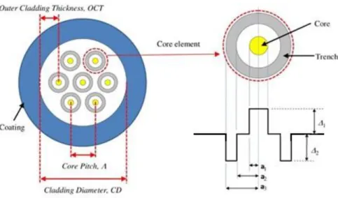
For illustration purposes, a seven core trench-assisted MCF has been chosen to represent the main parameters considered when computing the crosstalk for different proposed core arrangements (or layouts).

Three different optical fibers will be considered in this work, all sharing the same set of parameters but for the Cladding Diameter (𝐶𝑑). This parameter, often named Fiber Diameter and measuring the distance between two opposite edges of the fiber, will take a different value for each one of the three considered scenarios.

The Outer Cladding Thickness (𝑂𝐶𝑇), the distance between an Outer Core and the edge of the Outer Cladding cannot be any smaller than 30 µm, as to minimize the micro-bending loss [7]. The distance between the two ends of the optical fiber, not represented in figure 2, is defined as Fiber Length (𝐿).

The homogeneous cores placed inside the fiber, all sharing the same size and refractive indexes, will be enclosed by a trench that further confines light into the center of the core. The thickness of the trench (𝑤𝑡𝑟) and of both Cladding and Core will be the same; making the radius of the Cladding (𝑎2) and Trench (𝑎3) two and three times larger than, respectively, the radius of the Core (𝑎1). The relative refractive indexes of the Core-Cladding (∆1) and Cladding-Trench (∆2) will be identical; and by setting a cladding refractive index (𝑛2) both the core refractive index (𝑛1) and the trench refractive index (𝑛3) can be deduced.

As for the distance that separates two cores, the core pitch (Λ), it will vary in function of the different proposed layouts and number of cores integrating them. This parameter, directly correlated with XT, will be key in balancing the crosstalk values inside the fiber.

Additionally, a minimum distance of 3 µm between trench edges must be ensured as to safeguard any contact between trenches when the fiber bends [8].

Figure 2: Main parameters of a multi-core fiber

(18)

18 2.3 Crosstalk Estimation

Crosstalk, by definition, is the disturbance of a signal by the electric or magnetic field of another adjacent telecommunications signal.

Considering the way in which cores are densely packed inside a single cladding of a MCF, it shouldn’t come as a surprise that crosstalk management is crucial when dealing with coupling and the consequent degradation of transmitted signals.

Crosstalk can be described by the following expression; where 𝑃′_(𝑍)_{is the power at the output of the} reference core and 𝑃(𝑍) is the power at the output of the interfering core.

𝑋𝑇(𝑍) = 10 × 𝑙𝑜𝑔10

𝑃′(𝑍)

𝑃(𝑍)[𝑑𝐵] (2.1)

Crosstalk mitigation can be a daunting task, but if not carried out, will prevent the fiber from achieving its maximum potential in terms of performance and capacity.

For crosstalk to be properly dealt with, an accurate method for its estimation in MCFs is required. Two methods exist for doing so: Coupled-Mode Theory (CMT) and Coupled-Power Theory (CPT).

Coupled-Mode Theory (CMT), a perturbational approach for the analysis of coupling in vibrational systems, takes into account the interference between optical modes from both waveguides when these are brought sufficiently close to each other. In those cases where the electromagnetic field distributions after mode coupling don’t substantially differ from those previous to it, this method can be used to analyze the propagation characteristics of the waveguides.

While this method allows for an accurate estimation of the crosstalk while taking into account the twisting and bending effects that the fiber is subjected to, a large number of simulations are required to estimate the value of crosstalk.

Coupled-power theory, on the other hand, is based on the principle of measuring the amount of power that the signal being transmitted in one core is transferring to its neighbouring core. Unlike CMT, CPT is able to provide a fast and accurate estimation of inter-core crosstalk in MCFs by averaging the bending and twisting effects along the fiber using a predetermined correlation length 𝑑𝑐 [9].

(19)

19

MakinguseofCPT,thecrosstalkbetweentwo coreswithina fiberwithlength𝐿canbeestimatedas [10]:

𝑋𝑇 = tanh(ℎ̅𝑚𝑛𝐿) (2.2)

Moreover, if the crosstalk is very small it can be approximated as [10]:

𝑋𝑇 = ℎ̅𝑚𝑛𝐿 (2.3)

Where ℎ̅𝑚𝑛 is the average PCC between core m and core n. For the case of homogeneous fibers with a small bending radius, the average PCC can be expressed as [10]:

ℎ̅𝑚𝑛=

2𝑘𝑚𝑛2 𝑅𝑏

𝛽𝑚Λ𝑚𝑛 (2.4)

Where 𝑅𝑏 is the bending radius, Λ the core pitch and 𝛽𝑚 the propagation constant.

𝑘

𝑚𝑛, the mode coupling coefficient, is given by:

𝑘𝑚𝑛 = 𝑤𝜀0∫ ∫ (𝑁2− 𝑁𝑛2)𝐸𝑚∗ ∙ 𝐸𝑚𝑑𝑥𝑑𝑦 +∞ −∞ +∞ −∞ ∫ ∫ 𝑢𝑐 ∙ (𝐸𝑚∗ × 𝐻𝑚+ 𝐸𝑚× 𝐻𝑚∗)𝑑𝑥𝑑𝑦 +∞ −∞ +∞ −∞ (2.5)

Being 𝑤 the angular frequency of the electromagnetic field, 𝜀0 the vacuum permittivity, 𝑁2(𝑥, 𝑦) the refractive index distribution in the entire coupled region and 𝑁𝑛2 the refractive index distribution of waveguide n.

The case we’ll be considering is of a trench-assisted structure, in which three different refractive indexes can be identified: 𝑛1 for the core, 𝑛0 for the cladding and 𝑛2 for the trench. The relative refractive index difference between core and cladding is Δ1, while between trench and cladding is Δ2.

The core, cladding and trench radii relative to the center of the core are given by 𝑎1, 𝑎2 and 𝑎3 respectively; 𝑤𝑡𝑟 being the width of the trench.

Figure 3: Refractive index profile and cross-sectional dimensions of trench-assisted structure

(20)

20

For this trench-assisted case, and having under consideration that the size of the first cladding and trench are not infinitely large, the mode coupling coefficient can be estimated by the following analytical approach [10]: 𝑘′𝑚𝑛= √𝑇 ∆1 𝑎1 𝑈12 𝑉₁3_𝐾 12(𝑊1) √𝜋𝑎1 𝑊1Λ 𝑒[− 𝑊1Λ+2(𝑊2−𝑊1)𝑤𝑡𝑟 𝑎1 ] (2.6) Where 𝑈12= 𝑎12(𝑘2𝑛12− 𝛽2), 𝑊12= 𝑎12(𝛽2− 𝑘2𝑛02),𝑉1= 𝑘𝑎1𝑛1

×

√2 Δ1, 𝑊2= √𝑉22+ 𝑊12 and

𝑉2= 𝑘𝑎1

×

√𝑛02− 𝑛22. 𝑘 represents the wavenumber, λ the wavelength of light in the vacuum and 𝐾1(𝑊1) the modified Bessel function of the 2𝑛𝑑_{kind with}₁𝑠𝑡_order.

Lastly, having outlined a method to estimate the mode coupling coefficient between two cores (2.6), it is possible to estimate the crosstalk by replacing (2.4) on (2.3):

XT =2𝑘𝑚𝑛

′ 2

𝑅𝑏

𝛽Λ 𝐿 (2.7)

2.4 Crosstalk Constraints

In order to further increase transmission capacity, greater spectral efficiencies are sought by means of higher-level quadrature amplitude modulation (QAM) schemes. These modulations, along with the OSNR (Optical Signal-to-Noise Ratio) penalty they bring about, set some limitations for the maximum value of crosstalk allowed inside each core of a multi-core optical fiber.

Figure 4(c) illustrates the OSNR penalty as a function of the crosstalk. This penalty, obtained with the aid of a Monte Carlo simulation with 217 symbols, represents the SNR per symbol required to achieve a bit error rate (BER) of 10−3_{for ideal square 4-, 16-, 64- and 256-QAM constellations. Both Fig 4(a) and} Fig 4(b) show the same 16-QAM constellation (open circles) with different interferer constellations (filled circles); the first figure featuring a 16-QAM interferer constellation in-phase with the signal and the latter a 16-QAM interferer constellation with a 45º rotation relative to the signal. As expected, the case with the rotated interferer is more strongly affected due to the minimal distance between symbols, as seen in figure 4(c).

(21)

21

Three different optical fibers will be analyzed in this dissertation and for each case one must set a limit on the maximum amount of crosstalk tolerated by any core of the fiber. Two scenarios for an optical fiber link are conceived, sharing the same fiber length and differing in the chosen modulation format.

The first scenario, 1000 𝑘𝑚 in length, will feature QPSK and won’t tolerate more than 10 𝑑𝐵 of crosstalk in any of its cores (figure 4(c)). It will work with a 4 𝑑𝐵 OSNR penalty.

The second scenario, also 1000 𝑘𝑚 in length, will feature 256-QAM and won’t tolerate more than

30 𝑑𝐵 of crosstalk in any of its cores (figure 4(c)). This optical fiber link will also boast the same OSNR penalty as the previous.

Knowing that all the simulations to be presented in this dissertation were made for a fiber 100 𝑘𝑚 in length, the value of crosstalk is always expressed as 𝑑𝐵/100𝑘𝑚. Considering that the two afore mentioned scenarios express the value of crosstalk for a signal having traveled a distance of 1000 𝑘𝑚, there is the need to convert the maximum tolerable crosstalk limits from 𝑑𝐵/1000𝑘𝑚 to the 𝑑𝐵/100𝑘𝑚. Throughoutthisdissertationthecrosstalkwillbedefinedwiththenegativesign,hencethecrosstalk limits of the two previous scenarios are -10 𝑑𝐵 and -30 𝑑𝐵, for the link using QPSK and 256-QAM respectively.

By taking (2.8), a formula that relates the unitary crosstalk with the crosstalk of a signal after traveling a certain fiber length (L); then replacing the values for the two fiber lengths in question (2.9):

𝑋𝑇(𝐿) = 𝑋𝑇(1 𝑘𝑚) + 10 × log(𝐿) _(2.8)

{

𝑋𝑇

(

100

)

= 𝑋𝑇

(

1 𝑘𝑚

)

+ 10 × log (100)

𝑋𝑇

(

1000

)

= 𝑋𝑇

(

1 𝑘𝑚

)

+ 10 × log (1000) (2.9)

It is possible to determine the relation between the crosstalk of a signal that has traveled 100𝑘𝑚 and the crosstalk of that same signal after traveling 1000 𝑘𝑚:

𝑋𝑇(100) = 𝑋𝑇(1000) − 10 _(2.10)

The crosstalk tolerance of the two described optical links is therefore -20 𝑑𝐵 for the link using QPSK modulation and -40 𝑑𝐵 for the link using 256-QAM. These two different crosstalk tolerances will make up for two different designs within each one of the three different fibers to be studied in this dissertation.

Figure 4: Impact of in-band crosstalk on QAM formats; (a, b): crosstalk models; (c): Monte Carlo simulations of crosstalk penalties for ideal, square 4-, 16-, 64-, and 256-QAM [11]

(22)

22

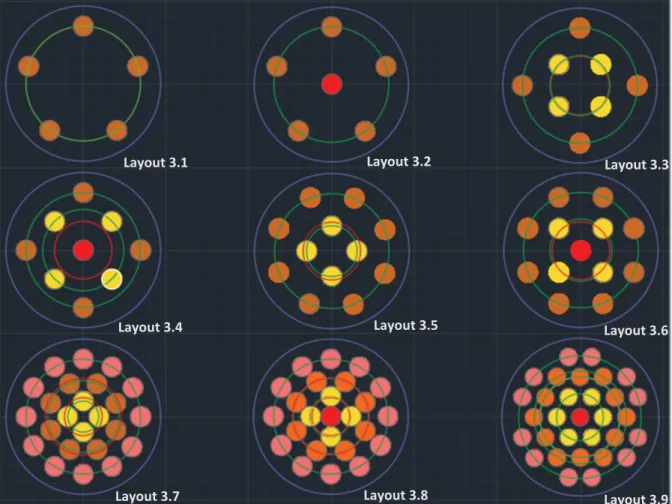
Figure 5: Proposed Layouts

3 Proposed Layouts

There are countless ways of organizing the cores inside a SM-MCF such as placing them in rings, hexagonally, or simply without any geometrical form at all. The proposed layouts will strive to balance the crosstalk across the cores, making it as low as possible for every single one in the structure. Given that three different scenarios will be studied, each with a different fiber diameter, all the proposed layouts share the possibility of enlargement (addition of cores), by making use of a precise geometry when designed. Furthermore, as the layouts needs to be commercially viable, it’s highly convenient for them to be geometrically symmetric.

Given that the crosstalk is heavily influenced by the core pitch, the logical approach for when designing the layouts would be to maximize the distance between neighbouring cores. In the light of this reasoning, circle packing theory was considered. Although circle packing theory states that the densest packing of identical circles in a plane is the hexagonal lattice of the bee’s honeycomb [12], many other geometries offer a denser packing for a specific number of circles to be packed. This being said, both these geometries and hexagonal placement will be considered. On an endnote, it is relevant to point out that unconsidered non-geometrical structures for the core allocation would sometimes produce better results for this problem of maximizing the distance between neighbouring cores.

Layout 3.1 Layout 3.1 Layout 3.4 Layout 3.4 Layout 3.8 Layout 3.8 Layout 3.7 Layout 3.7 Layout 3.6 Layout 3.6 Layout 3.2 Layout 3.2 Layout 3.3 Layout 3.3 Layout 3.9 Layout 3.8 Layout 3.5 Layout 3.6

(23)

23 3.1 One Ring

Using the One Ring layout the cores are placed evenly spaced on a circle. The radius of the circle (𝑟1), which I will name Outer Circle, is made as big as possible as to guarantee the spacing between cores is the maximum allowed by the fiber parameters. A detailed explanation on how to obtain this circle is featured in Annex A.

Initially two cores are placed in the fiber laying on the circle that

was previously described, distanced by a diameter of that same circle. More cores are then added to the fiber, one at a time, always ensuring equal spacing between a core and its neighbours until the physical limitations of the fiber prevent us from adding more cores.

Taking into consideration equation (2.7), the crosstalk calculation for each core will only take into account the interference from its two neighbours (3.1), which gives approximately the same crosstalk value as when taking all the cores into consideration. This approximation, also present in the crosstalk calculations of other Layouts, is explained in Annex B.

For the case when only have two cores incorporate the fiber (

𝑁 = 2

)

, the crosstalk calculation will be done differently as there’s only one neighbour for each core.

𝑋𝑇𝐶𝑜𝑟𝑒= 2 × 𝑋𝑇(Λ1), 𝐸𝑥𝑐𝑒𝑝𝑡 𝑓𝑜𝑟 𝑁 = 2 𝑤ℎ𝑒𝑟𝑒 𝑋𝑇𝐶𝑜𝑟𝑒= 𝑋𝑇(Λ1) (3.1)

Relevant dimensions Formula

Outer Ring radius 𝑟1

Distance between Outer Cores 𝛬1= 2𝑟1× 𝑠𝑖𝑛 (

2π

2𝑁)

Table 1: Relevant dimensions in “One Ring” Layout

(24)

24 3.2 One Ring with Central Core

One Ring with Central Core is characterized by having a set of equally spaced cores laying on the Outer Circle and a core in the center of the fiber; somewhat similar to the “One Ring” layout but with an additional core in the center.

Initially a core is placed in the center of the fiber encircled by three other cores. More cores are then added to the fiber, one by one to

the Outer Circle, always maintaining equal spacing between the cores in the Outer Circle until the physical limitations of the fiber prevent us from adding more cores.

Taking equation (2.7) and knowing the crosstalk of the cores laying on the Outer Circle will mainly come from the central core and its two neighbours, the crosstalk of an Outer Core is determined (3.3). The crosstalk calculation for the central core will take into account all the cores encircling it (3.2).

𝑋𝑇𝐶𝑒𝑛𝑡𝑟𝑎𝑙 𝐶𝑜𝑟𝑒= (𝑁 − 1) × 𝑋𝑇(𝑟1 ) (3.2)

𝑋𝑇𝑂𝑢𝑡𝑒𝑟 𝐶𝑜𝑟𝑒 = 𝑋𝑇(𝑟1) + 2 × 𝑋𝑇(Λ1) (3.3)

2π

2(𝑁 − 1))

Table 2: Relevant dimensions in “One Ring with Central Core” Layout

(25)

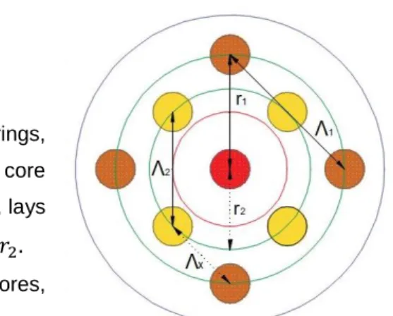
25 3.3 Two Rings

In the Two Rings layout the nuclei lay in two circumferences with different radiuses, Inner Circle and Outer Circle, each containing the same amount of nuclei. To the structure of nuclei laying on each circle I will refer as rings, with the ring boasting the larger radius (

𝑟

1) being the Outer Ring while the other, the Inner Ring, with its radius (

𝑟

2) varying in order to maintain a certain condition. When having two rings with the same number of nuclei we

expect the distance between Inner Cores (

Λ

2

)

to be smaller than the distance between Outer Cores

(Λ

1

)

, thus having the Inner Cores with the highest values of crosstalk.

In an attempt to balance the values of crosstalk, and knowing the distance between Inner Cores to be the smallest, we can move the Inner Cores further out until the distance between them is as big as the distance between two cores laying in different rings (

Λ

𝑥). The radius of the Inner Circle, containing the Inner Cores, will therefore be variable and dependent on the number of cores we decide to use in this layout. By doing this radius adjustment we are able to obtain the best possible crosstalk results for this kind of structure, as explained in Annex C.

Initially six cores are placed in the fiber, three in each ring in a way that maximizes the distance between cores in different rings. More cores are then added to the fiber, two at a time, increasing the number of cores in each ring one by one until the physical limitations of the fiber prevent us from adding more cores.

Making use of equation (2.7), it’s possible to compute the crosstalk value of an Inner Core by considering both its two neighbours and two closest Outer Cores (3.4). Similarly, when computing the crosstalk value for an Outer Core, only its two neighbours and two closest Inner Cores are taken into consideration (3.5).

𝑋𝑇𝐼𝑛𝑛𝑒𝑟 𝐶𝑜𝑟𝑒= 2 × 𝑋𝑇(Λ2) + 2 × 𝑋𝑇(Λ𝑥) (3.4)

𝑋𝑇𝑂𝑢𝑡𝑒𝑟 𝐶𝑜𝑟𝑒 = 2 × 𝑋𝑇(Λ1) + 2 × 𝑋𝑇(Λ𝑥) (3.5)

2π

2𝑀1)

Inner Ring radius _𝑟

2= (2𝑟1×𝑐𝑜𝑠(_2𝑀12π))−√(−2𝑟1×𝑐𝑜𝑠(_2𝑀12π)) 2 −4×(1−4𝑠𝑖𝑛2(2π 2𝑀1))×(𝑟12) 2×(1−4𝑠𝑖𝑛2₍2π 2𝑀1))

Distance between Inner Cores 𝛬2= 2𝑟2× 𝑠𝑖𝑛 (

2π

2𝑀2)

Inner-Outer Core distance 𝛬𝑥= 𝛬2

Table 3: Relevant dimensions in “Two Rings” Layout

(26)

26 3.4 Two Rings with Central Core

Two Rings with Central Core distributes its cores in two rings, each containing the same number of cores, with an additional core present in the center. The Outer Ring, with the larger radius, lays at a distance

𝑟

1 from the center while the Inner Ring ranges

𝑟

2

.

The Inner Ring radius will be dependent on the number of cores, always bigger than half the Outer Ring radius, varying to ensure the distance from an Inner to the Central core remains the same

as the distance from an Inner to the closest Outer Core. By doing this we expect to better balance the values of crosstalk when comparing to a similar structure in which the Inner Cores would be placed at half the Outer Ring radius. This procedure is explained in Annex D.

Initially seven cores are placed in the fiber, three in each ring in a way that maximizes the distance between cores in different rings, plus another core in the center. More cores are then added to the fiber, two at a time, increasing the number of cores in each ring one by one until the physical limitations of the fiber prevent us from adding more cores.

From equation (2.7), we compute the crosstalk value of an Inner Core by considering its two neighbours, two closest Outer Cores and the central core (3.7). Similarly, when computing the crosstalk of an Outer Core we only take into account its two neighbours, closest Inner Core and the Central Core (3.8). The crosstalk calculation for the central core will take into account all the cores encircling it (3.6).

𝑋𝑇𝐶𝑒𝑛𝑡𝑟𝑎𝑙 𝐶𝑜𝑟𝑒= 𝑀1× 𝑋𝑇(𝑟1) + 𝑀2× 𝑋𝑇(𝑟2) (3.6)

𝑋𝑇𝐼𝑛𝑛𝑒𝑟 𝐶𝑜𝑟𝑒 = 𝑋𝑇(𝑟2) + 2 × 𝑋𝑇(Λ2) + 2 × 𝑋𝑇(Λ𝑥) (3.7)

𝑋𝑇𝑂𝑢𝑡𝑒𝑟 𝐶𝑜𝑟𝑒 = 𝑋𝑇(𝑟1 ) + 2 × 𝑋𝑇(Λ1) + 2 × 𝑋𝑇(Λ𝑥) (3.8)

2π

2𝑀₁)

Inner Ring radius 𝑟2=

𝑟1 2 𝑐𝑜𝑠(2π

2𝑀1)

2π

2𝑀2)

Inner-Outer Core distance 𝛬𝑥 = 𝑟2

Table 4: Relevant dimensions in “Two Rings with Central Core” Layout

(27)

27 3.5 Two Different Rings

Two Different Rings organizes its cores in two rings, where the Inner Ring has half the number of cores than the Outer Ring. This new approach to the two ring layout comes as an attempt to more evenly balance the distance between neighbouring cores in both rings, in which the Outer Ring is placed at a distance

𝑟

1 from the center and the Inner Ring at a distance

𝑟

2.

Similarly to the “Two Ring” layout, the Inner Core Crosstalk is the

limiting factor in this layout. In order to minimize the Inner Core Crosstalk, we adjust the Inner Ring radius as to ensure that the distance between Inner Ring neighbours (

Λ

2) is the same as the distance between an Inner Core and the closest Outer Cores (

Λ

𝑥); in other words, we guarantee that an Inner Core is equally spaced to its closest neighbour and Outer Core. This procedure is explained in Annex E.

Initially nine cores are placed in the fiber, six in the Outer plus three in the Inner Ring in a way that maximizes the distance between cores in different rings. More cores are then added to the fiber, three at a time, increasing respectively by one and two at a time the number of cores in the Inner and Outer Ring until the physical limitations of the fiber prevent us from adding more cores.

Making use of equation (2.7), it’s possible to compute the crosstalk value of an Inner Core by considering its two neighbours and two closest Outer Cores (3.9). When computing the crosstalk of an Outer Core, its two neighbours and closest Inner Core are considered (3.10).

𝑋𝑇𝐼𝑛𝑛𝑒𝑟 𝐶𝑜𝑟𝑒 = 2 × 𝑋𝑇(Λ2) + 2 × 𝑋𝑇(Λ𝑥) (3.9)

𝑋𝑇𝑂𝑢𝑡𝑒𝑟 𝐶𝑜𝑟𝑒 = 2 × 𝑋𝑇(Λ1) + 𝑋𝑇(Λ𝑥) (3.10)

2π

2𝑀1)

Inner Ring radius _𝑟

2= (2𝑟1×𝑐𝑜𝑠(_2𝑀12π))−√(−2𝑟1×𝑐𝑜𝑠(_2𝑀12π)) 2 −4(1−4𝑠𝑖𝑛2₍2π 2𝑀2))×(𝑟12) 2×(1−4𝑠𝑖𝑛2₍2π 2𝑀2))

2π

2𝑀2)

Inner-Outer Core distance 𝛬𝑥= 𝛬2

Table 5: Relevant dimensions in “Two Different Rings” Layout

(28)

28 3.6 Two Different Rings with

Central Core

Two Rings with Central Core organizes its cores in two rings plus another core in the center, where the Inner Ring has half the cores the Outer Ring has. The Outer Ring, with the larger radius, laying at a distance

r

1 and the Inner Ring at a distance

r

2 from the center.

The Inner Ring radius will be dependent on the number of cores, always bigger than half the Outer Ring radius, varying to ensure the distance from an Inner to the Central core remains the same as the distance from an Inner to the closest Outer Cores. By doing so we expect to better balance the values of Crosstalk when comparing to a similar structure in which the Inner Cores would be placed at half the Outer Ring radius. This procedure is explained in Annex F.

Initially seven cores are placed in the fiber, one in the center, four in the Outer and two in the Inner Ring in a way that maximizes the distance between cores in different rings. More cores are then added to the fiber, three at a time, increasing respectively by one and two at a time the number of cores in the Inner and Outer Ring until the physical limitations of the fiber prevent us from adding more cores.

Taking equation (2.7) into account, it’s possible to compute the crosstalk value of an Inner Core by taking into consideration its two neighbours, two closest Outer Cores and the Central core (3.12). Similarly, when computing the crosstalk value for an Outer Core only its two neighbours, closest Inner Core and central core are considered (3.13). The crosstalk calculation for the central core will take into account all the cores encircling it (3.11).

𝑋𝑇𝐶𝑒𝑛𝑡𝑟𝑎𝑙 𝐶𝑜𝑟𝑒= 𝑀1× 𝑋𝑇(𝑟1 ) + 𝑀2× 𝑋𝑇(𝑟2) (3.11)

𝑋𝑇𝐼𝑛𝑛𝑒𝑟 𝐶𝑜𝑟𝑒= 𝑋𝑇(𝑟2) + 2 × 𝑋𝑇(Λ2) + 2 × 𝑋𝑇(Λ𝑥) (3.12)

𝑋𝑇𝑂𝑢𝑡𝑒𝑟 𝐶𝑜𝑟𝑒= 𝑋𝑇(𝑟1 ) + 2 × 𝑋𝑇(Λ1) + 𝑋𝑇(Λ𝑥) (3.13)

2π

2𝑀1)

Inner Ring radius 𝑟2=

𝑟1 2 𝑐𝑜𝑠(2π

2𝑀1)

2π

2𝑀₂)

Inner-Outer Core distance 𝛬𝑥= 𝑟2

Table 6: Relevant dimensions in “Two Different Rings with Central Core” Layout

(29)

29 3.7 Three Different Rings

Three Different Rings has its cores organized in three rings, where both the Inner and Middle Rings have, respectively, a third and two thirds of the cores composing Outer Ring. The Outer Ring, boasting the largest radius, lays at a distance

r

1 from the center while the Inner Ring at a distance

r

3 from the center. The ring that lays in-between these two goes by Middle Ring, and lays at a distance

r

2

from the center of the layout.

Both the Middle and Inner Ring radii will be dependent on the number of cores, changing in order to maintain the distance between Inner Ring neighbours the same as both the distance between an Inner Core and its closest Middle Core and between a Middle Core and the Outer Circle.

It is important to note that the distance between an Outer Core and its closest Middle Core will depend on the Outer Core we pick, which is why it is necessary to make the distance between Inner Ring neighbours the same as the distance between a Middle Core and the Outer Circle, to ensure this latter is either the same or smaller than the distance between a Middle and an Outer Core. This algorithm produces better crosstalk results when comparing to a similar structure where the rings are equally spaced, as explained in Annex G.

Initially eighteen cores are placed in the fiber, nine in the Outer Ring, six in the Middle Ring and three in the Inner Ring in a way that maximizes the distance between cores in different rings. More cores are then added to the fiber, six at a time, increasing respectively by one, two and three at a time the number of cores in the Inner, Middle, and Outer Ring until the physical limitations of the fiber prevent us from adding more cores.

From equation (2.7), we can compute the crosstalk of an Inner Core by taking into account both its neighbours and two closest Middle Cores (3.14). For the crosstalk of a Middle Core, its two neighbours are considered as well as its closest Inner and Outer Core (3.15). As for the crosstalk of an Outer Core, its two neighbours and closest Middle Core are taken into account (3.16).

It is important to note that due to the variable distance between different Middle Cores and their closest Outer Cores, when I refer to that distance I’m actually considering the distance between a Middle Core and the Outer Circle, thus always guaranteeing the former distance to be equal or greater than the one considered.

𝑋𝑇𝐼𝑛𝑛𝑒𝑟 𝐶𝑜𝑟𝑒= 2 × 𝑋𝑇(Λ3) + 2 × 𝑋𝑇(Λ𝑥) (3.14)

𝑋𝑇𝑀𝑖𝑑𝑑𝑙𝑒 𝐶𝑜𝑟𝑒 = 𝑋𝑇(Λ𝑥) + 𝑋𝑇(Λ𝑥) + 2 × 𝑋𝑇(Λ2) (3.15)

(30)

30

Relevant dimensions Formula Outer Ring radius 𝑟1 Distance between Outer Cores 𝛬1= 2𝑟1× 𝑠𝑖𝑛 ( 2π 2𝑀1 ) Inner Ring radius 𝑟3= 2𝑟1×𝑐𝑜𝑠(_2𝑀22π)+4𝑟1×𝑠𝑒𝑛(_2𝑀32π)−√(−2𝑟1×𝑐𝑜𝑠(_2𝑀22π)−4𝑟1×𝑠𝑒𝑛(_2𝑀32π)) 2 −4×(1+4 𝑠𝑖𝑛(2π 2𝑀3) 𝑐𝑜𝑠( 2π 2𝑀2))×(𝑟12) 2×(1+4 𝑠𝑖𝑛(2π 2𝑀3) 𝑐𝑜𝑠( 2π 2𝑀2)) Distance between Inner Cores 𝛬3= 2𝑟3× 𝑠𝑖𝑛 ( 2π 2𝑀3 ) Middle Ring radius 𝑟2= 𝑟1− 𝛬3 Distance between Middle Cores 𝛬2= 2𝑟2× 𝑠𝑖𝑛 ( 2π 2𝑀2 ) Inner-Middle-Outer Core distance 𝛬𝑥 = 𝛬3

Table 7: Relevant dimensions in “Three Different Rings” Layout

3.8 Three Different rings with Central

Core

Three Different Rings with Central Core is a layout in which the nuclei are organized in three rings and a central core, where both the Inner and Middle Rings have, respectively, a third and two thirds of the cores composing the Outer Ring. The Outer Ring, boasting the largest radius, lays at a distance

𝑟

1 from the center

while the Middle and Inner Ring at a distance of, respectively,

𝑟

2and

𝑟

3from the center.

Both the Middle and Inner Ring radii will be dependent on the number of cores, varying in order to maintain constant the distance from the Central Core to an Inner Core, from an Inner Core to a Middle Core and from a Middle Core to the Outer Circle. It is important to note that the distance between an

(31)

31

Outer Core and its closest Middle Core will depend on the Outer Core we pick, which is why it is necessary to make the distance from the Central Core to an Inner Core the same as the distance between a Middle Core and the Outer Circle, to ensure this latter is either the same or smaller than the distance between a Middle and an Outer Core. This algorithm produces better crosstalk results when comparing to a similar structure in which the rings are equally spaced, as explained in Annex H.

Initially nineteen cores are placed in the fiber, one in the center, nine in the Outer Ring, six in the Middle Ring and three in the Inner Ring in a way that maximizes the distance between cores in different rings. More cores are then added to the fiber, six at a time, increasing respectively by one, two and three at a time the number of cores in the Inner, Middle, and Outer Ring until the physical limitations of the fiber prevent us from adding more cores.

Making use of equation (2.7), it’s possible to determine the crosstalk of an Inner Core taking under consideration its two neighbours, two closest Middle Cores and the central core (3.18). For the crosstalk of a Middle Core, its two neighbours are considered as well as its closest Inner and Outer Cores (3.19). As for the crosstalk of an Outer Core, its two neighbours and closest Middle Core are taken into account (3.20). The crosstalk calculation for the central core will take into account all the cores encircling it (3.17). It is important to note that due to the variable distance between different Middle Cores and their closest Outer Cores, when I refer to that distance I’m actually considering the distance between a Middle Core and the Outer Circle, thus always guaranteeing the former distance to be equal or greater than the one considered.

𝑋𝑇𝐶𝑒𝑛𝑡𝑟𝑎𝑙 𝐶𝑜𝑟𝑒 = 𝑀1× 𝑋𝑇(𝑟1 ) + 𝑀2× 𝑋𝑇(𝑟2) + 𝑀3× 𝑋𝑇(𝑟3 ) (3.17)

𝑋𝑇𝐼𝑛𝑛𝑒𝑟 𝐶𝑜𝑟𝑒 = 𝑋𝑇(𝑟3 ) + 2 × 𝑋𝑇(Λ3) + 2 × 𝑋𝑇(Λ𝑥) (3.18)

𝑋𝑇𝑀𝑖𝑑𝑑𝑙𝑒 𝐶𝑜𝑟𝑒= 𝑋𝑇(Λ𝑥) + 𝑋𝑇(Λ𝑥) + 2 × 𝑋𝑇(Λ2) (3.19)

2π

2𝑀1)

Middle Ring radius 𝑟2=

𝑟1 1+2𝑐𝑜𝑠 (2π

2𝑀2)

Distance between Middle Cores 𝛬2= 2𝑟2× 𝑠𝑖𝑛 (

2π

2𝑀2)

Inner Ring radius 𝑟3= 𝑟1− 𝑟2

2𝜋 2𝑀₃) Inner-Middle-Outer Core

distance 𝛬𝑥 = 𝑟3

(32)

32 3.9 Hexagonal Placement

With Hexagonal Placement the cores are organized in different rings, all having a hexagonal shape. Different nuclei in the same ring can have different distances to the center, meaning that rings are not, unlike in previous layouts, characterized by having all its nuclei equidistant to the center. There’s always a ways a central core present in this layout and the inter-core distance between any two adjacent cores is constant.

The way in which we add cores to this layout is more complex than one might think. Rings cannot be simply added to the fiber until the physical limitations of the fiber allow, since some cores in the same ring may differ in distance to the central core; meaning some cores may fit inside the fiber while others don’t. For this reason, whenever cores are added to the fiber they all share the same radius; meaning rings are built in one, two, three and sometimes more phases.

Initially seven cores are placed in the fiber, as all the six cores composing the first ring have the same radius 𝑅1. We then construct part of the second ring by adding those cores that are closest to the center (𝑅21) before being able to complete it by adding the remaining cores at a distance 𝑅22 from the center. Having the second ring in place, built in two iterations, we persist adding more cores a few at a time crafting only part each rings on each iteration until we can no longer fit any more cores in the fiber. The colored hexagons in figure 15, in which the cores will be inscribed, mark the different iterations.

Core pitch 𝛬 1𝑠𝑡_{𝑅𝑖𝑛𝑔 − 𝐺𝑟𝑒𝑒𝑛} _𝑅 1= 𝛬 2𝑛𝑑_{𝑅𝑖𝑛𝑔(1) – 𝐵𝑙𝑢𝑒} _𝑅 21= 2𝛬 × 𝑐𝑜𝑠 (30) 2𝑛𝑑_{𝑅𝑖𝑛𝑔(2) – 𝑅𝑒𝑑} _𝑅₂₂_{= 2𝛬} 3𝑟𝑑_{𝑅𝑖𝑛𝑔(1) − 𝐶𝑦𝑎𝑛} _𝑅 31= √7𝛬 3𝑟𝑑_{𝑅𝑖𝑛𝑔(2) − 𝑌𝑒𝑙𝑙𝑜𝑤} _𝑅 32= 3𝛬 4𝑡ℎ_{𝑅𝑖𝑛𝑔(1) − 𝑂𝑟𝑎𝑛𝑔𝑒} _𝑅 41= 4𝛬 × 𝑐𝑜𝑠 (30) 4𝑡ℎ𝑅𝑖𝑛𝑔(2) − 𝑃𝑖𝑛𝑘 𝑅42= √13𝛬 4𝑡ℎ_{𝑅𝑖𝑛𝑔(3) − 𝐿𝑖𝑔ℎ𝑡 𝐺𝑟𝑒𝑒𝑛} _𝑅 43= 4𝛬

Table 9: Relevant dimensions in "Hexagonal Placement” Layout

Given that the inter-core distance is the same between any two adjacent cores in the structure, for the crosstalk calculation we only need to multiply the value of crosstalk between any two cores with the number of adjacent cores to it:

𝑋𝑇𝐺𝑖𝑣𝑒𝑛 𝐶𝑜𝑟𝑒= 𝑁º𝐴𝑑𝑗𝑎𝑐𝑒𝑛𝑡 𝐶𝑜𝑟𝑒𝑠 × 𝑋𝑇(𝛬) (3.21)

Figure 14: Hexagonal Placement

Figure 15: Different iterations in “Hexagonal Placement” construction process

(33)

33 4 Implementation

4.1 Numerical Model

A MatLab algorithm was used to determine and plot, for each proposed layout, the different crosstalk values as a function of the number of cores featured in it.

Figure 16 describes the use of this algorithm for the first theoretical model, the “One Ring” layout. In this model, the initial number of cores is two and the way to add more cores is one at a time.

(34)

34 4.2-Verification and Validation

Having developed an algorithm to predict the crosstalk in each core of a given layout, it is necessary to ensure the results it produces are in accordance with the results from other related papers. For doing so, a comparison with a 2014 paper [8] on homogeneous TA-MCF was made.

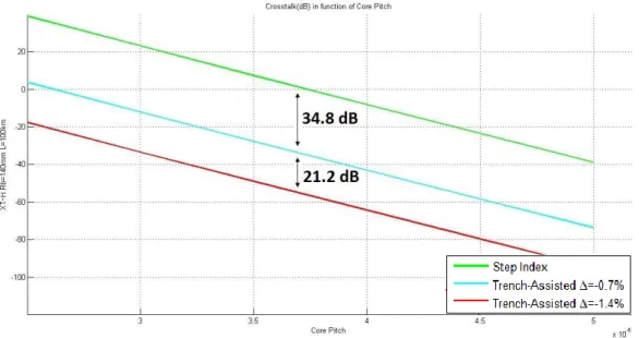
Plots of the crosstalk as a function of the core pitch were extracted from this paper; figure 17.

Three lines can be seen in figure 17; a dotted blue one for the step-index profile and two purple ones for the assisted profile, which requires a slightly different calculation method. For the trench-assisted profile two cases with different relative refractive indexes are presented; one with ∆2= −0.7% and another with ∆2= −1.4% having 21 𝑑𝐵 less crosstalk.

It becomes clear that the use of a trench drastically reduces the inter-core crosstalk. As the relative refractive index of the cladding-trench increases, the more confined light becomes in the cores and the less inter-core crosstalk is verified.

As for the crosstalk computing algorithm previously presented in this dissertation, its results are depicted in figure 18:

(35)

35

Both simulations yield nearly identical results, with the gaps between plots differing less than 1 𝑑𝐵. Having proven the validity and accuracy of the proposed crosstalk calculation algorithm, it is safe to proceed and make use of it to analyze the crosstalk behavior of the proposed layouts.

(36)

36 5 Results

5.1 Problem Description

Single-mode optical fiber transmission systems are rapidly approaching its fundamental limit, reaching capacities up to roughly 100Tb/s per fiber [13] by employing various state-of-the-art multiplexing techniques (figure 19).

In order to overcome the impending capacity crunch we turn to space-division multiplexing, more precisely single-mode multi-core optical fibers, as a solution to overcome these capacity limits.

Fibers containing multiple cores with reasonable values of

crosstalk will achieve larger capacities than those with only one. This being said, a method to spatially set up the cores and minimize their crosstalk is sought.

In accordance with the fiber parameters mentioned in table 10, several layouts were proposed and their crosstalk results generated by means of a MatLab simulation. An analysis of these results will now help determine the number of cores that should be placed inside the fiber to maximize its capacity.

Three different scenarios will be considered and analyzed. One in which the cladding diameter is 260 µ𝑚, another in which it is 300 µ𝑚 and one last in which it is 125 µ𝑚.

Parameter Unit Value

𝐶𝑑 [µ𝑚] 125, 260, 300 𝑂𝐶𝑇 [µ𝑚] 30 𝐿 [𝑘𝑚] 100 𝑎1 [µ𝑚] 4.5 𝑎3/𝑎1 -- 3 𝑎2/𝑎1 -- 2 𝑤𝑡𝑟/𝑎1 -- 1 𝑛1 -- 1.4551 ∆1 % 0.35 ∆2 % 0.35 λ [𝑛𝑚] 1550 𝑅𝑏 [𝑚𝑚] 140

Table 10: Structural Parameters of the considered TA-MCF

(37)

37 5.2 Baseline Solution

When trying to maximize the number of cores inside a fiber, several are the possible layouts. This section will focus on a particular one [14], published on the 16th of May 2016, that makes use of an hexagonal structure to distribute thirty-one homogeneous trench-assisted cores inside a 230 µ𝑚 fiber (figure 20).

This layout, presenting a high core-count homogeneous MCF solution, was employed on a fiber with different parameters from those used in this dissertation’s simulations. In order to allow for a fair comparison to be made between this layout and those previously proposed in this dissertation, a new simulation is required.

Considering the same fiber parameters as those used in all simulations throughout this dissertation (Table 10) and choosing 260 µ𝑚 as the cladding diameter, it is possible to obtain the crosstalk values of each core in the layout (figure 21).

Despite the appearance, figure 21 show this layout has a very balanced distribution amongst the cores, which is a very good indicator that it is suited for the placement of this many cores in a fiber.

Given that the distance between any two given cores in the layout is constant, the amount of crosstalk present on each will be proportional to the number of adjacent cores. Having said so, it is now clear that the cores in layer four have the smallest value of crosstalk, followed by those in layer three that only have five neighbours. The remaining cores, in layers one, two and three, share the highest value of crosstalk as all of them are surrounded by six cores.

Figure 20: (a): A fabricated homogeneous 31-core fiber; (b): The definition of layer and core numbers [14]

Figure 21: Crosstalk of different layers – 31 Core Hexagonal layout from [14]

(38)

38 5.3 Enhanced Solution

Providing an optimal solution for the problem of core allocation in MCF’s is an elusive task. Many layouts were proposed for the core distribution inside the fiber but only after a thorough study of the crosstalk behavior in each is it possible to conclude which should be chosen.

Three different cases will be studied separately, each featuring an optical fiber with a well-defined set of parameters. Cladding diameter, the only parameter varying between cases, will be 260 µ𝑚 in the first one for it’s the highest value manufacturers are currently able to achieve.

The proposed layouts will then be used to spatially distribute the cores in the fiber, and with the help of MatLab, their crosstalk results compared.

After having figured out what the best layout is for the first case, two more will be studied. One case featuring a fiber 300 µ𝑚 in cladding diameter, as deemed feasible in a near future, and another 125 µ𝑚

much like most single mode fibers employed nowadays.

5.3.1 First Case:

𝑪𝑫 = 𝟐𝟔𝟎 𝝁𝒎

In order to determine which layout suits best for a given number of cores, it is necessary to analyze the behavior of crosstalk as a function of the number of cores for all the proposed layouts. In the following analysis the filled circles represent the values of crosstalk for a given number of cores whereas the solid lines illustrates the trend described by a given set of crosstalk values.

One Ring

The crosstalk of a core, expressed in 𝑑𝐵, increases as more and more cores integrate the structure, being inversely proportional to the inter-core distance. We can see that when placing the cores this way no more than twenty cores can fit inside the fiber.

Study and optimization of core allocation in multi-core optical fibers

1