Document downloaded from:
This paper must be cited as:
The final publication is available at
Copyright
Additional Information
http://hdl.handle.net/10251/135018
Llorca Garcia, C.; Moreno, AT.; García García, A. (2016). Modelling vehicles acceleration
during overtaking manoeuvres. IET Intelligent Transport Systems. 10(3):206-215.
https://doi.org/10.1049/iet-its.2015.0035
https://doi.org/10.1049/iet-its.2015.0035
Modelling vehicles acceleration
1
during overtaking manoeuvres
2 3 Carlos Llorca 4 PhD, Research assistant 5
Highway Engineering Research Group 6
Universitat Politècnica de València 7
Camino de Vera s/n 46022, Valencia (Spain) 8 +34 96 3877374 9 [email protected] 10 11
Ana Tsui Moreno 12
PhD, Research assistant Highway Engineering Research Group 13
Universitat Politècnica de València 14 [email protected] 15 16 Alfredo Garcia 17 Professor 18
Highway Engineering Research Group 19
Universitat Politècnica de València 20
21 22
Keywords: two-lane rural road, overtaking sight distance, assistance system, microsimulation 23
Abstract
24
Overtaking manoeuvre is a key issue for two-lane rural roads. These roads should provide suffi-25
cient overtaking sight distance at certain locations to allow faster vehicles to pass slower ones. 26
However, overtaking requires occupying the opposing lane, which represents a serious safety 27
concern. Severity of overtaking related crashes is very high, compared to other manoeuvres. The 28
development of Advanced Driver Assistance Systems (ADAS) for overtaking is being a complex 29
task. Only few systems have been developed, but are not still in use. This research incorporated 30
accurate data of real manoeuvres to improve the knowledge of the phenomenon. The trajectory 31
of the overtaking vehicles on the left lane was observed. An instrumented vehicle measured the 32
overtaking time and distance, the abreast position, and the initial and final speed of 180 drivers 33
that passed it during a field experiment. Six different kinematic models (such as uniform acceler-34
ation or linear variation of acceleration) were calibrated. Generally, drivers started to accelerate 35
before changing to the opposing lane. These models may be applied to ADAS, to estimate over-36
taking sight distance and to improve microsimulation models. 37
1. Introduction and background
38
On two-lane rural roads, vehicles travelling at slower speeds cause delays to faster vehicles. 39
Overtaking manoeuvres allow faster drivers to travel at their own desired speed, hence minimizing 40
these delays. However, any overtaking manoeuvre requires to occupy the opposing lane to pass 41
a slower vehicle. Therefore, the risk of collision with the opposing traffic affects both operation 42
and safety. 43
The severity of accidents related to overtaking manoeuvres is usually higher than in other ma-44
noeuvres [1]. To complete an overtaking manoeuvre, the overtaking vehicle must increase its 45
speed in order to pass a slower vehicle and return to the right lane. At the same time, an opposing 46
vehicle could be approaching at a relatively high speed. The potential collision risk during the time 47
the left lane is occupied makes driving behaviour different from other conditions, such as free-48
flow or following situations. To ensure road safety, overtaking is only allowed in the zones where 49
available sight distance is higher than the required Overtaking Sight Distance (OSD). OSD is 50
defined as the distance required to complete an overtaking manoeuvre when an opposing vehicle 51
is approaching. OSD has been traditionally estimated using different overtaking manoeuvre mod-52
els. The assumptions of those models, especially in relation to the overtaking vehicle acceleration 53
and its variation, vary significantly and are not verified with field data. The knowledge of the values 54
of the acceleration of the overtaking vehicle, as well as they possible variation during the ma-55
noeuvre, is one of the key issues in determining OSD. 56
Drivers make overtaking decisions according to their own behaviour and experience, as well as 57
to road and traffic perception. According to Gray et al. [2], decisions during overtaking are based 58
on drivers’ perception of distance and time to collision with the oncoming traffic. They conclude 59
that drivers tend to make more errors when their decisions are based only on the distance, after 60
a driving simulator experiment with only 18 drivers. However, the estimation of the speed of op-61
posing vehicles is extremely difficult, because of the very low rate of expansion of objects located 62
so far from the observer. Additionally, Basilio et al. [3] and Morice et al. [4] proposed an overtaking 63
decision model based on the overtaking ability affordance, defined as the quotient between the 64
minimum speed required to overtake and the maximum speed of the vehicle at that time, depend-65
ing on the vehicle performance. After a driving simulator experiment with only 16 drivers, they 66
evidenced that drivers accurately perceived whether a lead vehicle can be safely overtaken, since 67
overtaking attempt decreased with the real possibility to overtake. Alternatively, Farah et al. [5] 68
modelled risk during overtaking maneuvers, by predicting Time To Collision (TTC) based on a 69
driving simulator experiment with up to 100 drivers. 70
Driving simulator experiments confirmed the fact that overtaking manoeuvre is one of the most 71
difficult ones. The use of driving simulator might limit the validity of findings, as risk taken by 72
drivers depends on their immersion in the virtual world during the experiment, and the detection 73
of opposing vehicles which at long distances is complicated, due to the limited resolution of 74
screens. Besides, driving simulator usually only accounts for a very limited (or null) variability of 75
acceleration capabilities of vehicles, because only one type [3] or two types [4] of vehicle are 76
implemented. Consequently, a field study is solely able to study drivers’ behaviour across a wide 77
range of vehicles in real conditions. 78
79
1.1. Overtaking models
80
In some cases, speed of overtaking vehicle was assumed to be uniform during the left lane occu-81
pation time [6], although an acceleration stage was identified before occupying the left lane. This 82
uniform speed model proposed an average acceleration rate of 0.62 m/s2. Other models have
83
used more complex kinematic equations, in order to describe overtaking vehicle trajectories [7]– 84
[10]. Those usually suggested the existence of a critical point. After the critical point, it is safer to 85
complete the overtaking manoeuvre rather than to abort it, because the time and distance re-86
quirements for this are lower. According to these models, the overtaking vehicle accelerates at a 87
constant rate until the critical position and after that position; speed is constant and equal to the 88
design speed. Alternative formulations were: uniform acceleration models [11] uniform accelera-89
tion until a target speed [12], or models based on a variable acceleration that decreased linearly 90
as speed increased [13]. 91
On the other hand, some authors accounted uncertainty in the overtaking process using reliability 92
analysis or simulation techniques. These statistical tools could account the variability of input 93
parameters and provide a probabilistic formulation for overtaking sight distance. Sparks et al. [14] 94
used Glennon’s and Liebermann’s models incorporating statistical distributions of input parame-95
ters. Hanley and Forkenbrok [15] performed a simulation with previous OSD models, incorporat-96
ing random distributions of input parameters, too. El Khoury and Hoberika [16] proposed a Monte 97
Carlo simulation to evaluate risk level of OSD Glennon’s model. The statistical distributions of 98
acceleration rates were obtained from previous research works, although they were not related 99
to overtaking manoeuvre studies. El Bassiouni and Sayed [17] developed a reliability analysis to 100
compare AASHTO OSD model [6] with driving simulator data. However, the assumptions of that 101
model remained unverified. 102
Other studies have used data of driving simulator experiments to analyse the acceleration of 103
overtaking vehicles. Jenkins and Rilett [18] characterized the distribution of time spent accelerat-104
ing for a sample of 96 manoeuvres. It was observed that on average the acceleration time was 105
13.3 s, being the average overtaking time up to 20,0 s, clearly double as most of field data, ac-106
cording to the authors. Besides, the acceleration capabilities of the simulated vehicles were uni-107
form for all drivers. Rakha et al. [19] collected data of acceleration rates of different passenger 108
cars performing an experiment under controlled conditions. The relationships between accelera-109
tion rates and speed were determined. The experiment was based on an acceleration movement 110
starting at 0 km/h. Therefore, this results cannot be directly applied to overtaking manoeuvres, 111
since acceleration rates can be different depending on the speed the manoeuvre starts and on 112
driver reaction to a potential risky situation. 113
Some field studies [20], [21] recorded overtaking manoeuvres in order to calibrate the 2001 114
AASTHO model parameters using experimental data. However, they frequently did not verify as-115
sumptions of those models either (such as the fact that acceleration was uniform until reaching 116
the design speed). Others authors [22], [23] have used instrumented vehicles to analyse the over-117
taking process on two-lane rural roads. Carlson et al. [22] described the evolution of overtaking 118
vehicle speed, showing an initial acceleration stage followed by a second stage (after the abreast 119
position) where acceleration was lower. However, Carlson et al. did not try to calibrate any accel-120
eration model, and the distances to the overtaking vehicle were obtained from video data. Be-121
sides, they did not measure instant speed values at the start and the beginning of the manoeuvre. 122
1.2. Assistance systems
123
A further step after the prediction of the required OSD is the development of Advanced Driver 124
Assistance Systems (ADAS). The benefits for ADAS may improve drivers’ judgement errors, but 125
they are not as common in overtaking as in other manoeuvres, such as lane changing or car-126
following. In fact, there are only few prototypes without real implementation. 127
As expressed by Morice et al. [4], ADAS for overtaking should be calibrated to be effective. It 128
means that they should be coherent with drivers’ behaviour. Therefore, individuals would agree 129
with the system. 130
The effectiveness of ADAS has been already tested using microsimulation model RuTSim [24]. 131
Those authors analysed safety benefits of an assistance system to warn drivers that were accept-132
ing an opposing gap too small. Either the effect on road safety (measured by the Time to Collision 133
– TTC - with the opposing vehicle) or the effect on traffic operation (Average Travel Speed – ATS 134
- and delay) were limited. In absence of accurate data of overtaking manoeuvres, the authors 135
used several thresholds for TTC (equal to left lane occupation time plus a safety margin) ranging 136
from 8 to 14 s. One of the main shortcomings of the proposed system is that the overtaking 137
threshold were pre-programmed and do not depend on the current conditions. 138
A different study conducted by Milanés et al. focused on the experimental simulation of assistance 139
systems under controlled conditions [25]. The system depended on stereo vision to detect the 140
preceding vehicle and to activate the automated overtaking system. Longitudinal and lateral con-141
trollers were tested in an experiment where the impeding vehicle was travelling at very low speed. 142
The presence of opposing traffic was not considered. 143
Isermann et al. [26] proposed an assistance system to warn driver of dangerous overtaking ma-144
noeuvres, because of the presence of opposing vehicles. The system would detect opposing 145
vehicles when an overtaking manoeuvre has been initiated. Dangerous situations would result in 146
a warning signal (to encourage the driver to abort) or even in an emergency braking. Both over-147
taking model and safety margins were not calibrated, though. Petrov and Nashashibi [27] devel-148
oped a mathematical model and an adaptive controller for automated overtaking. The system was 149
tested using driving simulation, but it has not been compared with real data. 150
Lastly, Lowenau et al. [28] developed a overtaking assistance system based on the characteriza-151
tion of the previous driving behaviour (speed, acceleration, etc.) and geographical information 152
provided by a GPS tracker. This system would encourage or discourage drivers to pass depend-153
ing on the road and on their behaviour. However, this system does not provide information on the 154
opposing traffic presence. 155
As can be seen, most of the previous studies propose potential solutions to develop ADAS for 156
overtaking. Most of them were based only on numerical simulations [24], [26], or driving simulator 157
studies [27] and were not programmed after observing the real behaviour. Driving data in real 158
conditions is still needed to produce ADAS on the conditions that drivers may encounter in the 159
real world. Those systems that can avoid drivers’ errors require determining the thresholds for 160
safe overtaking, in terms of distance travelled on the left lane and subsequently, acceleration 161
rates. In absence of an accurate estimation of this variable, it is not possible to take into account 162
the real risk of collision with opposing traffic. 163
1.3. Research motivation
164
The effects of overtaking manoeuvre on road safety and road operation motivate the improvement 165
of design and marking of two-lane rural roads and the development of ADAS. With this purpose, 166
the estimation of the duration and distance of occupation of the opposing lane is needed. The 167
knowledge of the acceleration rates of overtaking drivers is one of the most significant variables 168
that input it. The characterization of the distribution of that acceleration must depend on field data, 169
instead on driving simulation, because off the actual variability of vehicle capacities. 170
As previously commented, the calibration of ADAS that reproduces drivers’ behaviour is the only 171
way to ensure they are effective. Drivers’ should agree with the ADAS recommendations, so they 172
should represent how drivers perform safe manoeuvres without having such assistance systems. 173
Previous research did not provide sufficient level of detail, or was based on driving simulation 174
instead real data and, consequently, development of ADAS is still a challenge. 175
2. Objectives
176
The aim of this study was to calibrate overtaking acceleration models using field data collected 177
on two-lane rural roads, in order to provide a reliable estimation of the left lane occupation time 178
and of the evolution of the speed along it. This included: 179
An improved data collection method to collect data of overtaking manoeuvres under nat-180
uralistic conditions. 181
Calibration of different kinematic models based on the assumptions from previous re-182
search studies. In addition, proposal of new models so that some of those assumptions 183
would no longer be required. 184
3. Methodology
185
The proposed models were calibrated from observational data, collected with an instrumented 186
vehicle. 187
3.1. Field study
188
In this research work, the methodology, analysis and conclusions were based on experimental 189
data, which was collected using a recently developed methodology [29]–[31]. This method used 190
an instrumented vehicle acting as slow impeding vehicle, which was overtaken by other drivers 191
during the experiment. The vehicle collected the data of those drivers and the manoeuvres they 192
performed. Therefore, acceleration capabilities varied for each tested driver. 193
With respect of previous authors that used also instrumented vehicles [22], the proposed meth-194
odology improved the measurement of the distance to the overtaking vehicle by using laser range-195
finders. Besides, it allowed a more detailed information of the passing driver, including gender 196
and estimated age, although these data were not used in this paper. 197
3.1.1.
Equipment
198
The instrumented vehicle travelled along five different two-lane rural road segments (of various 199
characteristics, as expressed below in Table 1) at a fixed, slightly reduced, speed with respect of 200
the operating speed of the road. If the desired speed of the other vehicles was higher, they fol-201
lowed the instrumented vehicle and finally passed it when they found an available gap. 202
This vehicle was equipped with four Racelogic VBOX 720x576 pixels resolution digital video cam-203
eras covering the whole trajectory of an overtaking vehicle (rear, left and front side – note that the 204
experiment was carried out under right hand driving). In addition to this, two LTI True Senses 205
S200 laser rangefinders measured the distance between the instrumented vehicle and every ve-206
hicle located behind and in front of it, at a 12.5 Hz frequency. Since distance measurement was 207
continuous, instant speeds of those vehicles were also obtained. Rear laser rangefinder was 208
placed at the rear bumper. The front distance measurements were obtained with a laser gun 209
controlled by the co-driver. On the other hand, a Racelogic VBOX 10 Hz GPS tracker registered 210
the position and speed of the instrumented vehicle at any time. 211
Equipment was adequately small that other drivers could not easily detected its presence. In ad-212
dition to this, the vehicle drove at a uniform speed Vi, different for each segment (as shown in 213
Table 1). It was selected within normal impeding vehicle speed range, which was obtained from 214
external observations from a previous research study [29]. 215
3.1.2.
Overtaking manoeuvre variables
216
Although video recordings provided a continuous observation of the overtaking phenomenon, the 217
estimation of the overtaking vehicle trajectory was made from three point measurements, where 218
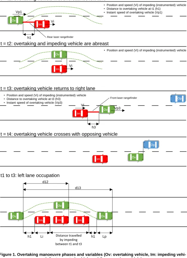
position of overtaking vehicle was measured accurately (see in detail in Figure 1): 219
Time (t1) at the starting time of overtaking manoeuvre (when overtaking vehicle left front 220
wheel crosses the centreline), headway between overtaking and instrumented vehicle 221
(h1) and relative speed (dVp1). 222
Time (t2) at the abreast location (when front bumper of both overtaking and impeding 223
vehicle are at the same point). 224
Time (t3) at the ending time of overtaking manoeuvre (when overtaking vehicle left rear 225
wheel crosses the centreline), headway between overtaking and instrumented vehicle 226
(h3) and relative speed (dVp3). 227
228
229
Figure 1. Overtaking manoeuvre phases and variables (Ov: overtaking vehicle, Im: impeding
vehi-230
cle/instrumented vehicle and Op: opposing vehicle)
231
The values of t1, t2 and t3 were identified by viewing video files of each manoeuvre. Distance 232
between overtaking and impeding vehicle were obtained using the rear laser rangefinder and front 233
laser gun, respectively. Distances travelled along the one-second intervals centred at t1 and t3 234
were considered for the relative speed calculation in order to reduce possible measurement er-235
rors. 236
t = t1: overtaking vehicle first encroaches left lane
• Position and speed (Vi) of impeding (instrumented) vehicle • Distance to overtaking vehicle at t1 (h1)
• Instant speed of overtaking vehicle (Vp1)
Vp1
Vi
h1
t = t2: overtaking and impeding vehicle are abreast
• Position and speed (Vi) of impeding (instrumented) vehicle
Vi
t = t3: overtaking vehicle returns to right lane
t = t4: overtaking vehicle crosses with opposing vehicle
h3• Position and speed (Vi) of impeding (instrumented) vehicle • Distance to overtaking vehicle at t3 (h3)
• Instant speed of overtaking vehicle (Vp3)
Vi Vp3 Ov Ov Ov Ov Im Im Im Im Op Op
Rear laser rangefinder
Front laser rangefinder
Ov Im Im Im Ov Ov h1 Li h1 Lp d12 d13 Distance travelled by impeding between t1 and t3
t1 to t3: left lane occupation
In addition to this, GPS data provided the trajectory of the instrumented impeding vehicle at a 10 237
Hz frequency. Speed of the impeding vehicle Vi was added to the relative speeds to obtain the 238
absolute overtaking vehicle speeds. The distance travelled between t1 and t2 (interval t12) was 239
named d12. The distance travelled from t1 to t3 (interval t13) was named d13. 240
Lastly, the time when overtaking and opposing vehicle crossed each other was called t4. The time 241
interval t34 (equal to t4 –t3) measured the safety margin until the potential collision with the op-242
posing car (Time to Collision). 243
Additional data were also collected from video images and vehicle passenger annotations. The 244
following variables were registered: 245
Type of overtaking vehicle: car, truck. 246
Starting mode: if the overtaking vehicle starts the manoeuvre after following the impeding 247
at the same speed, the manoeuvre is accelerative, if the overtaking vehicles does not 248
reduce the speed prior to overtake, the manoeuvre is flying. 249
Since all the data was obtained using this methodology, it was not possible to know the maximum 250
speed and acceleration that can develop every overtaking vehicle. These data would depend on 251
the power/weight ratio and was not available, due to the naturalistic characteristics of the experi-252
ment, which avoided any intervention during the observations. 253
3.1.3.
Data collection
254
Using the described methodology, 265 overtaking manoeuvres were recorded on five two-lane 255
rural road segments. 256
A total of 85 were discarded due to one or more of the following reasons: 257
Overtaking vehicle was a truck (14 manoeuvres). 258
More than one impeding vehicle was passed (40 multiple manoeuvres). 259
In accelerative manoeuvres, either front, or rear or both laser distance measurements 260
were missing or not valid (52 manoeuvres). 261
In consequence, model calibration was made using only manoeuvres involving one overtaking 262
passenger car and one impeding vehicle (the instrumented vehicle); and with plausible laser 263
measurements at t1 and t3. The selected sample was 151 accelerative overtaking manoeuvres 264
and 29 flying overtaking manoeuvres. 265
No aborted manoeuvres were registered during data collection. Therefore, only completed over-266
taking manoeuvres were modelled. 267
Table 1 summarizes characteristics of road segments and overtaking zones. 268
Road ID Date Design speed
(km/h) Number of manoeu-vres Impeding vehicle speed (Vi, in km/h) N-225 06/02/2012 100 62 80 CV-415 13/09/2012 70 55 60 CV-415 08/11/2012 70 30 60 CV-50 08/11/2012 80 48 70 CV-405 20/11/2012 70 70 60
Table 1. Selected road segments
269
Table 2 shows recorded overtaking manoeuvre variables. First and second rows represent mean 270
and standard deviation of each variable in columns, for accelerative passes. Third and fourth rows 271
show the same for flying passes. 272
Starting mode Variable d12 (m) d13 (m) t12 (s) t13 (s) t34 (s) h1 (m) Vp1 (km/h) h3 (m) Vp3 (km/h) Vi (km/h) Accelera-tive (N = 115) Mean 61.2 163.8 2.9 7.1 4.6 7.5 71.1 21.2 88.8 65.5 SD 19.0 42.0 0.9 1.8 2.0 3.7 10.4 8.2 11.1 8.3 Flying (N = 29)
Mean 70.2 162.5 2.7 6.3 n/a 27.8 n/a 25.2 n/a 64.3 SD 22.1 44.5 0.8 1.6 n/a 14.2 n/a 14.0 n/a 8.4
Table 2. Data summary
273
3.2. Models proposal
274
The aim of this study was the calibration of several overtaking vehicle acceleration models using 275
experimental data. The field study in this research made possible the measurement of more var-276
iables than any other previous studies. In the past, only some authors have recorded the entire 277
trajectory of a passing vehicle. Llorca and Garcia [29] carried out a field study based on external-278
static cameras transforming video images into complete trajectories. The results were limited as 279
this method was very time-consuming. Alternative methods based on instrumented vehicles [22] 280
acting as impeding vehicles did not collect as many data points as the present study, especially 281
because they did not use laser rangefinders. 282
Even using the proposed method, there is still a lack of information between the times t1 and t2, 283
and t2 and t3. This justifies the procedure of fitting different models and compare the calibration 284
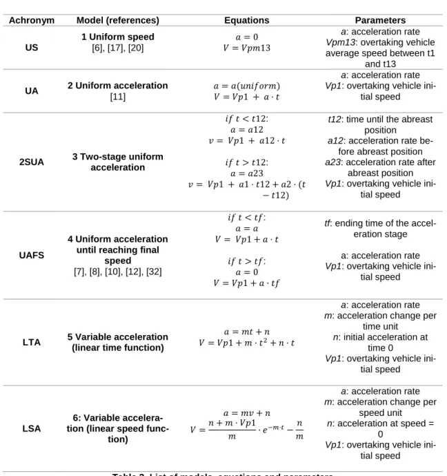
errors among them, as will be explained later. Table 3 shows a list of models, starting with the 285
simplest one (uniform overtaking vehicle speed) and following with more complex approaches. 286
Most of recent existing OSD models in the literature have been included in Table 3. This include 287
new model proposals, too. 288
289 290
Achronym Model (references) Equations Parameters US 1 Uniform speed [6], [17], [20] 𝑎 = 0 𝑉 = 𝑉𝑝𝑚13 a: acceleration rate Vpm13: overtaking vehicle average speed between t1
and t13 UA 2 Uniform acceleration [11] 𝑎 = 𝑎(𝑢𝑛𝑖𝑓𝑜𝑟𝑚) 𝑉 = 𝑉𝑝1 + 𝑎 · 𝑡 a: acceleration rate Vp1: overtaking vehicle
ini-tial speed
2SUA 3 Two-stage uniform acceleration 𝑖𝑓 𝑡 < 𝑡12: 𝑎 = 𝑎12 𝑣 = 𝑉𝑝1 + 𝑎12 · 𝑡 𝑖𝑓 𝑡 > 𝑡12: 𝑎 = 𝑎23 𝑣 = 𝑉𝑝1 + 𝑎1 · 𝑡12 + 𝑎2 · (𝑡 − 𝑡12)
t12: time until the abreast position
a12: acceleration rate be-fore abreast position a23: acceleration rate after
abreast position Vp1: overtaking vehicle
ini-tial speed
UAFS
4 Uniform acceleration until reaching final
speed [7], [8], [10], [12], [32] 𝑖𝑓 𝑡 < 𝑡𝑓: 𝑎 = 𝑎 𝑉 = 𝑉𝑝1 + 𝑎 · 𝑡 𝑖𝑓 𝑡 > 𝑡𝑓: 𝑎 = 0 𝑉 = 𝑉𝑝1 + 𝑎 · 𝑡𝑓
tf: ending time of the accel-eration stage a: acceleration rate Vp1: overtaking vehicle
ini-tial speed
LTA 5 Variable acceleration (linear time function)
𝑎 = 𝑚𝑡 + 𝑛 𝑉 = 𝑉𝑝1 + 𝑚 · 𝑡2+ 𝑛 · 𝑡
a: acceleration rate m: acceleration change per
time unit n: initial acceleration at
time 0
Vp1: overtaking vehicle ini-tial speed
LSA
6: Variable accelera-tion (linear speed
func-tion) 𝑎 = 𝑚𝑣 + 𝑛 𝑉 =𝑛 + 𝑚 · 𝑉𝑝1 𝑚 · 𝑒−𝑚·𝑡− 𝑛 𝑚 a: acceleration rate m: acceleration change per
speed unit n: acceleration at speed =
0
Vp1: overtaking vehicle ini-tial speed
Table 3. List of models, equations and parameters
291 292
293
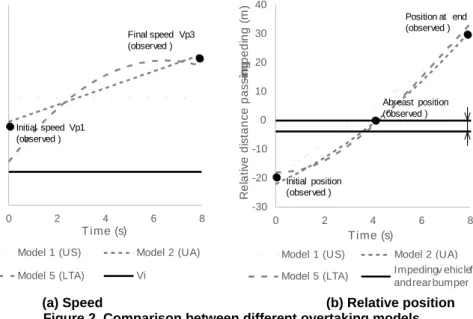
(a) Speed (b) Relative position
Figure 2. Comparison between different overtaking models
294
Figure 2 shows an example of the differences between three of the six alternative models (without 295
scale). Black dots represented measured data points. The use of different models may affect the 296
accuracy in the estimation of initial and final speeds (Figure 2a), and distance travelled at the 297
abreast position and at the end of the overtaking manoeuvre (Figure 2b). As can be seen, the 298
models do not fit the data exactly, but some of them are closer than other ones. This is the basis 299
of the calibration and comparison of up to six models. 300
The real acceleration process depended on driver’s decision and ability, as well as on vehicle 301
performance. The presented models are alternative approaches to describe this process. The 302
potential applications of this study (microsimulation models, probabilistic OSD standards) require 303
the formulation of simple models, where the parameters are defined as random variables. Models 304
were defined as a set of equations, which described the evolution of the overtaking vehicle along 305
its left lane occupation time. 306
3.3. Model calibration
307
Due to overtaking variables randomness, the objective of calibration was to estimate the model 308
parameters for each single overtaking manoeuvre. After that, a probability function of each pa-309
rameter was estimated considering the entire sample. The calibration of models was carried out 310
in two different groups. The first one included only accelerative manoeuvres, since they always 311
involved a positive acceleration starting at a slow speed, near to impeding vehicle speed. A total 312
of 151 overtaking manoeuvres were included in this group. 313
The second group corresponded to flying overtaking manoeuvres. In this case, overtaking vehicle 314
trajectory was very different and starting speed was not necessary so close to impeding vehicle 315
speed as in accelerative passes. On the other hand, during most flying overtaking manoeuvres, 316
no rear distance measurement could be possible, since in those manoeuvres, the value of head-317
way h1 was significantly higher (an average of 27.8 m while it was 7.5 m in accelerative passes) 318
or was out of the laser rangefinder measurement field. A total of 29 manoeuvres were included in 319
the second group. 320
3.3.1.
Accelerative manoeuvres
321
The objective of the calibration of the models of Table 3 was to estimate the value of model 322
parameters, which determine the minimum deviation between estimated and observed overtaking 323 vehicle trajectory. 324 50 60 70 80 90 100 110 0 2 4 6 8 S p e e d ( k m /h ) T ime (s)
Model 1 (US) Model 2 (UA)
Model 5 (LTA) Vi Initial speed Vp1 (observed ) Final speed Vp3 (observed ) -30 -20 -10 0 10 20 30 40 0 2 4 6 8 R e la ti v e d is ta n c e p a s s in g -i m p e d in g ( m ) T ime (s)
Model 1 (US) Model 2 (UA)
Model 5 (LTA) Impeding v ehicle
Abreast position (observed ) Position at end (observed ) Initial position (observed )
(a) Speed (b) Relativ e position Figure 2. Comparison between dif f erent ov ertaking models
Impedingv ehiclef ront and rear bumper
Im p e d in g v e h ic le le n g th
Parameters estimation was performed for each individual overtaking manoeuvre and after that, 325
they were aggregated. For each model and each recorded overtaking manoeuvre the calibration 326
was made by minimizing the function F (Equation 1). This function is defined as a vector of four 327
components. Each component is the relative error in the estimation of each of the overtaking 328 manoeuvre variables. 329
𝐹(𝑋
𝑖, 𝑀
𝑖) =
{
𝑑13𝑚𝑜𝑑𝑒𝑙(𝑀𝑖)−𝑑13𝑜𝑏𝑠𝑒𝑟𝑣𝑒𝑑 𝑑13𝑜𝑏𝑠𝑒𝑟𝑣𝑒𝑑 𝑑12𝑚𝑜𝑑𝑒𝑙(𝑀𝑖)−𝑑12𝑜𝑏𝑠𝑒𝑟𝑣𝑒𝑑 𝑑12𝑜𝑏𝑠𝑒𝑟𝑣𝑒𝑑 𝑉𝑝1𝑚𝑜𝑑𝑒𝑙(𝑀𝑖)−𝑉𝑝1𝑜𝑏𝑠𝑒𝑟𝑣𝑒𝑑 𝑉𝑝1𝑜𝑏𝑠𝑒𝑟𝑣𝑒𝑑 𝑉𝑝3𝑚𝑜𝑑𝑒𝑙(𝑀𝑖)−𝑉𝑝3𝑜𝑏𝑠𝑒𝑟𝑣𝑒𝑑 𝑉𝑝3𝑜𝑏𝑠𝑒𝑟𝑣𝑒𝑑}
(1) 330 Where: 331 𝑋𝑖 = (𝑑13𝑜𝑏𝑠𝑒𝑟𝑣𝑑𝑒𝑑, 𝑑12 𝑜𝑏𝑠𝑒𝑟𝑣𝑒𝑑, 𝑉𝑝1𝑜𝑏𝑠𝑒𝑟𝑣𝑒𝑑, 𝑉𝑝3𝑜𝑏𝑠𝑒𝑟𝑣𝑒𝑑) is a vector of the four 332
observed dynamic variables for manoeuvre i. 333
𝑑13𝑚𝑜𝑑𝑒𝑙, 𝑑12𝑚𝑜𝑑𝑒𝑙, 𝑉𝑝1𝑚𝑜𝑑𝑒𝑙 𝑎𝑛𝑑 𝑉𝑝3𝑚𝑜𝑑𝑒𝑙 are functions of Mi, according to the
se-334
lected model, based on Table 3. 335
𝑀𝑖 = (𝑚𝑖1, 𝑚𝑖2, … 𝑚𝑖𝐾) is a vector of K model parameters for manoeuvre i. 336
Each component of the function corresponded to the difference between the estimated and the 337
observed value of the following variables: distance travelled until t3 (d13), distance travelled until 338
t2 (d12), speed at t1 (Vp1) and speed at t3 (Vp3). These components were divided by the ob-339
served value of each one. The reason of this was to give the same relative importance to all of 340
them. 341
Since number of parameters (between one and three, depending on the model) was lower than 342
number of available data, the equation F = 0 (minimize the error) was solved using least square 343
methods. Both linear and nonlinear least square procedures were applied, (depending on the 344
linearity of model equations), using the Optimization Toolbox included in MATLAB software. The 345
objective of these function was to minimize the terms of the function F(Xi, Mi) according to the
346
Equation 2. 347
𝑀𝑖 /min (𝑓1(𝑋𝑖, 𝑀𝑖)2+ 𝑓2(𝑋𝑖, 𝑀𝑖)2+ 𝑓3(𝑋𝑖, 𝑀𝑖)2+ 𝑓4(𝑋𝑖, 𝑀𝑖)2) for i=1 to N (2)
348
Where: 349
𝑋𝑖 = (𝑑13𝑜𝑏𝑠𝑒𝑟𝑣𝑑𝑒𝑑, 𝑑12 𝑜𝑏𝑠𝑒𝑟𝑣𝑒𝑑, 𝑉𝑝1𝑜𝑏𝑠𝑒𝑟𝑣𝑒𝑑, 𝑉𝑝3𝑜𝑏𝑠𝑒𝑟𝑣𝑒𝑑) is a vector of the four 350
observed kinematic variables for manoeuvre i. 351
𝑑13𝑚𝑜𝑑𝑒𝑙, 𝑑12𝑚𝑜𝑑𝑒𝑙, 𝑉𝑝1𝑚𝑜𝑑𝑒𝑙 𝑎𝑛𝑑 𝑉𝑝3𝑚𝑜𝑑𝑒𝑙 are functions of Mi, according to the
se-352
lected model, based on Table 3. 353
𝑀𝑖 = (𝑚𝑖1, 𝑚𝑖2, … 𝑚𝑖𝐾) is a vector of K model parameters for manoeuvre i. 354
𝑁 is the number of manoeuvres. 355
For each model, parameter probability distributions were analysed after aggregating all manoeu-356
vres. Table 4 summarizes the probability distribution of each parameter as well as existing corre-357
lations between different parameters. In every case, the distribution fitting was checked using 358
both Chi-Square and Kolmogorov-Smirnov tests. Correlations between model parameters have 359
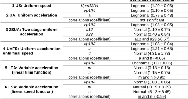
been analysed. Table 4 includes significant correlations (over 0.5) at the 95% confidence level. 360
Model Parameters Distribution and values (mean ±SD) Correlation coefficients
1 US: Uniform speed Vpm13/Vi Lognormal (1.20 ± 0.06)
2 UA: Uniform acceleration
Vp1/Vi Lognormal (1.10 ± 0.05) a Lognormal (0.77 ± 0.48) correlations (coefficient) not significant
3 2SUA: Two-stage uniform acceleration
Vp1/Vi Lognormal (1.08 ± 0.05) a12 Normal (1.19 ± 0.74) a23 Normal (0.40 ± 0.54) correlations (coefficient) a12 and a23 (-0.57)
4 UAFS: Uniform acceleration until final speed
Vp1/Vi Lognormal (1.08 ± 0.04) a Lognormal (1.31 ± 0.68) tf Normal (4.31 ± 1.73) correlations (coefficient) a and tf (-0.66)
5 LTA: Variable acceleration (linear time function)
Vp1/Vi Lognormal (.08 ± 0.05)
m Normal (0.13 ± 0.18)
n Normal (1.15 ± 0.75) correlations (coefficient) m and n (-0.90)
6 LSA: Variable acceleration (linear speed function)
Vp1/Vi Normal (1.08 ± 0.05) m Normal (-0.19 ± 0.29)
n Normal (5.13 ± 6.45) correlations (coefficient) m and n (-0.99)
Table 4. Results of model calibration for accelerative passes
362
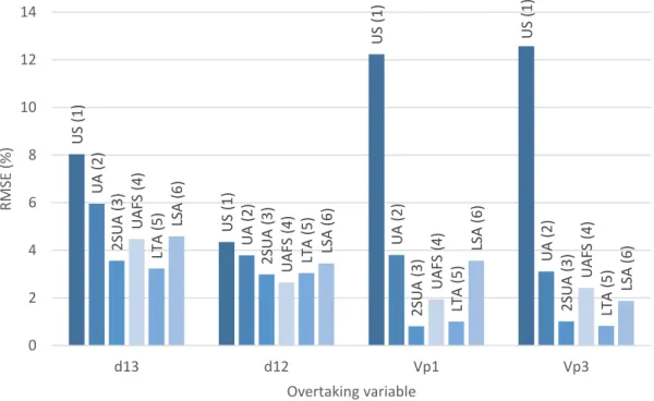
Figure 3 represents the percent root mean squared error (RMSEj) for each calibration variable j 363
and model. RMSE was calculated using the Equation 3. 364 𝑅𝑀𝑆𝐸𝑗 = √1𝑁∑ (𝑓𝑖𝑗) 2 𝑁 𝑖=1 (3) 365
Where fij is the relative error of variable j in the manoeuvre i, corresponding to a term of the 366
function f(Xi, Mi). 367
As can be seen, increasing model complexity, the estimation errors generally decrease, since 368
models 3 (2SUA), 4 (UAFS) and 5 (LTA) had the lowest errors for each variable. In Figure 4, 369
models are ranked according to the percentage of cases in which they are the best (and the 370
second best) fitted model, according to the RMSE. It means, in example, that model 3 (2SUA) 371
was the best model for 28% of the cases and was in the second place for 26%. 372
373
Figure 3. Root mean square error (percent) for each model and variable
374
375
Figure 4. Best fit model
376
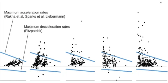
For each case, the estimated acceleration values were checked, in order to proof if the calibration 377
resulted in abnormal values. Reference maximum acceleration rates were Rakha et al. [33], 378
Sparks et al. [14] , and Liebermann [13]; reference deceleration rates were Fitzpatrick et al. [34]. 379
These reference values determined whether an acceleration value exceed the reasonable rates 380
or not. Figure 5 shows the range of reasonable acceleration rates, as well as the estimated values 381
for each model, depending on the overtaking vehicle speed. Acceleration rates among lower and 382
upper thresholds were considered as valid. Otherwise, they were discarded. 383 U S (1) U S (1) U S (1) U S (1) U A (2) U A (2) U A (2) U A (2) 2SU A (3) 2SU A (3) 2SU A (3) 2SU A (3) U AFS (4) U AFS (4) U AFS (4) U AFS (4) LT A (5) LT A (5) LT A (5) LT A (5) LSA (6) LSA (6) LSA (6) LSA (6) 0 2 4 6 8 10 12 14 d13 d12 Vp1 Vp3 RMSE (% ) Overtaking variable 11% 28% 29% 19% 13% 8% 6% 26% 17% 30% 13% 0% 10% 20% 30% 40% 50% 60%
US (1) UA (2) 2SUA (3) UAFS (4) LTA (5) LSA (6)
Ma n o eu vre s (% ) Model
384
Figure 5. Acceleration (positive values) and deceleration (negative values) rate thresholds vs.
esti-385
mated values
386
By increasing model complexity, some observed manoeuvres provided non-feasible solutions, as 387
can be seen in Figure 6. Those manoeuvres were discarded when analysing parameter distribu-388
tions of Table 4. Models with a high number of discarded manoeuvres could not be able to explain 389
overtaking vehicle behaviour. This case could be associated to overfitting, since the models rep-390
resented very well the three data points but not properly the rest of the trajectory. 391
392 393
394
Figure 6. Non-feasible solutions for each model
395
3.3.2.
Flying manoeuvres
396
Flying overtaking manoeuvres represented a different behaviour, compared to accelerative 397
passes. OSD requirements are usually lower for flying passes so they are not considered in many 398
manoeuvre models [6]–[8]. Flying passes do not involve necessarily an acceleration process, 399
because overtaking vehicle speed is higher once the manoeuvre has started. 400 15 25 35 model 4: UAFS 15 25 35 model 3: 2SUA -4 -2 0 2 4 6 8 10 12 14 16 18 15 25 35 A c c e ler a tion ( m /s 2) model 2: UA 15 25 35 model 5: LTA Overtaking vehicle speed (m/s)
15 25 35
model 6: LSA
Maximum acceleration rates
(Rakha et al, Sparks et al. Liebermann) Maximum decceleration rates (Fitzpatrick) 0 0 20 18 36 42 0 5 10 15 20 25 30 35 40 45
US (1) UA (2) 2SUA (3) UAFS (4) LTA (5) LSA (6)
N u m b er o f n o n -f easi b le s o lu tio n s Model
Only one model was calibrated for the flying manoeuvres observed using the experimental meth-401
odology. It was the model 1 (US), corresponding to an overtaking vehicle travelling at a uniform 402
speed. This selection was made due to the two following reasons: 403
According to the definition of flying manoeuvre, the overtaking vehicle neither brakes nor 404
accelerates, accepting an overtaking gap just after reaching the impeding vehicle. 405
Overtaking vehicle trajectory measurement was more difficult in flying manoeuvres than 406
in accelerative, since headways h1 and h3 were longer. In most cases, it was not possible 407
to measure the overtaking vehicle speed at t1 and t3. Therefore, it was impossible to 408
calibrate more complex models. 409
The calibration of this model was based on data from 29 manoeuvres observed with the instru-410
mented vehicle. Despite headways h1 and h3 could not be measured using the laser rangefind-411
ers, they were estimated from video images. This estimation was based on drawing reference 412
lines on video frames at known distances, as proposed previously by Carlson et al [22] Those 413
reference points were measured and recorded on video images before starting data collection. 414
Accuracy of those measurements was lower, and it was not possible to calculate reliable instant 415
speeds at t1 or t3. 416
The model 1 was calibrated minimizing the error of the distances d12 and d13, using the same 417
procedure as for accelerative overtaking manoeuvres. Percent RMSE was 5% for both d12 and 418
d13 distances. Table 5 shows the distribution of adjusted parameters. 419
Model Adjusted parameters Distribution & Values (mean ± SD)
1 Uniform speed Vpm13/Vi Normal (1.43 ± 0.10)
Table 5. Parameters of overtaking model for flying manoeuvres.
420
4. Results
421
The results of the calibration showed that the use of different models involved significant differ-422
ences in the estimation of overtaking vehicle trajectories. 423
Simpler models, such as model 1 (US) were not able to explain the speed evolution during the 424
left lane occupation, in the case of accelerative manoeuvre. The RMSE of this model was over 425
10% in initial and final speeds, and of 8 and 4% in distance d13 and d12, respectively. According 426
to the model calibration, the average speed of the overtaking vehicle would be a 20% higher than 427
the impeding vehicle speed. 428
Models 2 (UA), 3 (2SUA) and 4 (UAFS) were more adequate (in terms of RMSE) to estimate both 429
d13 and d12, as well as initial and final speeds Vp1 and Vp3. Model 2 (UA) explained the ma-430
noeuvre with a uniform acceleration movement during t13. Model 3 (2SUA) incorporated two 431
stages with different acceleration rates, in order to represent the potential change in the acceler-432
ation rate once the abreast position was reached. Model 4 (UAFS) was similar to model 3, alt-433
hough it assumed, based on previous research studies, that the overtaking vehicle accelerated 434
until a final speed was reached, keeping this speed after that. The models 2, 3 and 4 presented 435
a low percent RMSE for the calibration variables, being always under 5%. 436
Model 5 (LTA) incorporated an additional term to represent a linear variation of the acceleration 437
rate as a function of time. Model 6 (LSA) was based also in a linear variation, but as a function of 438
the speed, according to Rakha et al. [33] acceleration profiles. The most complex models were 439
not adequate to represent the entire observed data. The models 5 and 6 calibration process had 440
as a result a relative high number of not feasible solutions, characterized by excessively high (or 441
low) acceleration rates. 442
In models 2 to 6, the initial speed of the overtaking vehicle Vp1 was, on average, between a 7% 443
and 10% higher than the impeding vehicle speed, which revealed that an initial acceleration was 444
performed before starting the overtaking manoeuvre. After this point, the different models showed 445
different acceleration rates. The model 2 (UA) was characterized a mean uniform acceleration of 446
0.77 m/s2. The model 3 (2SUA) defines two stages: before the abreast position, the mean
accel-447
eration rate was 1.18 m/s2, while after this point it decreased until 0.40 m/s2. The model 4 (UAFS)
448
showed an equivalent result, being the mean acceleration rate of 1.3 until the time tf, when it 449
became zero. The mean time tf was 0.75 times t13. 450
According to model 5 (LTA), an average behaviour was characterized an acceleration rate starting 451
at 1.15 m/s2 and decreasing 0.13 m/s2 per second. The model 6 (LSA) explains the average
452
behaviour by an acceleration rate following the relationship 𝑎 = 5.13 – 0.19𝑣 (v in m/s and a in 453
m/s2).
454
A general conclusion is that an average behaviour of overtaking drivers could be modelled by a 455
decreasing acceleration rate during the overtaking time t13. The reason behind this could be, 456
firstly, that maximum acceleration capacity decreased when speed increases, and second, that 457
drivers might reduce their acceleration rate as far as they observe that the manoeuvre can be 458
completed with safety. 459
On the other hand, the model 1 (US) was able to explain how a flying manoeuvre was performed. 460
In this case, it had a percent RMSE under 5% in both d12 and d13. 461
5. Discussion
462
This research study have compared previously existing overtaking models with observational data 463
of overtaking manoeuvres on a sample of two-lane rural roads in the surrounding of Valencia 464
(Spain). Validity of results should be initially limited to this geographical area, as drivers’ behaviour 465
may be different in other regions or countries. Model 1 (US) was equivalent to the previous 466
AASHTO Green Book model [6]. This model could not account for the overtaking vehicle speed 467
variation in accelerative overtaking manoeuvres, since only a uniform speed was considered. 468
Model 2 (UA) was equal to the one proposed by Rocci [11]. This author proposed an acceleration 469
value ranging between 0.27 and 2.17 m/s2, with a 50th percentile of 1.11 m/s2. These values are
470
slightly higher than the observed distribution. Besides, Rocci assumed that the initial speed of 471
overtaking vehicle was equal to the impeding vehicle speed. This was not observed in the present 472
study data. 473
Model 4 (UAFS) is similar to Glennon [7] and Hassan et al. [8] although those authors proposed 474
that the overtaking vehicle speed was uniform after the critical point. The model in the present 475
paper was calibrated assuming that the uniform speed started at a certain point (calibrated as 476
well) during the overtaking manoeuvre, since it is not possible to measure the critical point on the 477
field (with any type of equipment). Besides, the uniform speed, among all the other parameters 478
including the final point of the acceleration phase, were assumed to be random variables. The 479
results of the calibration showed that, in contrast to Glennon and Hassan et al. models, the over-480
taking vehicle speed at the starting point of the manoeuvre was not equal to the impeding vehicle 481
speed. Moreover, the final speed was a random variable 10 km/h (on average) over the design 482
speed of the observed roads. 483
In relation to the acceleration rates, the AASHTO [6] model proposed similar mean values (around 484
0.62 m/s2) to those obtained from model 2 (UA) (50th percentile at 0.70 m/s2). The AASHTO
485
model defined the acceleration stage before entering the left lane, though. If extreme acceleration 486
rates are analysed, the 85th percentile obtained from Model 2 (2.25 m/s2) was close to those
487
observed by Rakha et al. [33] and to those proposed by Sparks et al. [14] at the equivalent speed 488
levels (shown in Figure 5). Similarly Basilio et al. [3] assumed a uniform acceleration model as 489
upper threshold for the driving simulator vehicles. The value of maximum acceleration for the 490
lower speed vehicle (100 km/h) was close to the 85th percentile of observations (2 m/s2).
6. Conclusion
492
The characterization of the trajectory of overtaking vehicles travelling on the opposing lane is 493
fundamental to calculate the left lane occupation time; which is the main variable used to calibrate 494
and further develop of ADAS, as well as to improve geometric design and marking guidelines for 495
two-lane rural roads. The values of overtaking time provide the sight distance requirements to 496
perform a safe and comfortable manoeuvre, taking into account the opposing flow. 497
This research characterized the trajectory of 180 overtaking vehicles by using kinematic models, 498
which were calibrated from observations of the real phenomenon. The main conclusions were: 499
500
Accelerative overtaking manoeuvres should be represented by a model that considers 501
acceleration during the left lane occupation phase. A uniform acceleration model with an 502
average rate of 0.77 m/s2 is recommended for them, balancing accuracy and simplicity.
503
The acceleration rate is log-normal distributed. 504
Flying overtaking manoeuvres are adequately represented by a uniform speed model. 505
The speed on left lane is normal distributed, centred on an average value of 1.43 times 506
of the speed of the impeding vehicle. 507
The ability of these models to predict the manoeuvre duration, travelled distance and abreast 508
position was assessed. However, the extrapolation of this results should be taken with caution, 509
since drivers’ behaviour may be different in other geographical areas. The application of the re-510
sults to overtaking manoeuvres when the overtaken vehicle is a truck should be verified by addi-511
tional observations. 512
Despite the above mentioned limitations, the development of ADAS should combine the results 513
of this paper, as a model to predict overtaking vehicle trajectories, with the maximum capacities 514
of the vehicles (acceleration) as well as the input of the current conditions (mainly the distance 515
and speed of the opposing vehicle). 516
The selection of the best model would depend on its intended applications. Potential applications 517
are the review of road design and marking guidelines, the calibration of traffic microsimulation 518
models and the development or calibration of assistance systems, either based on autonomous 519
driving controllers, or warning devices or mapping and geographical information systems. 520
7. Acknowledgments
521
Part of this research was included in the project “Desarrollo de modelos de distancias de visi-522
bilidad de adelantamiento”, with reference code TRA2010-21736 and subsidized by the Spanish 523
Ministery of Economy and Competitivity. Authors would also like to thank Prof. Dr. Sayed, from 524
University of British Columbia, for his valuable review. 525
8. References
526 527
[1] A. Molinero, E. Carter, C. Naing, M. Simon, and T. Hermintte, “Accident causation and 528
pre-accidental driving situations. Part 1. Overview and general statistics, TRACE - Traffic 529
Accident Causation in Europe Report,” 2008. 530
531
[2] R. Gray and D. M. Regan, “Perceptual processes used by drivers during overtaking in a 532
driving simulator.,” Human factors, vol. 47, no. 2, pp. 394–417, 2005. 533
534
[3] N. Basilio, a. H. P. Morice, G. Marti, and G. Montagne, “High- and Low-Order Overtaking-535
Ability Affordances: Drivers Rely on the Maximum Velocity and Acceleration of Their Cars 536
to Perform Overtaking Maneuvers,” Human factors, vol. 57, no. 5, pp. 879–894, 2015. 537
538
[4] A. H. P. Morice, G. J. Diaz, B. R. Fajen, N. Basilio, and G. Montagne, “An Affordance-539
Based Approach to Visually Guided Overtaking,” Ecological Psychology, vol. 27, no. 1, 540
pp. 1–25, 2015. 541
542
[5] H. Farah, S. Bekhor, and A. Polus, “Risk evaluation by modeling of passing behavior on 543
two-lane rural highways.,” Accident; analysis and prevention, vol. 41, no. 4, pp. 887–94, 544
Jul. 2009. 545
546
[6] American Association of State Highway and Transportation Official, A Policy on Geometric 547
Design of Highways and Streets, 5th Edition. 2004. 548
549
[7] J. C. Glennon, “New and improved model of passing sight distance on two-lane highways,” 550
Transportation Research Record: Journal of the Transportation Research Board, no. 551
1195, pp. 132–137, 1988. 552
553
[8] Y. Hassan, S. M. Easa, and A. O. A. El Halim, “Passing sight distance on two-lane 554
highways: Review and revision,” Transportation Research Part A: Policy and Practice, vol. 555
30, no. 6, pp. 453–467, Nov. 1996. 556
557
[9] Federal Highway Administration, Manual on Uniform Traffic Control Devices. 2009. 558
559
[10] American Association of State Highway and Transportation Official, A Policy on Geometric 560
Design of Highways and Streets, 6th Edition. 2011. 561
562
[11] S. Rocci, “A system for no passing zones signing and marking setup,” in Transportation 563
Research Board Circular, 1998. 564
565
[12] Y. Wang and M. P. Cartmell, “New model for passing sight distance on two-lane 566
highways,” Journal of Transportation Engineering, vol. 124, no. 6, pp. 536–544, 1998. 567
568
[13] E. B. Lieberman, “Model for Calulculating Safe Passing Distances on Two-Lane Rural 569
Roads,” Transportation Research Record: Journal of the Transportation Research Board, 570
vol. 1280, pp. 70–76, 1982. 571
572
[14] B. G. A. Sparks, R. D. Neudorf, J. B. L. Robinson, and D. Good, “Effect Of Vehicle Length 573
On Passing Operations,” Journal of Transportation Engineering, vol. 119, no. 2, 1993. 574
575
[15] P. F. Hanley and D. J. Forkenbrock, “Safety of passing longer combination vehicles on 576
two-lane highways,” Transportation Research Part A: Policy and Practice, vol. 39, no. 1, 577
pp. 1–15, Jan. 2005. 578
579
[16] J. El Khoury and A. G. Hobeika, “Integrated Stochastic Approach for Risk and Service 580
Estimation : Passing Sight Distance Application,” Journal of Transportation Engineering, 581
pp. 571–579, 2012. 582
[17] S. El-bassiouni and T. Sayed, “Design Requirements for Passing Sight Distance : A Risk-584
based Approach,” in 90th Transportation Research Board Annual Meeting, 2010. 585
586
[18] J. M. Jenkins and L. R. Rilett, “Application of distributed traffic simulation for passing 587
behavior study,” in Transportation Research Record, 2004, no. 1899, pp. 11–18. 588
589
[19] H. Rakha, K. Ahn, and A. Trani, “Development of VT-Micro model for estimating hot 590
stabilized light duty vehicle and truck emissions,” Transportation Research Part D: 591
Transport and Environment, vol. 9, no. 1, pp. 49–74, Jan. 2004. 592
593
[20] A. Polus, M. Livneh, and B. Frischer, “Evaluation of the Passing Process on Two-Lane 594
Rural Highways,” Transportation Research Record: Journal of the Transportation 595
Research Board, vol. 1701, pp. 53–60, 2000. 596
597
[21] D. W. Harwood, D. K. Gilmore, and K. R. Richard, “Passing Sight Distance Criteria for 598
Roadway Design and Marking,” Transportation Research Record: Journal of the 599
Transportation Research Board, vol. 2195, pp. 36–46, 2010. 600
601
[22] P. Carlson, J. Miles, and P. Johnson, “Daytime High-Speed Passing Maneuvers Observed 602
on Rural Two-Lane, Two-Way Highway: Findings and Implications,” Transportation 603
Research Record, vol. 1961, no. 1, pp. 9–15, Jan. 2006. 604
605
[23] G. Hegeman, Assited Overtaking, An Assessment of Overtaking on Two-Lane Rural 606
Roads. PhD Thesis. TU Delft, 2008. 607
608
[24] G. Hegeman, A. Tapani, and S. Hoogendoorn, “Overtaking assistant assessment using 609
traffic simulation,” Transportation Research Part C: Emerging Technologies, vol. 17, no. 610
6, pp. 617–630, Dec. 2009. 611
612
[25] V. Milanés, D. F. Llorca, J. Villagrá, J. Pérez, C. Fernández, I. Parra, C. González, and M. 613
A. Sotelo, “Intelligent automatic overtaking system using vision for vehicle detection,” 614
Expert Systems with Applications, vol. 39, no. 3, pp. 3362–3373, Feb. 2012. 615
616
[26] R. Isermann, R. Mannale, and K. Schmitt, “Collision-avoidance systems PRORETA: 617
Situation analysis and intervention control,” Control Engineering Practice, vol. 20, pp. 618
1236–1246, 2012. 619
620
[27] P. Petrov and F. Nashashibi, “Modeling and nonlinear adaptive control for autonomous 621
vehicle overtaking,” IEEE Transactions on Intelligent Transportation Systems, vol. 15, no. 622
4, pp. 1643–1656, 2014. 623
624
[28] J. Loewenau, K. Gresser, and D. Wisselmann, “Dynamic Pass Prediction – A New Driver 625
Assistance System,” in Advanced Microsystems for Automotive Applications, Springer, 626
Ed. 2006, pp. 67–77. 627
628
[29] C. Llorca and A. García, “Evaluation of Passing Process on Two-Lane Rural Highways in 629
Spain with New Methodology Based on Video Data,” Transportation Research Record: 630
Journal of the Transportation Research Board, vol. 2262, no. -1, pp. 42–51, Dec. 2011. 631
[30] C. Llorca, A. T. Moreno, A. García, and A. M. Pérez-Zuriaga, “Daytime and Nighttime 633
Passing Maneuvers on a Two-Lane Rural Road in Spain,” Transportation Research 634
Record: Journal of the Transportation Research Board, vol. 2358, no. -1, pp. 3–11, Dec. 635
2013. 636
637
[31] C. Llorca, A. García, A. T. Moreno, and A. M. Pérez-Zuriaga, “Influence of age, gender 638
and delay on overtaking dynamics,” IET Intelligent Transport Systems, vol. 7, no. 2, pp. 639
174–181, Jun. 2013. 640
641
[32] J. El Khoury and A. Hobeika, “Incorporating Uncertainty into the Estimation of the Passing 642
Sight Distance Requirements,” Computer-Aided Civil and Infrastructure Engineering, vol. 643
22, no. 5, pp. 347–357, Jul. 2007. 644
645
[33] H. Rakha, M. Snare, and F. Dion, “Vehicle Dynamics Model for Estimating Maximum Light-646
Duty Vehicle Acceleration Levels,” Transportation Research Record, vol. 1883, no. 1, pp. 647
40–49, Jan. 2004. 648
649
[34] K. Fitzpatrick, S. T. Chrysler, and M. Brewer, “Deceleration Lengths for Exit Terminals,” 650
Journal of Transportation Engineering, no. June, pp. 768–775, 2012. 651