Efficiently Solving Repeated Integer Linear Programming Problems by Learning Solutions of Similar Linear Programming Problems using Boosting Trees

MIT-CSAIL-TR-2015-001

January 21, 2015

Efficiently Solving Repeated Integer

Linear Programming Problems by

Learning Solutions of Similar Linear

Programming Problems using Boosting Trees

Efficiently Solving Repeated Integer Linear Programming Problems

by Learning Solutions of Similar Linear Programming Problems using

Boosting Trees

Ashis Gopal Banerjee ASHIS@CSAIL.MIT.EDU

Computer Science and Artificial Intelligence Laboratory Massachusetts Institute of Technology

Cambridge, MA 02139, USA

Nicholas Roy NICKROY@CSAIL.MIT.EDU

Computer Science and Artificial Intelligence Laboratory Massachusetts Institute of Technology

Cambridge, MA 02139, USA

Abstract

It is challenging to obtain online solutions of large-scale integer linear programming (ILP) problems that occur frequently in slightly different forms during planning for autonomous systems. We refer to such ILP problems as repeated ILP problems. The branch-and-bound (BAB) algorithm is commonly used to solve ILP problems, and a significant amount of computation time is expended in solving numerous relaxed linear programming (LP) problems at the nodes of the BAB trees. We observe that the relaxed LP problems, both within a particular BAB tree and across multiple trees for repeated ILP problems, are similar to each other in the sense that they contain almost the same number of constraints, similar objective function and constraint coefficients, and an identical number of decision variables. We present a boosting tree-based regression technique for learning a set of functions that map the objective function and the constraints to the decision variables of such a system of similar LP problems; this enables us to efficiently infer approximately optimal solutions of the repeated ILP problems. We provide theoretical performance guarantees on the predicted values and demonstrate the effectiveness of the algorithm in four representative domains involving a library of benchmark ILP problems, aircraft carrier deck scheduling, vehicle routing, and vehicle control.

Keywords: Combinatorial optimization, linear programming, regression, boosting trees, planning 1. Introduction

Combinatorial optimization plays a vital role in many planning problems for autonomous systems ranging from flexible manufacturing cells to unmanned vehicles. The branch-and-bound (BAB) al-gorithm is popularly used to solve integer linear programming (ILP) problems that occur frequently in such optimization problems. Although commercial solvers such as CPLEX and open-source software libraries like COIN-OR (Lougee-Heimer, 2003) provide efficient implementations, it takes minutes to hours to compute the solutions of ILP problems involving tens of thousands of decision variables and comparable number of constraints. Moreover, the solution needs to be recomputed from scratch even when only a small fraction of the problem data (constraint and objective function coefficients) change as more information becomes available in uncertain environments. We refer to

such large-scale ILP problems that arise multiple times in slightly different forms asrepeatedILP problems.

A representative example domain is that of airport operations, where hundreds of flights of many different types need to take off and land safely every day with as few delays as possible. Each type of aircraft has a different fuel consumption rate, refueling time, aerial and ground speeds. Since the airport has a limited number of resources (landing strips, launching zones, parking spots, refueling stations, crew members to assist in loading and unloading of baggage etc.), a large number of con-straints are imposed on the system. Planning such an operation can be conveniently posed as an ILP problem, where the objective is to minimize the disruption in the nominal schedule of each aircraft while satisfying all the system constraints. An optimum plan can be generated by solving this huge ILP problem offline using hours of computation. However, the environmental conditions are subject to frequent but rarely drastic changes. For example, worse weather conditions may render certain launching zones or landing strips unusable, or increase the fuel burn rates of the aircraft. Mechan-ical or hydraulic failures in an airborne aircraft may force it to make an emergency landing. In all such cases, the pre-computed plans cannot be used, and new plans have to be generated on-the-fly.

Since it is not possible to compute exactly optimal plans for quick response to dynamic envi-ronmental conditions corresponding to repeated ILP problems, we need approximate ILP solvers. Even though many approximation algorithms and parametric techniques are available in the litera-ture, they do not specifically leverage the similarity among the repeated ILP problems. Hence, they cannot quickly estimate near-optimal solutions of problems that are often similar to many other repeated ILP problems for which optimal solutions have been already computed. Moreover, they are often designed for a specific class of ILP problems such as routing, packing, or covering. As a result, they are unable to provide desirable performance for a wide variety of problem domains.

Solving any ILP problem using the BAB algorithm involves solving a large number of relaxed linear programming (LP) problems at the BAB tree nodes, where both the objective function and the constraints are linear functions of continuous-valued decision variables that do not have to be integers. The relaxed LP problems often share multiple common constraints and always contain the same decision variables. Especially in the case of repeated ILP problems, often the decision vari-ables do not change, only some of the objective function and constraint coefficient values change, and a few constraints are added or deleted. Henceforth, we refer to LP problems that contain the same decision variables, and similar objective function and constraint coefficients with some varia-tion in the number of equality constraints as a set ofsimilarLP problems.

We observe that the solutions of similar LP problems are usually quite similar themselves in the sense that most of the optimal decision variable values do not change much from one problem to another. Since the optimal values lie at the intersection of the active constraints for any LP problem, our observation indicates that the set of active constraints also do not vary much for similar LP problems. Hence, there is an opportunity to use supervised learning for inferring the correct set of active constraints, and consequently the optimal solution, for any new (test) LP problem by leveraging its similarity with other LP problems present in the training phase. We show that regression can, indeed, be effectively applied to rapidly estimate the optimal LP solutions instead of computing them exactly using a standard optimization solver. Thus, this technique provides a practically useful approach for solving repeated ILP problems online.

More specifically, in this paper, we define the concept of similarity for LP problems and present a boosting tree-based approach, called the Boost-LP algorithm, to learn a set of regression functions that map the objective function and constraints to the individual decision variables of similar LP

problems. We provide absolute performance guarantees in terms of deviations from the optimal for both the LP problem objective function and the individual decision variable values. We then use the objective function performance bounds to prune BAB tree paths while solving the overall ILP problem. We also empirically demonstrate the effectiveness of our algorithm in a collection of benchmark ILP problems, aircraft carrier deck scheduling, vehicle routing, and some well-studied vehicle control problems. The algorithm achieves marked computational speed-up (up to 100 times) as compared to the popular optimization solvers, and obtains promising results with respect to the quality of the overall ILP solutions as the mean deviations of the predicted objective function values are not more than 5% from the true optimal.

2. Related Work

Computing approximately optimal solutions of combinatorial optimization problems in general, and ILP problems in particular, has received a great deal of attention in the literature. The available techniques can be broadly classified into four categories: machine learning, evolutionary optimiza-tion, metaheuristics, and multiparametric programming. We now discuss some of the representative work in each of these categories along with a brief summary of their limitations, and conclude by outlining the goals of the current research in addressing some of the shortcomings.

Machine learning: Zhang and Dietterich (1996) applied temporal difference learning to job shop scheduling using a time-delay neural network architecture to learn search heuristics for obtaining close-to-optimal schedules in shorter periods of time than using the previous non-learned heuris-tics. However, the factor of improvement in computation speed was relatively modest. Lee et al. (1997) used decision trees for scheduling release of jobs into the shop floor and a genetic algorithm (GA) for allocating jobs to the machines and obtained promising results as compared to the con-ventional single release and allocation approach for 3-7 workstations. Telelis and Stamatopoulos (2001) applied a kernel regression-supported heuristic methodology in knapsack and set partition-ing problems and obtained solution qualities of about 60% (measured with respect to the optimal) for constraint matrices involving up to 6000 rows and 25 columns. Vladuˇsiˇc et al. (2009) employed locally weighted learning, na¨ıve Bayes, and decision trees for job shop scheduling over heteroge-nous grid nodes in conjunction with baseline round-robin, random, and FIFO algorithms to obtain improvements over using the baseline algorithms on their own for tasks involving 1000 jobs. We can summarize that although machine learning approaches provide a promising research direction, further work is needed to enhance the computational speed-up factor, and the ability to solve larger-sized problems involving tens of thousands of decision variables (instead of thousands) for a wide variety of problem domains.

Evolutionary optimization: Evolutionary techniques have been most popularly used for solving the class of vehicle routing problems (VRP), where a number of cities must be traversed just once by one or more vehicles, all of which must return to the originating cities. The optimum solution is the set of routes that minimizes the total distance traveled. Representative examples include a genetic algorithm to solve the multi-VRP (involving multiple vehicles) developed in Louis et al. (1999), an ant colony optimization method to search for multiple routes of the VRP presented in Bell and McMullen (2004), and a combination ofk-means clustering and genetic algorithm to solve the multi-VRP proposed in Nallusamy et al. (2009). These approaches have had mixed success as

none of them work uniformly well for problems of varying sizes and types, and the benefit in terms of computational savings is not that large.

Metaheuristics: Metaheuristic techniques have been widely used to solve a variety of combi-natorial optimization problems, and the most common technique for ILP problems is known as LP rounding. Rounding refers to the process of obtaining integral solutions from fractional values of the decision variables. Rounding techniques can be broadly classified into two types: those that round variables non-deterministically (known as randomized rounding) and those that perform rounding deterministically. Within randomized rounding (RR), notable works include the basic approach proposed in Raghavan and Thompson (1987), Raghavan (1988), and Srinivasan (1999) for packing, routing, and multicommodity flow problems, the variant developed in Goemans and Williamson (1994) for the maximum satisfiability problem, and the combination of RR with semidefinite pro-gramming in Goemans and Williamson (1995) for the maximum cut problem. Other key works include simultaneously rounding a set of variables in Bertsimas et al. (1999) for the maximum cut problem, better handling of the equality constraints in Arora et al. (2002) for dense graph problems, and randomized metarounding in Carr and Vempala (2002) for the multicast congestion problem. Within deterministic rounding, representative works include iterated rounding in Jain (2001) for the generalized Steiner network problem, conditional expectation in Chudak and Shmoys (2003) for the uncapacitated facility location problem, and pipage rounding in Ageev and Sviridenko (2004) for the maximum coverage problem. We refer the reader to Chapter 7 in Gonzalez (2007) and Chapters 4 and 5 in Williamson and Shmoys (2011) for a much more comprehensive survey of all the avail-able rounding techniques. Although rounding approaches provide useful performance bounds on several types of ILP problems, no single approach is found to work well on all types of problems. Moreover, all of these approaches obtain exactly optimal solutions of LP problems, and, hence, even though they have polynomial time complexities, they do not provide orders of magnitude reduction in actual computation times.

Multiparametric programming: Another class of ILP solution techniques that is related to our work is multiparametric programming. In multiparametric programming, the optimization problem data are functions of multiple parameters. This technique provides a valuable tool to analyze the effect of variations in optimization problems that arise due to model uncertainties, and has been popularly used in the context of process scheduling and model predictive control. The effects of parameterizing the objective function and the right-hand side of the constraint equations are most commonly studied in the literature. One of the earliest solution methods was proposed in Gal and Nedoma (1972), who partitioned the parameter space into critical regions such that there is one op-timal solution for all the LP problems that are parameterized within each region. Later on, several approaches have been developed that extend the previous method using, for example, a geometric representation Adler and Monteiro (1992), a recursive construction of the critical regions Borrelli et al. (2003), or a linear interpolation based approximate generation of the critical regions Filippi (2004). With respect to multiparametric ILP problems, Dua and Pistikopoulos (2000) decomposed the overall problem into a multiparametric LP problem with fixed values of the integer variables and a mixed ILP with the parameters treated as variables. Li and Ierapetritou (2007) developed an-other decomposition technique, wherein each sub-problem encodes the information around a given parameter value and is then solved using a series of multiparametric LP and mixed integer linear or non-linear programming problems. We refer the interested reader to Pistikopoulos et al. (2007) and Alessio and Bemporad (2009) for a more thorough survey of other approaches. Even though these

approaches have been successful where there are uncertainties in the objective function or right-hand side constraint vector, little work has been done to right-handle the general case where uncertainties exist in the left hand side constraint matrix as well. Moreover, the majority of approaches build an exact representation of the parameter space, which makes solution estimation relatively hard both in terms of computation time and memory requirements.

Warm starting interior-point solution: A final category of techniques that is quite similar to our work is warm starting interior-point solutions of LP problems. In this category, the original instance of an LP problem is solved using any interior-point method, and the perturbed instance of an identical dimensional problem with slightly different data is then solved using a warm start strategy. Interior-point iterates of the original problem are used to obtain warm start points for the perturbed problem, so that the interior-point method is able to compute the solution in fewer iterations as compared to the case when no prior knowledge is available. Representative works include the least squares correction and Newton step correction methods presented in Yildirim and Wright (2002) and Elizabeth and Yildrim (2008), using thel1penalized forms of the given LP problems in Benson and

Shanno (2007), and creating additional slack variables to define equivalent LP problems in Engau et al. (2009) and Engau et al. (2010). While all the warm start approaches provide an interesting research direction to tackle the issue of efficiently solving similar LP problems that we are interested in, state-of-the-art methods have not yet been found to provide computational gains over competing methods in large-scale problems involving tens of thousands of decision variables and constraints.

In this paper, we present an alternative regression-based approach that leverages the underlying structure of the LP problems (the correlation between active constraints and optimal solutions) to develop performance guarantees that often do not exist for the current techniques. Our approach is applicable to a wide variety of optimization domains, including routing, scheduling, and control, unlike most of the existing techniques. It is also found to scale well to large problem domains, again unlike almost all of the current methods. Furthermore, we obtain more than an order of magnitude speed-up in computation time while solving new problems instances, which has not been reported previously to the best of our knowledge. An additional application of our approach to a chance-constrained optimal control problem with non-convex constraints can be found in Banerjee et al. (2011).

3. Boost-LP Algorithm

We are interested in developing a regression model of a system of similar linear programming (LP) problems to predict the solution of any new but similar LP problem. The predicted solutions are then used directly within the search process (tree nodes) of the branch and bound (BAB) algorithm to obtain approximate solutions of repeated integer linear programming (ILP) problems efficiently. The methods for learning the boosting tree based regression model and performing inference over the learned model are referred to as the Boost-LP Learning and Boost-LP Inference algorithms re-spectively. While the actual boosting tree model is quite standard with a few modifications, there are two key novel aspects of the Boost-LP algorithms: a) using a formal definition of similarity metric to cluster the system of similar LP problems and identify a suitable set of training LP problems to estimate the optimum solution of test LP problems, and b) exploiting the structure of LP prob-lems to generate a predictor variable vector that transforms the LP probprob-lems to a lower-dimensional space for the regression model to operate on so as to yield accurate predictions. We begin with the

similarity clustering operation before formulating the regression problem and then presenting the boosting tree model and the overall ILP solution procedure.

Throughout the paper, unless otherwise stated, vectors are represented as column matrices, rect-angular matrices are denoted by capital symbols, indices over rows are written as superscripts, indices over columns are written as subscripts and denoted byioro, and indices over elements of a set (e.g. training set problem instances) are also written as subscripts but denoted byj,k, orw. If both column index and set element index are associated with a symbol, then the column index is written before the element index and the two indices are separated by a comma. Thus,xi ∈ <is

thei-th component of the vectorx, whereasxi,k denotes a specific value ofxicorresponding to the

k-th element of a set.

3.1 Clustering using Similar LP Problems

Any LP problem is represented in the standard form as:

minz=cTx (1)

s. t.Ax=b (2)

x≥0 (3)

wherec, x ∈ <n_{, A ∈ <}m,n_{, b ∈ <}m_{, and each individual equation of the system (2) given by}

(ar₎T_x=br_{,1≤r ≤m, defines a hyperplane in<}n_{. The constraint matrix,A, constraint vector,b,}

and objective function vector,c, are together termed as the data of the LP problem, andxis referred to as the solution or decision variable vector. The optimum solution is denoted byx∗_{and the feasible} region is an affine subspace formed by the intersection of the hyperplanes in <n_{. An arbitrary}

LP problem with less than (or greater than) type inequality constraints and unbounded decision variables is converted to the standard form by adding (or subtracting) slack (or surplus) variables and by replacing every unbounded decision variablexibyx+_i −x_i−, such thatx+_i , x−_i ≥0, respectively.

This conversion implies that the number of constraints is always less than the number of decision variables for an LP problem in the standard form. Any maximization problem is represented in minimization form by simply multiplying the objective function vector by -1. An ILP problem has additional integer restrictions on some or all of the decision variables.

To better understand the various concepts and steps of our approach, we first give an example of two repeated ILP problems taken from Lee and Mitchell (2001):

ILPE1 : min −13x1−8x2 ILPE2 : min −14x1−8x2

s. t. x1+ 2x2+x3 = 10 s. t. x1+ 2x2+x3= 10

5x1+ 2x2+x4= 20 and 5x1+ 2x2+x4 = 21

x1, x2, x3, x4≥0 x1, x2, x3, x4 ≥0

x1, x2, x3, x4 are integers x1, x2, x3, x4 are integers.

Solving the LP-relaxations of ILPE1 and ILPE2 without integer restrictions on any of the decision variables at the root nodes of the respective BAB trees, we obtain[2.5 3.75 0 0]T _and

[2.75 3.625 0 0]T _{as the solution vectors. We then branch both the BAB trees usingx1 = 3and}

x1 = 2 as additional constraints. We obtain[3 2.5 2 0]T and[2 4 0 2]T as the solution

our first example problemLPE1. For ILPE2, branching at the root node yields [3 3 1 0]T and[2 4 0 3]T _{as the solution vectors. We again consider the relaxed LP problem in the right}

child node as our other example problemLPE2. The two example problems are mathematically represented as: LPE1 : min −13x1−8x2 LPE2 : min −14x1−8x2 s. t. x1+ 2x2+x3= 10 s. t. x1+ 2x2+x3 = 10 5x1+ 2x2+x4 = 20 and 5x1+ 2x2+x4 = 21 x1 = 2 x1 = 2 x1, x2, x3, x4 ≥0 x1, x2, x3, x4 ≥0 .

We are now ready to define what we mean by two similar LP problems and show that our example problems satisfy the criteria.

Definition 1 For a given ξc ∈ (0,1]andξA ∈ (0,1]n+1, two feasible and bounded LP problems,

LP1, with data(A1, b1, c1),m1 constraints, and decision variable vectorx ∈ <n, andLP2, with data(A2, b2, c2),m2constraints, and the same decision variable vectorx, are said to beξ-similar, whereξ = [ξc ξTA]T, if

kc1−c2k2

kc1k2+kc2k2 ≤ξc and (4)

kai,1−ai,2k2

kai,1k2+kai,2k2 ≤ξi,A,1≤i≤n+ 1 . (5) Here,ai,q= [a1i,q, . . . , ami,qq]T,1≤q≤2, whereari,qis the element in ther-th row andi-th column

of the augmented constraint matrix[Aq bq]. Ifm1 6=m2,|m1−m2|zeros are appended to either

ai,1 orai,2to make their dimensions equal.

As the above definition requires that any twoξ-similar LP problems must have the same decision variables, both the slack/surplus variables and the originally unbounded decision variables must be identical for the two problems under consideration. Hence, the two LP problems must have the same number of inequality constraints when they are represented arbitrarily. The number of equality constraints can, however, be different in the arbitrary representation, and, thus, the total number of constraints may be different when the problems are written in the standard form.

We use the column vectors of the augmented constraint matrices comprising of theith coeffi-cients ofallthe constraints in the two LP problems that are denoted byai,1 andai,2, respectively,

to make the dimensionality of the similarity vectorξAconstant and equal ton+ 1. The alternative

choice of the rows of the augmented matrices, i.e. the individual constraints of the two problems denoted byar

1 andar2, respectively, causes issues whenm1 6=m2. Although we can still compute

ξAby discarding the extra|m1−m2|constraints, the extra constraints may significantly modify the

feasible region and consequently the optimal solution of the corresponding LP problem, resulting in dissimilar problems being incorrectly labeled asξ-similar.

Note that the constraints are always specified in the same order for the LP problems in the BAB tree nodes of our repeated ILP problems. This allows us to compute the shortestL2 _distance

between every pair ofai,1 andai,2. For a more general training set ofξ-similar LP problems, we

would need to explicitly find the best matching of the constraints, possibly using some variant of the well-known Hungarian algorithm with theL2_{distance as the cost.}

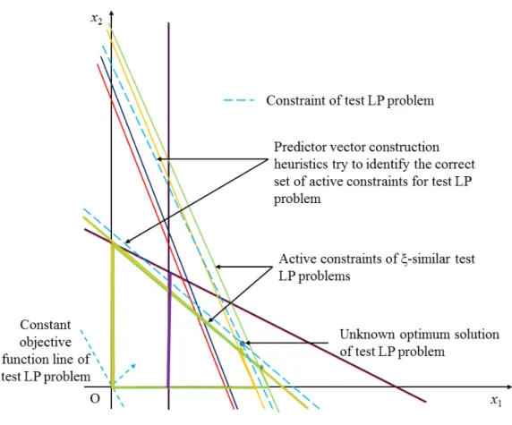
Figure 1: Schematic illustration ofξ-similar LP problems that have a common feasible region and identical optimal solutions

Let us select ξc = 0.1 and ξA = [0.1 0.1 0.1 0.1 0.1]T. Following the notation in

Definition 1, we can write c1 = [13 8]T, c2 = [14 8]T. The augmented constraint

matri-ces for LPE1 andLPE2 are equal to

 1 2 1 0 10_{5 2 0 1 20} 1 0 0 0 2  _and  1 2 1 0 10_{5 2 0 1 21} 1 0 0 0 2   _{respectively.}

We then apply (4) and (5) to get kc1−c2k2

kc1k2+kc2k2 = 0.0319,

kai,1−ai,2k2

kai,1k2+kai,2k2 = 0, i = 1, . . . ,4, and

ka5,1−a5,2k2

ka5,1k2+ka5,2k2 = 0.0218. Thus, we conclude thatLPE1 andLPE2 areξ-similar. Figure 1 shows the geometric representation ofLPE1 andLPE2, and illustrates our notion of similarity. The arrows originating from the constant objective function value lines show the directions along which the lines need to be translated so as to optimize the problems within the feasible regions. The feasible regions and optimal solutions are identical (or nearly identical in other cases) for theξ-similar LP problems, as the constraint and objective function coefficients are very close in terms of Euclidean distances. We now extend the concept ofξ-similar LP problems to first define aξ-similar LP prob-lem set and then aξ-similar LP problem space, both of which are used in the Boost-LP Learning algorithm to generate a suitable training set.

Definition 2 For a givenξand a finite collection of LP problemsLPf_{, theξ-similar LP problem set}

LPs_{is defined as a subset ofLP}f _{such that every problem∈LP}s_{has the same decision variable}

vector, andLPj1 ∈LPsisξ-similar to at least one otherLPj2 ∈LPs, j1 6=j2.

This set is represented as a collection of clusters, which are themselves sets, such that all the LP problems belonging to a cluster are pairwiseξ-similar to each other. We refer to each such cluster as aξ-similar LP problem cluster. With respect to the BAB trees of the repeated ILP problems that we want to solve efficiently, every cluster consists of the relaxed LP problems along the branches formed by imposing identical or nearly-identical constraints on parent LP problems that are them-selvesξ-similar. For example,LPE1 andLPE2 are both constructed by branching the root nodes of the respective trees by enforcing the additionalx1 = 2constraint, and are, thus, ξ-similar. The

ξ-similar LP problems can also comprise of neighboring sibling nodes, or even parent and child nodes in the nearby levels in large trees, where the variations in the constraints involving a few of the decision variables are small enough to satisfy the overall similarity criteria.

Definition 3 For a givenξ-similar LP problem setLPs_{of cardinalityN, theξ-similar LP problem}

space (Fs_{, C}s_{) is defined as a subset of<}n_{× <}n_{, where F}s _{is the union of the feasible regions}

of all the LP problems present inLPs_{, andC}s_{is given by[c1,min, c1,max]×. . .×[cn,min, cn,max].}

Here,ci denotes the i-th component of the objective function vectorc, andci,min(max) is equal to min(max){ci,1, . . . , ci,N}.LPsis then referred to as the member set of(Fs, Cs).

The union operation defines a combined feasible regionFs_{that contains the optimal solutions}

of all the member set LP problems even though portions of it may be infeasible for particular LP problems. Similarly, a combined objective function space is performed by taking the Cartesian product ofn1-dimensional spaces defined by the lower and upper bounds of the elements of thec vector.

The geometric representation of aξ-similar LP problem space is shown in Figure 2. The member space contains twoξ-similar LP problem clusters. The first cluster consists ofLPE1andLPE2. The second cluster contains two other problems,LPE3 andLPE4, with a common objective function and sets of constraints that are significantly different from the objective functions and the constraints present inLPE1 andLPE2. The optimal solutions and feasible regions vary significantly among the problems in the different clusters. This shows the usefulness of our definition, which enables us to simultaneously group LP problems that areξ-similar to each other but not to the rest in separate clusters, and yet define an overall mapping space for regression functions to operate on. We now use this concept to characterize any LP problem that need not be an element of the member set but belongs to this problem space. Such LP problems form our test cases, for which we infer solutions using the Boost-LP Inference algorithm. We use the ξ-similar LP problem clusters to aid us in obtaining near-optimal solutions for test problems by identifying only the ξ-similar member set problems that should be used in prediction.

Definition 4 Any LP problem is said to belong to aξ-similar LP problem space(Fs_{, C}s_{), if it is}

ξ-similar to all the problems in one of the clusters of the member set of(Fs_{, C}s_{), its feasible region}

has a non-empty intersection with Fs_{, and the point defined by its objective function vector lies}

insideCs_.

The condition of non-empty intersection of the feasible region of the LP problem under con-sideration withFs _{is required to exclude pathological LP problems where the feasible regions lie}

Figure 2: Schematic illustration of the member set of ξ-similar LP problem space consisting of four LP problems. LPE1 andLPE2 form oneξ-similar LP problem cluster, andLPE3 andLPE4 form the other cluster

completely outside of, but close enough to Fs_{, so that we cannot estimate any feasible solution}

based upon the existing training data even thoughξ-similarity still holds for any small non-zero value of theξ vector components. The other requirement of the location of the objective function vector insideCs_{arises due to the fact that all the components ofcare used in constructing the}

pre-dictor variable vector of the regression model (as explained in Section 3.2.1), and, hence, we cannot use outlier values to query the model to estimate a solution.

We can now begin explaining how to use a given training set ofN feasible and bounded LP problems and their optimal solutions to predict the unknown optimum solution of any arbitrary test LP problem. The training set problems are first arranged into aξ-similar LP problem setLPs_using

a minimum linkage clustering algorithm. Every problem is first considered as an individual cluster and the cluster pairs are then hierarchically merged using the minimumξ-similarity based distance (Definition 1) between any two elements in the two clusters. We discard all the problems that are not member elements of one of theξ-similar problem clusters. This clustered training set forms the member set of aξ-similar LP problem space(Fs_{, C}s_{). (Ak, bk, ck)represents the data of thek-th}

to formulate the regression problem as described in Section 3.2, and learn the boosting tree-based regression models as detailed in Section 3.3. For inference, we first verify that the test LP problem belongs to(Fs_{, C}s_{)but is not identical to any of the problems present inLP}s _{before applying a}

suitable form of the regression predictor vector and the learned boosting tree models to estimate the optimum solution.

3.2 Regression Formulation

The Boost-LP Learning algorithm outputs a set ofnregressor functions, each of which is a map-ping of the formfi : (Fs, Cs) → <, which is then used by the Boost-LP Inference algorithm to

estimate the optimumxfor any test LP problem. Each regressor function requires a predictor vari-able vector denoted byv, and a scalar response variable represented byy. Thus, we want to learn fi:v7→yi,1≤i≤n, wherevis identical for allfi, andyi =xifor everyfi. A separate regressor

function is used for inferring each component ofxto avoid the sample complexity associated with learning multiple response variables simultaneously. The inter-dependence of the decision variables is captured by incorporating the problem constraints in the predictor variable vector and by intro-ducing the penalization loss function (discussed in section 3.3). The optimum decision variable value,x∗

i, acts as the training set response variable for the corresponding functionfi.

Constructing the predictor variable vector is significantly more challenging for both training and test problems. The challenges arise from the facts that a) we only want to retain those useful problem data (constraint and objective function coefficients) that result in certain feasible solutions becoming optimal, and b) the vector is reasonably compact and its size is independent of the number of training and test LP problem constraints. We devote the rest of this sub-section to explain our construction procedure that address these challenges.

3.2.1 PREDICTORVARIABLEVECTORCONSTRUCTIONMETHOD

A na¨ıve way to generate the predictor variable vector is to include all the elements inAk, bk, and

ck following some sequence. For example, we can construct a predictor vector by concatenation

as[a1

1, . . . , a1n, b1, . . . , am1 k, . . . , anmk, bmk, c1, . . . , cn]T. This construction not only results in a very

high-dimensional vector, it can also lead to variable dimensionality for different training set prob-lems since the number of constraints,mk, may not be the same for allLPk. Adding elements to

make the dimensionality constant leads to two further issues. First, we need a systematic way of populating these elements. And, second, we cannot handle the scenario where the test problem results in a higher-dimensional vector than the one generated from the training set. Nevertheless, some pilot trials were conducted to evaluate the effectiveness of this method without considering the second issue, either by inserting zeros or random values that lie uniformly within the span of the coefficients for the additional elements. In both the cases, the regression model performed sig-nificantly worse than using thevconstruction procedure discussed below in a scheduling problem domain (described in section 5.2) with respect to both computation time and solution prediction accuracy.

Construction ofvduring learning: To construct a useful representation ofvduring the training phase (we describe how to do the same during testing afterwards), we begin from the system of constraints for thekth training set problemLPkas given by

where Ak ∈ <mk,n andbk ∈ <mk. From the underlying theory of LP problems, the optimum

solution is given by a basic feasible solution, which always exists for any feasible and bounded LP problem that is expressed in the standard form. Geometrically, every basic feasible solution represents a corner or extreme point (vertex) of the feasible region as shown in Figures 1 and 2. This property of obtaining the basic feasible solution from the system of linear equations defined by the set of active constraints1_{is henceforth referred as thesimplexproperty. Accordingly, (6) can be} partitioned as

AB,kxB+ANB,kxNB =bk

where Ak = [AB,k ANB,k], x = [xTB xTNB]T, and xB and xNB refer to the basic and

non-basic solutions, respectively. Thus, the non-basic solution consists ofmk decision variables, whereas

the non-basic solution contains the remaining(n−mk)decision variables. Since the basic solution

is obtained by setting xNB = 0and then invertingAB,k, it implies that AB,k is of full rank and

consists of a set of linearly independent active constraints. We use this property to construct a suitable representation ofv.

To do so, we first introduce a matrixEkto transform (6) to a form analogous to its left-inverse

solution2_{as represented by}

dk = (EkTAk)−1EkTbk (7)

whereEk ∈ <mk,n should be non-negative to drive every component of dk toward non-negative

values and generate feasible solutions in accordance with (3).

We choose a particular form of Ek that is given bymk rows of n-dimensional unitary

vec-tors3_{. Mathematically, we represent Ek = {eq}

1, . . . , eqmk}T andAk as {a1, . . . , amk}T, where

eacheqi ∈ <1,n is a unitary row vector andqi ∈ {1, . . . , n}, 1 ≤ i ≤ mk, denotes the position

of the unity element. Thus, Ek will be of the general form

   0 0 1 0 · · · 0 ... ... ... ... ... ... 0 1 0 0 · · · 0   . We now enforce a sequence of additional rules to ensure the invertibility of ET

kAk and identify a unique

representation ofEkthat uses the simplex property.

• Rule 1: Selectqis such thateqiaTi 6= 0 ∀i. In other words, for any given row ofEk, a unity

element is placed in a column only when the corresponding coefficient in the same row ofAkis

non-zero. This selection ensures thatET

kAkis strongly non-singular whenAkis of full rank and

mk=nas all the determinants of its principal submatrices are non-zero. However, this rule does

not lead to a unique selection ofEkor guarantee non-singularity for the general case ofmk< n.

• Rule 2: Selectqis such that no column of Ek has more than one unity element and the

corre-sponding coefficient in the same row ofAkis a basic variable at the optimum solution,x∗kthat is

known during training. In conjunction with Rule 1, this rule implies that every basic variable at x∗

kis associated with a particular constraint ofAk, referred to as therelevantconstraint.

1. Active or tight constraints are those which hold tightly, i. e. become or remain equalities for a givenx.

2. We can opt for a form analogous to the right-inverse solution; this does not affect any of our subsequent design choices or the results presented in this paper.

3. A unitary vector refers to a type of unit vector such that only one of the elements of the vector is unity and the rest are all zeros. For example,[0 0 1 0]is a 4-dimensional unitary row vector.

After enforcing Rules 1 and 2, if a column ofEkonly contains zero elements, it corresponds to

a non-basic variable atx∗

k.

• Rule 3: Eliminate all the columns from Ek that only contain zero elements. Also, eliminate

the same constraints from Ak. These elimination operations turn bothEk andAk into square

matrices of dimensionalitymk×mk, where exactly one unity element is present in every row

and column of truncatedEk.

This form of the truncatedEkmatrix occurs in the Gauss elimination method of solving a system

of linear equations and is referred as the permutation matrix Pk. It has some useful properties,

notably orthogonality and the effect of permuting the rows and columns of another matrix as a result of premultiplication and postmultiplication operations, respectively. The truncated form ofAkis the

same asAB,k, which means that the relevant constraints represent the linearly independent active

constraints atx∗

k. Transformation (7) then becomes equivalent to

dk = [dTB,k dTNB,k]T = [[(PkTAB,k)−1PkT]T 0T]Tbk (8)

wheredB,k anddNB,krepresent the basic and non-basic partitions ofdk corresponding toxB and

xNB atx∗_k. Also,dB,k = A−_B,k1 bk = x∗_B,k as formally proved below in Lemma 5. Observe that,

based on Lemma 5, we no longer need any of the rules to constructdk, and can simply enforce it to

be equal tox∗

k. However, this procedure sets the background for constructing the predictor variable

vector for the test LP problems as discussed later in this sub-section.

Lemma 5 dkis equal to the optimum solutionx∗kof any training set LP problemLPkif it is chosen

according to Rules 1-3.

Proof

Mathematically,dk = [dT_B,k dT_NB,k]T, where all the components ofdNB,k are equal to 0 by

construction, and the size ofdNB,kis(n−mk). Thus,dNB,kis identical to the non-basic optimum

solution ofLPk,x∗NB,k. Now,dB,kis given by(PkTAB,k)−1PkTbkfrom (8) and, hence, the Lemma

is proved if we can show thatdB,k is the same as the basic optimum solutionx∗_B,k. This follows as

dB,k =A−_B,k1(PkT)−1PkTbk

=A−_B,k1(P_kT)TP_kTbk from the orthogonality property of the permutation matrixPk

=A−1

B,k(PkPkT)bk

=A−1

B,k(PkPk−1)bk again from the orthogonality property ofPk

=A−_B,k1bk=x∗B,k . (9)

Finally, the common predictor variable vectorvkfor all the regressor functionsfi,1 ≤i≤ n,

in a problemLPkis formed by augmentingdkwithckas given by

vk= [d1,k, . . . , dn,k, c1,k, . . . , cn,k]T . (10)

We insertckinvk so that the regression model would not try to infer optimal solutions (response

variables) using the modeled response variables of training set LP problems with very different objective functions as compared to the test problem. Note that the size ofvkis always constant and

Generating additional training data: If the range ofdi,1 ≤i≤n, is large in the training data

set, then more problems need to be generated so that additional values of those sparsely distributed components are used in learning. We first sort all thedi,kvalues in non-decreasing order and check

whether(di,k+1−di,k),1 ≤k≤ N−1,is greater than a pre-defined thresholdζi; if yes, we add

a minimum number of problems with uniformly spaced values ofdi such that(di,k+1−di,k) ≤

ζi∀k. Henceforth, N refers to the total number of training data samples that includes both the

original and the newly added samples. To generate complete LP problems corresponding to the newly created di values, we select the average values of the two original points that violated the

threshold condition for all the components ofvexceptdi. Although this procedure directly generates

the cvector, it does not yield a solution for A and b. We handle this by selecting the A andP matrices for the lowerdivalued point, and then solving forbusing (7). Although the user-specified

vectorζhelps us in bounding the approximation errors (shown in section 4) and results in improved performance (shown in section 5.2), it can potentially lead to a large number of samples. Even otherwise, acquiring sufficient amount of training data to guarantee good quality of the estimated solutions is time-consuming. We briefly discuss this as a part of future work in section 6 since addressing it is beyond the scope of the current work.

Construction ofvduring inference: As discussed earlier during the training phase construction, the main motivation is to come up with a compact form of constant sized predictor vector v that leverages the simplex property of LP problems. This motivation led to a series of rules to identify a suitable form of the square permutation matrix P with dimensionality equal to the number of problem constraints, and consequently the number of basic solution variables. We now adopt a similar procedure to computevfor the test LP problemLPte with constraint matrixAte, constraint

vectorbte, and objective functioncte.

Since optimumx,x∗

te, and the set of basic variables atx∗te are unknown forLPte, we can apply

Rules 1 and 3 but not Rule 2. Hence, we enforce the following sequence of rules in addition to Rules 1 and 3 to computePte and the resultantdte for the test LP problem.

• Rule 2a: (Applied in place of Rule 2): Select the columns of Pte that correspond to non-zero

coefficients of the non-slack and non-surplus decision variables in the same rows of Ate as the

candidate locations of the unity elementsqis. Furthermore, selectqis such that no column ofPte

has more than one unity element.

Rules 1 and 2 imply that every row of Pte, and, as a result, every row of Ate is associated

with a unique non-slack or non-surplus decision variable. As before, the constraint associated with any decision variable is termed as a relevant constraint. While training, the relevant constraints are identical to the set of linearly independent active constraints at optimumxleading to Lemma 5, the objective here is to select the relevant constraints to be as close as possible to the active constraints atx∗

teto obtain a useful form ofdte, and correspondingly an accurate estimate ofx∗te. The selection

is based on the observation that some of the non-slack and non-surplus variables must belong to the basic solution set atx∗

te.

Depending on the number of test problem constraintsmte and the total number of non-slack

and surplus variables that satisfy Rule 1 (termed as candidate variables)nNS, two cases arise that

require differentqiselection procedures:

• Case 1: mte = nNS: Selection is straightforward here as every candidate variable can be

• Case 2: mte 6=nNS: Selection is more challenging here as we need to either exclude some

candidate variables whenmte < nNS or include some slack or surplus variables that satisfy

Rule 1 whenmte > nNS. If variables have to excluded, we select them randomly from the

list of variables that are not present in the union of the basic variables at the optimal solutions of the training LP problems that areξ-similar toLPte,LPtes. If additional variables have to be

included, we choose them randomly from the intersection of the basic variables at the optimal solutions of the problems present inLPs

te. Once the required number of candidate variables

have been excluded or included, as in the previous case, we retain all possible choices ofPte.

• Rule 4: (Applied after Rules 1-3): Partitiondte intopotentialbasic and non-basic sets asdte =

[dT

B,te dTNB,te]T, wheredB,te ∈ <mte anddNB,te∈ <n−mte. All the components ofdNB,teare

set to 0, and the constraintdB,te ≥0is imposed to ensure feasibility from (3). Compute the set

of all potentialdB,teusing the set of previously computedPteanalogous to (8) as

dB,te = (PteTAB,te)−1PteTbte .

• Rule 5: Choose a particulardtefrom the potential set obtained after applying Rules 1-4 to

mini-mize the following distance function Dte=

X

LPtr∈LP_tes

kdte−x∗trk2 (11)

wherex∗

tris the optimum solution of the training problemLPtr.

Rule 5 is based on the observation that the optimal solutions ofξ-similar problems lie close to each other inFs _{(shown in Figures 1 and 2). Thus, dte that is closest to the optimal solutions of}

problems belonging toLPs

tr is going to be equal or almost-equal tox∗te. We minimize theL2 norm

instead of aξ-similarity metric-based distance as we want to find an estimated solution that lies close tox∗

tein the Euclidean distance sense. ξ-similarity is, however, used within the distance function to

assist in identifying a suitable choice ofdte among multiple feasible options. The overall predictor

vector for the test LP problem,vte, is then constructed analogous to (10) asvte = [dTte cTte]T. All

the steps for constructingvteare stated formally in Algorithm 1.

Figure 3 depicts the geometric representation of a test LP problem that isξ-similar to the second cluster but not to the first cluster of theξ-similar LP problem space shown in Figure 2. The linearly independent active constraints that generate the optimum solution for the test problem are the per-turbed forms of the active constraints of theξ-similar training set problems. The above-mentioned rules enable us to correctly identify the active constraints as the relevant constraints, which makes didentical to the unknown optimum solution. Even though this is not necessarily true (otherwise there would not be any need for learning at all), the constructeddmostly yields feasible solutions that lie close to the optimal. The benefit of our construction procedure in obtaining low prediction error bounds is formalized in section 4 by utilizing the properties of LP problems, definitions of ξ-similarity, choice of the regression distance function, and well-known principles of linear algebra. 3.3 Boosting Tree Models

Given a procedure for transforming an LP problem into a form given by the predictor variable vector vthat permits mapping of the problem data directly to the predicted optimal values of the decision

Input: A member setLPs_{ofξ-similar LP problem space(F}s_{, C}s_{)with known optimal solutionsx}∗_and

basic solutions set atx∗_{of each of the LP problems, a test LP problemLP}

tewith data(Ate, bte, cte) that is not an element of any of the clusters ofLPs_{but belongs to(F}s_{, C}s_{), and similarity metricξ.} Output: Predictor vectorvtethat can be fed to a regression model to infer an approximately optimum

solution ofLPte.

1: InitializePte←0mte,n, wheremteandnare the number of rows and columns in the constraint matrix

Aterespectively.

2: Initialize candidate setPc_{←φand the cardinality ofP}c_,Nc_←0.

3: Identify theξ-similar LP problem cluster,LPs

te⊆LPs, forLPteby checking whetherLPteand any element of each cluster ofLPs_{areξ-similar using Definition 1. Stop as soon asξ-similarity is found} for the first time as all theξ-similar problems are included in the same cluster.

4: PopulatePc_{and using the procedures described in Case 1 and Case 2 in section 3.2.1.}

5: hmin← ∞. 6: fork= 1toNc_do 7: dk←[dTB,k dTN,k]T, wheredB,k←[(PkTAte)−1PkTbte]anddN,k←0n−mte,1. 8: ifdB,k≥0then 9: hk←PLPtr∈LPtes kdk−x ∗

trk2, wherex∗tris the optimum solution of training LP ProblemLPtr.

10: ifhk < hminthen 11: hmin←hkanddte←dk. 12: end if 13: end if 14: end for 15: Constructvte←[dTte cTte]T.

Algorithm 1: Test LP Problem Predictor Variable Vector Construction

variables, we now learn regression models for a set ofξ-similar transformed LP problems. We mod-ify the gradient boosting tree algorithm (Hastie et al., 2008) to learn a regressor function separately for every decision variable. Boosting trees are chosen as they provide adequate representational power due to the generalized additive form, have proved successful in several practical large-scale applications, and give a compact model that permits efficient querying operations. The boosting tree algorithm iteratively constructs a pre-defined number of regression trees, where each regres-sion tree performs binary partitioning of thev-space to create mutually exclusive regions at the leaf nodes. Each region models the response variable using a constant value. At every partitioning step, a particular predictor variable is chosen as the splitting variable, such that creating two child regions using a splitting variable value greedily minimizes the error in estimating the response variabley based on the currently constructed model.

The regressor function is then represented as a sum ofW binary treesT(v; Θw), each of which

is given by T(v; Θw) = J X j=1 γj,wI(v∈Rj,w)

whereΘw ={Rj,w, γj,w}encodes the data of thew-th regression tree having terminal regionsRj,w

and modeling variablesγj,w,j= 1, . . . , J. The indicator functionI is defined as

I(v∈Rj,w) =

(

1 ifv∈Rj,w,

Figure 3: Schematic illustration of identifying relevant constraints to generate a suitabledvector for predicting the optimum solution of a test LP problem that belongs to aξ-similar LP problem space whose member set comprises of the training set LP problems

The regressor functionfifor estimating the optimum value of any decision variablexiis written in

an iterative form as fi,w(v) =fi,w−1(v) +ν J X j=1 γj,wI(v∈Rj,w), w= 1, . . . , W (12)

whereν ∈(0,1)is the shrinkage parameter that controls the learning rate; the modeling variable is given by

γj,w= arg min_γ

X

vk∈Rj,w

L(yk, fi,w−1(vk) +γ); yk =x∗i,k .

Here,L(y, f(v))denotes any of the standard loss functions, such asL2 or the squared-error loss,

L1or the absolute-error loss, or the more robust Huber lossLH (Hastie et al., 2008)

LH =

(

[y−f(v)]2_{, if|y−f(v)| ≤δ,}

Further details on how to obtain the child nodes from the internal parent nodes are provided in Appendix A. The Boost-LP Inference algorithm simply selects theγ value stored in the terminal region corresponding to the location of the point defined by the predictor vector of the test LP problem as the estimated optimum value ofxi.

In the Boost-LP Learning algorithm, we restrict ourselves to modeling only the response vari-ables ofξ-similar LP problems within any terminal regionRj,w. We also consider a modified form

of the standard loss functions that heavily penalizes selection of anyγj,wvalue that lies outside the

common feasible region of all theξ-similar LP problems for which the predictor vectors v lie in Rj,w. We refer to this modified loss function as thepenalization lossLp and represent it as

Lp=L(y, f(v)) +τI(y6∈Pc). (14)

Here,τ is a very large positive number andPcis the common (intersecting) feasible region of all the

ξ-similar LP problems whosev∈Rj,w. Although this modification cannot guarantee generation of

feasible solution for any test LP problem that has a bounded feasible region, it significantly increases the possibility of doing so (shown in section 5.2).

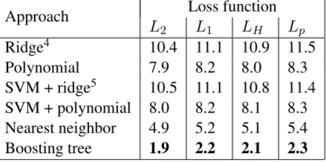
Table 1: Cross-validation error (in %) using different regression approaches.

Approach _L Loss function

2 L1 LH Lp Ridge4 _{10.4 11.1 10.9 11.5} Polynomial 7.9 8.2 8.0 8.3 SVM + ridge5 _{10.5 11.1 10.8 11.4} SVM + polynomial 8.0 8.2 8.1 8.3 Nearest neighbor 4.9 5.2 5.1 5.4 Boosting tree 1.9 2.2 2.1 2.3

Table 1 presents a comparison of the average (taken over all the response variables) cross-validation error in predicting the solutions of all the relaxed LP problems in the BAB nodes of the ILP problem instances corresponding to a repeated scheduling problem described later in sec-tion 5.2. 16 ILP problem instances are used for training, and 4 new instances are used for testing purposes. The objective function and constraint matrix remain the same in all the problem instances, and only the constraint vector differs from one instance to the other.

The ridge, polynomial (quadratic), and support vector machine (SVM) regression methods did not utilize the similarity based clustering of the training set LP problems but followed an identical predictor vector generation procedure as the boosting tree model. On the other hand, the nearest neighbor approach used a variant of the standardk-nn estimation model with equal weights given to all the neighbors, whereinkwas selected at inference time as the cardinality of the set of training LP problems that wereξ-similar to the test problem under consideration. Thus, it did not require any predictor vector construction and estimated the optimal solutions directly by averaging the optimal solutions of all theξ-similar training set problems. Since our boosting tree regression outperforms 4. Even though, strictly speaking, ridge regression uses anL2loss function, we tested all the loss functions for the sake

of consistent comparisons.L2regularization is used regardless of the loss function form.

all the other regression approaches regardless of the form of the loss function, we conclude that both similarity based clustering and generation of a compact predictor vector by leveraging the sim-plex property of LP problems are important. While using just clustering without problem structure exploitation yields better results than using problem structure without clustering, it often results in infeasible solutions as demonstrated later in section 5.1.

3.4 ILP Solution Approach

There are three salient characteristics of the Boost-LP Inference approach that uses the inferred so-lutions of the relaxed LP problems at the nodes of the BAB tree to solve the repeated ILP problem(s) which we are interested in. These characteristics are listed as follows:

• The LP solution absolute error bound (derived later in section 4.2) is added to the incumbent (current best) solution for pruning the BAB tree paths. Mathematically, it implies that we fathom any node where the estimated objective functionze_{satisfies the conditionz}e_≥z

inc+

LP, wherezinc is the current best or the incumbent solution and LP is the absolute error

bound. This a conservative pruning process that ensures that no potentially promising path, which might yield a better solution, is discarded at the cost of exploring some paths which may result in sub-optimal solutions.

• Fractional solutions are rounded off to the nearest greater or lower-valued integers if they lie within certain user-defined threshold values. Thus, ifdxe

ie −xei ≤δu, we setxei =dxeie, and

ifxe

i − bxeic ≤ δl, we setxei = bxeic, where xei is the estimated optimum value of thei-th

component of the decision variable vector. This rounding is done to account for some of the estimation errors and prevent unnecessary branching from the BAB nodes.

• Many BAB tree nodes generate infeasible or unbounded solutions for the corresponding LP problems. Since the Boost-LP algorithm cannot directly detect such cases as it has no explicit notion of any feasible region, it treats a solution as infeasible or unbounded if the correspond-ing LP problem does not belong to(Fs_{, C}s_{)or if the estimated solution satisfies the condition}

ze_{< z}e

min−LP. Here,zmine represents the estimated solution of the LP problem at the root

node, which is theoretically the minimum possible value for all the LP problems in the BAB tree. As the algorithm cannot ensure that the estimated values lie within the feasible region for problems even where feasible and bounded solutions do exist, it checks whether the estimated solution satisfies all the constraints for the problems that do not satisfy the above-mentioned conditions. If constraint violations are detected, the predicted values are discarded and the LP problem is solved using any standard optimizer.

3.5 Overall Algorithms

Algorithm tables 2 and 3 present the Boost-LP Learning and Boost-LP Inference algorithms by summarizing the various steps described earlier in this section.

4. Theoretical Results

In this section, we present an absolute performance guarantee on the test LP problem objective func-tion in the form of Theorem 12. This result is obtained by using the Cauchy-Schwarz inequality and

Input: A set ofN feasible and bounded LP problemsLPs_{, where all the problems are expressed in the} standard form and contain identical decision variables∈ <n_{, the optimal solutionsx}∗_{of all the}

problems, similarity metricξ, threshold vectorζ, Huber loss function parameterδ, number of regression treesW, number of leaf nodes in each treeJ, shrinkage parameterν, and penalization loss parameterτ. Output: A member set ofξ-similar LP problem space(Fs_{, C}s_{), a set ofnregression functions that map}

from(Fs_{, C}s_{)to<, and the LP objective function absolute error boundLP, or an error message that a} ξ-similar LP problem set cannot be created.

1: UpdateLPs_{andN by discarding the LP problems that do not form aξ-similar LP problem set} according to Definitions 1 and 2.

2: ifLPs_=φthen

3: Generate the error message and terminate.

4: else

5: Create theξ-similar LP problem space(Fs_{, C}s_{)by consideringLP}s_{as the member set using} Definition 3.

6: end if

7: fork= 1toN do

8: Generate the predictor vectorvk= [(x∗k)T cTk]T, where any problemLPk∈LPshas data

(Ak, bk, ck)and optimum solutionx∗k.

9: end for

10: fori= 1tondo 11: Sort{x∗

i,1, . . . , x∗i,N}in non-decreasing order.

12: fork= 1toN−1do 13: if(x∗

i,k+1−x∗i,k)> ζithen

14: Construct additional training set LP problems following the steps described in section 3.2.1, updateLPs_,(Fs_{, C}s_{)andNaccordingly, and constructvk for the newly-added problems.}

15: end if 16: end for 17: end for

18: fori= 1tondo 19: fork= 1toN do

20: Obtain the response variableyk =x∗i,k.

21: end for

22: Usevk, yk∀kand the parametersW,J,ν,δ, andτto generate the regression functionfithat maps from(Fs_{, C}s_{)to<following the procedure described in section 3.3. Also compute the absolute} error bound forxias given by (28).

23: end for

24: Compute the LP objective function error boundLP using (30).

Algorithm 2: Boost-LP Learning

the formula for the outer radius of the hyperbox created by boosting trees in the predictor variable vector (v) space. The hyperbox arrangement is formally stated in Lemma 8 and relies on a useful form ofvthat is specified in Lemma 5. The dimensions of the box are bounded by the prediction errors for the individual decision variables. This error is derived in Lemma 11 and depends on whether the variable is labeled as basic or non-basic. The error terms have four components. The first component is obtained in Lemma 10 based upon our choice ofvthat uses Rule 5. The second component represents the error introduced in predicting the test LP problem solution by using ξ-similar (not identical) training set LP problems, again using our particular form ofvbased on Rules 1-4; it is specified in Lemma 9. The third component depends on the complexity of the boosting tree

Input: A member set ofξ-similar LP problem space(Fs_{, C}s_{), a set ofnregression functions that map} from(Fs_{, C}s_{)to<, the LP objective function absolute error bound}

LP, similarity metricξ, threshold parameters for rounding off fractional valuesδuandδl, and a repeated ILP problem with unknown optimum solution that has not been used to generate the member set.

Output: An approximate solution of the given ILP problem.

1: Follow the BAB algorithm to construct a tree, where each node represents a relaxed LP version of the given ILP problem, branch from existing nodes to create child nodes, and fathom nodes when the paths are guaranteed to not yield any solution that is better than the incumbent.

2: Instead of solving any of the relaxed LP problems optimally using a standard solver, set the estimated solution vectorxe

te ←φand estimated objective functionztee ← −∞.

3: whileze

te=−∞do

4: ifLPtedoes not belong to(Fs, Cs)from Definition 4then

5: ze_{← ∞.}

6: else

7: Construct the predictor variable vectorvtefor the corresponding LP problemLPtewith data

(Ate, bte, cte)using Algorithm 1 and the similarity metricξ.

8: fori= 1tondo

9: Use the regression functionfiandvteto infer an approximate solutionxei,te.

10: end for 11: ze

te←cTtexete.

12: end if 13: end while

14: Use the characteristics described in section 3.4 and the input parametersLP,δu, andδlto modify the bounding step in the BAB algorithm, make certain fractional values integers, and handle infeasiblity of estimated solutions for feasible and bounded LP problems.

Algorithm 3: Boost-LP Inference

model and the last component is the user-specified vectorζthat is discussed in section 3.2. Both of these are used in Lemma 11. We begin by defining and presenting the formula for outer radius of a hyperbox.

Definition 6 Theouterj-radiusRjof ap-dimensional convex polytopePis defined as the radius of

the smallestj-dimensional ball containing the projection ofP onto all thej-dimensional subspaces, whereby the value ofRjis obtained by minimizing over all the subspaces. Note thatRpis the usual

outer radius or circumradius.

Remark 7 LetBbe ap-dimensional box (orp-box) in Euclidean spaceEp_{with dimensions2r1×}

2r2×. . .×2rp, such that{x∈Ep| −ri ≤xi ≤ri, i= 1, . . . , p}. It can be assumed without any

loss of generality that0< r1 ≤r2≤. . .≤rp. ThenRj is simply given by Brandenberg (2005) as

Rj =

q

r2

1+. . .+rj2 . (15)

4.1 Relations between Predictor Variable Vectors and Optimal Solutions

We first present a lemma that formalizes the hyperbox arrangement generated by boosting trees. This is used in deriving the performance guarantees for the test LP problem decision variables and objective function in Lemma 11 and Theorem 12 respectively.

Lemma 8 Boosting trees transform the LP problems present in the training data set to an arrange-ment ofp-dimensional, axis-aligned boxes.

Proof We have

0≤dk<∞,1≤k≤N (16)

whereN is the training data set size. The LHS inequality in (16) follows from Lemma 5 and (3), while the RHS inequality is obtained from Lemma 5 and the fact that the decision variables cannot assume infinite values that result in unbounded LP solutions (from (1)). Thus, the irregularly-shaped convex polytopes that represent the feasible regions of the LP problems are transformed into axis-aligned boxes in the completely positive2n_{-ant of then-dimensionald-space.}

The predictor variable vectorvof the boosting tree also includes the components of the objec-tive function vectorc. As both the minimum and maximum values ofci must be finite∀i(infinite

values again lead to unbounded LP solution as given by (1)),cforms another axis-aligned box of dimensionalityn. Thus, the overallvspace is also a boxB of higher dimensionalityp= 2n. Since each node in a regressor tree is formed by performing binary partitioning of thevspace, every ter-minal tree region corresponds to ap-dimensional boxB0 _{⊆B, thereby creating an arrangement of} boxes.

We now present a lemma that provides an upper bound on the absolute difference between any component of the dvector of the test LP problem and the optimum value of the corresponding decision variable of aξ-similar LP problem that belongs to the training data set. This result is used Lemma 11 to derive the performance bounds for the test problem decision variables.

Lemma 9 Aξ-similar training LP problem (LPtr) exists for any test LP problem (LPte) such that

the maximum value ofdi,te−x∗_i,tr,1 ≤ i ≤ n, is bounded by a constant that depends on the

similarity vectorξA, the data of the training set LP problems, and whetherxi,tr andxi,teare basic

or non-basic.

Proof

LPte must be ξ-similar to at least one of the training set LP problems, as otherwise it does

not belong to theξ-similar LP problem space whose member set is given by the training set (from Definition 4), and, hence, is not regarded as a test problem at all. Let us denote that ξ-similar training problem byLPtr6. From (5), using the propertykai,te−ai,trk2 ≥ |kai,tek2− kai,trk2|, we

have

|kai,tek2− kai,trk2|

kai,tek2+kai,trk2 ≤ξi,A .

Therefore, ifkai,tek2≥ kai,trk2, we get

kai,tek2− kai,trk2 ≤ξi,A(kai,tek2+kai,trk2)

⇒kai,tek2(1−ξi,A)≤ kai,trk2(1 +ξi,A)

⇒_kka_ai,tek2

i,trk2 ≤

1 +ξi,A

Alternatively, ifkai,tek2 <kai,trk2, we have k_ka_ai,tri,tek_k2₂ ≥ _ξi,r1 . Asξi,ris always greater than 1 (since

ξi,A ∈ (0,1]in Definition 1), (17) holds true regardless of whetherkai,tek2 is greater than or less

thankai,trk2.

We can then re-write (17) as

X j (aj_i,te)2 _≤ξ2 i,r X j (aj_i,tr)2 =X j (aj_i,tr+i,tr)2 (18)

wherei,tris a small number that is given by one of the solutions of the quadratic equationP_j(aj_i,tr+

i,tr)2−ξi,r2 Pj(aji,tr)2 = 0(see Appendix B for greater details). Now, (18) is satisfied ifaji,te ≤

aj_i,tr+i,tr∀i, j. So, by selectingtr = max{1,tr, . . . , n,tr}and a non-negative matrixF ∈ <mte,n

suitably with no element greater than 1, we get

Ate =Atr+trF (19)

where only the matched set of constraints are considered inAtr when mtr > mte. By replacing

thei-th column ofAteandAtrwithbteandbtr, and denoting the resulting matrices byAiteandAitr

respectively, we have an analogous expression given by

Ai_te =Ai_tr+i_trFi (20)

wherei

tr = max{1,tr, . . . , i−1,tr, n+1,tr, i+1,tr. . . , n,tr}. Note that (19) and (20) are also valid

for truncated forms of the constraint matrices that only contain the columns corresponding to the basic solutions.

The deviation betweendi,teandx∗_i,trcan be decomposed into four different cases: first, when the

corresponding decision variable in bothdi,te andx∗i,tr is either selected by the Rules in section 3.2

or known to be a basic variable, second, when the decision variable is considered to be basic inLPte

but is actually non-basic inLPtr, third, when the decision variable is considered to be non-basic in

LPte but is actually basic inLPtr, and fourth, when the decision variable is non-basic in bothLPte

andLPtr. The absolute deviation is exactly given byx∗i,trin the third case asdi,teis equal to 0, and

by 0 in the last case as bothdi,te andx∗_i,tr are equal to 0. Let us now derive the expressions for the

first two cases.

For the first case, we have

_di,te−x∗ i,tr= det(Ai H,te) det(AH,te) −x ∗ i,tr

from Cramer’s rule (21)

whereAH,te denotes the rule-determined truncatedA matrix ofLPte that gives the non-zero

(ex-pected to be basic at optimum x∗

te) components of dte. Combining (21) with (19) and (20), we

get _di,te−x∗ i,tr= det(Ai H,tr+itrFHi) det(AH,tr+trFH) −x ∗ i,tr