Turbulence Modeling Verification and Validation (Invited)
Christopher L. Rumsey
∗NASA Langley Research Center, Hampton, VA 23681-2199
Turbulence modeling for the Reynolds-averaged Navier-Stokes (RANS) equations includes many assump-tions and simplifying closures. Numerous models have been developed over the years, and all are deficient in one way or another. Many collective efforts have attempted to validate turbulence models for a wide range of problems, but conclusions have often been muddied due to the lack of grid convergence, lack of model verifi-cation in different codes, or for other reasons. In this paper, turbulence modeling verifiverifi-cation and validation is discussed primarily within the context of several recent workshops. A web-based turbulence modeling resource is also described, whose goals include turbulence model documentation, verification, and validation. Using this resource, specific models can easily be put through a verification testing procedure, helping to eliminate coding errors.
I.
Introduction
Computational fluid dynamics (CFD) software that solves the Reynolds-averaged Navier-Stokes (RANS) equations has been in routine use for more than a quarter of a century. It is currently employed not only for basic research in fluid dynamics, but also for the analysis and design processes in many industries worldwide, including aerospace, automotive, power generation, chemical manufacturing, polymer processing, and petroleum exploration.1
A key feature of RANS CFD is the turbulence model. Because the RANS equations are unclosed, a model is necessary to describe the effects of the turbulence on the mean flow, through the Reynolds stress terms. The turbulence model is one of the largest sources of uncertainty in RANS CFD, and most models are known to be flawed in one way or another. Alternative methods such as direct numerical simulations (DNS) and large eddy simulations (LES) rely less on modeling and hence include more physics than RANS. In DNS all turbulent scales are resolved, and in LES the large scales are resolved and the effects of the smallest turbulence scales are modeled. However, both DNS and LES are too expensive for most routine industrial usage on today’s computers. Hybrid RANS-LES, which blends RANS near walls with LES away from walls, helps to moderate the cost while still retaining some of the scale-resolving capability of LES, but for some applications it can still be too expensive.
Even considering its associated uncertainties, RANS turbulence modeling has proved to be very useful for a wide variety of applications. For example, in the aerospace field, many RANS models are considered to be reliable for computing attached flows. However, existing turbulence models are known to be inaccurate for many flows involving separation. Research has been ongoing for decades in an attempt to improve turbulence models for separated and other nonequilibrium flows.
When developing or improving turbulence models, both verification and validation are important steps in the process. Verification insures that the CFD code is solving the equations as intended (no errors in the implementation). This is typically done either through the method of manufactured solutions (MMS)2 or through careful step-by-step comparisons with other verified codes. After the verification step is concluded, validation is performed to document the ability of the turbulence model to represent different types of flow physics. Validation can involve a large number of test case comparisons with experiments, theory, or DNS.
Organized workshops have proved to be valuable resources for the turbulence modeling community in its pursuit of turbulence modeling verification and validation. Workshop contributors using different CFD codes run the same cases, often according to strict guidelines, and compare results. Through these comparisons, it is often possible to (1) identify codes that have likely implementation errors, and (2) gain insight into the capabilities and shortcomings of different turbulence models to predict the flow physics associated with particular types of flows. These are valuable lessons because they help bring consistency to CFD codes by encouraging the correction of faulty programming and
∗Senior Research Scientist, Computational AeroSciences Branch, Mail Stop 128, Fellow AIAA.
facilitating the adoption of better models. They also sometimes point to specific areas needed for improvement in the models.
In this paper, several recent workshops are summarized primarily from the point of view of turbulence modeling verification and validation. Furthermore, the NASA Langley Turbulence Modeling Resource websiteais described. The purpose of this site is to provide a central location where RANS turbulence models are documented, and test cases, grids, and data are provided. The goal of this paper is to provide an abbreviated survey of turbulence modeling verification and validation efforts, summarize some of the outcomes, and give some ideas for future endeavors in this area.
II.
Workshops
Over the years, there have been numerous workshops focused either all or in part on turbulence modeling veri-fication or validation. Below, several workshops and workshop series familiar to the author are highlighted. Taken together, these have helped to identify strengths and weaknesses of turbulence models for particular problems of interest. They have also highlighted difficulties that occur when attempting to compare results from different codes.
A. ERCOFTAC SIG 15 Workshops on Refined Turbulence Modeling
The European Research Community on Flow, Turbulence, and Combustion (ERCOFTAC) has sponsored a series of workshops since 1991 on “Refined Turbulence Modeling.” These have been part of its special interest group number 15 (SIG15) on turbulence modeling. The workshops have focused on a wide variety of different test cases through the years, over a series of 14 workshops. The last workshop was held in 2009. Some of the cases included separated flow over a hill, swirling boundary layer in a conical diffuser, wing-body junction with separation, 2-D plane wall jet, flow around a cube, rotating plane channel flow, axisymmetric plane diffuser flow, flow around a simplified car shape, flow over an axisymmetric 3-D hill, flow in a 3-D diffuser, and jets in crossflow.
In the more recent SIG15 workshops, the turbulence modeling focus has shifted from primarily RANS modeling to include more scale-resolving methods such as hybrid RANS-LES, LES, and DNS. However, here only a brief summary of some of the major RANS-related conclusions from the workshops will be mentioned. Only those workshops whose results were summarized in the documentation provided on the ERCOFTAC websitebare covered here.
In the 4th ERCOFTAC SIG15 workshop3from 1995, one of the cases involved 2-D hill flows. For this, mostk-ε
models tended to predict the separation zone too small, whilek-ωmodels tended to predict it too long. However, all models—including full second-moment Reynolds shear stress models (RSM)—underpredicted the level of turbulent kinetic energy and turbulent shear stress in the separated shear layer. For a swirling boundary layer in a conical diffuser, standardk-ε models with wall functions were reasonable (apart from insufficient reduction in center-line velocity); more advanced models offered little improvement. In a curved rectangular duct, explicit algebraic stress models (EASM) and RSMs seemed to yield closer agreement than simpler models. However, for this case as well as others, it was difficult to reach a general conclusion due to inconsistencies between results obtained with nominally the same turbulence model. For example, for the curved rectangular duct, three different calculations with the same standardk-εmodel with wall functions displayed large differences between them.
In the 5th ERCOFTAC SIG15 workshop4 from 1996, the same curved rectangular duct case was used from the
previous workshop. Simplek-εmodels tended to yield poor results. EASMs and RSMs performed generally better (particularly concerning the secondary flow details), but not for all aspects. For example, RSMs performed no bet-ter than linear eddy viscosity models in predicting the asymmetry of the kinetic energy profile from the inner wall (where the curvature has a damping effect) to the outer wall (where the curvature has an enhancing effect). Again the same model in different codes produced different results, making firm conclusions difficult. Grid resolution varied considerably between participants, and appeared to have a big impact.
The 9th ERCOFTAC SIG15 workshop5was held in 2001. The four cases were: swirling flow, periodic 2-D hill
flow, perturbed backward-facing step flow, and flow over a simplified car body. For the swirling flow, previous uncer-tainties from the experiment were mitigated by including LES computations. Nonetheless, this flow was concluded to be “not especially challenging” for turbulence models. The 2-D hill flow, similar to one from the earlier workshop, proved very challenging for models. Again, models under-predicted the turbulent shear stress in the recirculation zone (mixing was too weak in the shear layer bordering the separation bubble). For the backstep, the computations did not capture the rate of increase in turbulent shear stress due to imposed perturbations. Finally, for the car body, seven
aRumsey, C. L., http://turbmodels.larc.nasa.gov, accessed 10/22/2013.
groups obtained very different results, even with the same turbulence models. This inconsistency—attributed to insuf-ficient grid resolution, lack of convergence, and coding errors—made it difficult to draw conclusions. Pessimistically, it was concluded that “keeping in mind the experience from the previous workshops, it will probably never be possible to achieve fully consistent solutions by using the same model schemes.” This paper will return to a discussion of this subject in Section IV.
The 10th workshop6 in 2002 used the same hill and car body cases, along with a new contra-rotating jet case.
For the hill, based on LES it was emphasized that large scale low frequency unsteadiness near the separation and reattachment points make this case challenging for statistical methods such as RANS, which cannot predict its mean effect. The turbulent shear stress and turbulent kinetic energy were under-predicted as usual in the separated shear layer, and separation bubble length was typically predicted too long. Some models (notably lineark-ε) yielded more reasonable bubble sizes and broadly correct velocity profiles, but this was fortuitous. These models had a tendency to predict late separation, resulting in earlier reattachment for the wrong reasons.7 RANS models also again did poorly
for the car body, for unknown reasons. For the contra-rotating jet, it was clear that linear eddy-viscosity turbulence models were not well-suited. However, even nonlinear models such as RSMs were unable to reproduce the transition from wake to mixing layer behavior.
At the 11th workshop8in 2005, the CFDVAL2004 wall-mounted hump with and without flow control (see CFD-VAL2004 section below) was included in an attempt to elicit additional conclusions beyond those reached at the original CFDVAL2004 workshop. However, results were generally similar. A 3-D hill flow, 3-D slanted jets in cross-flow, and 3-D multiple impinging jet flow all proved to be very difficult for RANS; no major conclusions were reached other than “3-D fields are still very difficult to compute.” For the slanted jets it was noted that two implementations of the samek-ωmodel yielded different results: one predicted a pair of focal points downstream of the injector as seen in the experiment, the other did not.
The 12th workshop9in 2006 again included the wall-mounted hump and 3-D hill, plus a tip-gap flow and a swirl
combustor. Nothing new was learned for the first two cases, and the other cases were only computed by one group each. The attendance at this workshop was among the lowest of all the SIG15 workshops to date. The reason for the low participation was believed to be the difficulty in computing the 3-D cases, and the growing belief that only scale-resolving methods such as hybrid RANS/LES or LES could be successful for the more difficult cases.
The 13th workshop10 was held in 2008. The first case was a round jet impinging on a rotating heated disc. Eddy
viscosity RANS models were able to capture some effects, but missed details such as redistribution among turbulent stress components. RSMs performed better in this regard, as expected. The second case was a 3-D separated diffuser, for which both RANS and scale-resolving methods were applied. RANS eddy viscosity models were all similarly poor. Only a single EASM result returned the correct flow topology.
Finally, the 14th workshop11in 2009 focused on the same 3-D separated diffuser. Greater emphasis was placed on scale-resolving methods at this workshop. From the RANS results, it was learned that an important prerequisite for success was capturing the strong secondary flow in the inlet region. This is not possible with linear RANS models. Among nonlinear models, both EASM and RSM methods were capable of predicting flow topology in reasonable agreement with experiment (with some differences). Near-wall treatment was felt to be “not of decisive importance.” Differing grid resolutions and inadequate grid refinement studies were felt to be at least partly to blame for many of the disagreements between results.
Overall, the ERCOFTAC series of turbulence modeling workshops have been very instructive. They have high-lighted (1) cases for which simple RANS turbulence models work reasonably well, (2) cases for which only nonlinear models such as EASM or RSM work, and (3) cases for which RANS in any form fails. The series has also pointed out the importance of adequate grid refinement, and the difficulty in getting different codes with ostensibly the same turbulence model to agree. This latter issue has been a primary cause for the difficulty in drawing firm conclusions.
B. Workshops on CFD Uncertainty Analysis
A series of three verification workshops12–14was held in Lisbon in 2004, 2006, and 2008. The focus of this series was somewhat different from the ERCOFTAC series, dealing in large part with the evaluation of uncertainty estimators such as the grid convergence index (GCI).15However, verification and validation also played a large role. At the first workshop, a 2-D hill and 2-D backward facing step were investigated. Unfortunately, doubt was engendered because of “conceptual modeling differences and the possibility of undetected coding errors.” The modeling differences included boundary condition inconsistencies between participants. In some cases the inconsistencies came about because some codes could not handle all boundary condition types.
The second workshop sought to overcome these issues through the specification of analytical solutions prescribed by MMS, which mimicked 2-D turbulent near-wall flow. This proved to be a very useful exercise, in some cases
leading participants to discover errors in their codes. It was also learned that the order of accuracy of the turbulent transport equations can influence the observed order of accuracy of the mean flow quantities. This is of interest because in current practice many CFD codes use first-order discretization for the turbulence convection terms. This practice may degrade the mean flow convergence to first order in the limit of very fine grid sizes. It was also found that the observed order of accuracy of a given turbulence model did not always match the theoretical order expected. However, Eca et al. noted that “the analyses for theoretical order are neither obvious nor unique for highly nonlinear problems” such as for those involving RANS turbulence models. A physical problem of a backward facing step was attempted, but there was a general failure to achieve sufficient grid resolution (i.e., the calculations were not on fine enough grids to lie in the asymptotic range of convergence).
The third workshop included (1) verification via MMS, (2) verification for the backward facing step problem, and (3) validation for the backward facing step problem, including both CFD and experimental uncertainty estimates. Most participants included the Spalart-Allmaras (SA) turbulence model.16 An interesting outcome was the fact that
SA submissions for the backward facing step became more consistent over the course of the three workshops. In part, this improved consistency may have been a result of participants finding coding mistakes when using MMS. See Figs. 1(a) - (d). In these figures, taken from Eca et al.,14SA results of four different measures for the backward facing step are plotted from three different workshops. The first workshop results are on the right side of each figure, second workshop is in the middle, and third workshop is on the left. The figures show friction resistance coefficient on the top wall, friction resistance coefficient on the bottom wall, pressure resistance coefficient on the bottom wall, and reattachment point, respectively. Estimated uncertainty for each submission is included as error bars. Ignoring four of the submissions in the 2008 workshop (submissions 1, 2, 6, and 7), the remaining ten SA results were in extremely close agreement. Notably, the four submissions with different results were from commercial software codes. One of these used much coarser grids than the other participants, and the other did not perform the code verification exercise and was believed to have a coding error in its implementation of SA.
Other conclusions from the third workshop included the fact that RANS solvers do not always converge with the theoretical order of accuracy of the schemes adopted in the discretization of the equations. The reasons for this inconsistency were not determined. Furthermore, demonstrating that a data set lies within the asymptotic range can be very difficult. For one thing, different flow quantities of the same solution may behave differently (one may lie in the asymptotic range and the other may not). For another, use of only a single evaluation of the observed order of accuracy was found to be unreliable. Because of this, one may need to either apply an increased factor of safety to the error estimate, or else perform more work with additional grids in order to better estimate the observed order of accuracy.
Follow-ups to this workshop series were conducted in different settings and formats after 2009, but these are not discussed here.
C. CFDVAL2004
The CFDVAL2004 workshop held in 2004 focused on validation of synthetic jets and turbulent separation control.17 Three cases were considered: (1) nominally 2-D synthetic jet into quiescent air, (2) circular synthetic jet in a crossflow, and (3) 2-D flow over a wall-mounted hump. Case 3 included a baseline no-flow-control condition, a steady suction condition, and an oscillatory synthetic jet condition, all three of which featured a separation bubble. The summary of the CFDVAL2004 workshop noted that CFD variation was quite large, possibly in part due to inconsistent application of boundary conditions. It was suggested that future experiments focus on documenting the time-dependent boundary conditions at and near the exit plane of the jet or suction slot or orifice. It was also noted that there did not appear to be obvious benefits from using high-order numerical methods for these cases. In other words, the deficiencies from turbulence modeling far outweighed any benefits from improved numerical accuracy.
Detailed results for each of the three test cases can be found in Rumsey et al.17Only a few highlights are described
here. Case 1 was problematic in that the flow was likely not fully turbulent, and became three-dimensional beyond a certain distance above the jet slot. Case 2 appeared to be more sensitive to grid, code, and other solution variations than to turbulence model choice. Participants obtained reasonably good qualitative results overall, in spite of an unexplained large cross-flow velocity during the expulsion part of the cycle in the experiment that was not modeled in any of the CFD. The case 3 hump experiment was felt to be the most reliable and well-documented of the three cases. It provided very clear evidence for RANS model deficiencies. Case 3 was very similar to the hill cases considered in the ERCOFTAC workshop series, and indeed—like the ERCOFTAC hill cases—RANS models yielded poor results at this workshop as well, producing too little turbulent shear stress in the shear layer above the bubble, and consequently tending to reattach the bubble too late. Fig. 2(a) demonstrates how most workshop participants predicted a separation bubble longer than experiment for the steady suction control in case 3. Note that the RANS indicated separated flow at a location where the experimental results were already reattached. Results were similarly poor for the case with
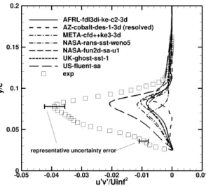
no flow control. Typical RANS underprediction of turbulent shear stress in the bubble region is shown in Fig. 2(b). Most participants’ models produced peaku0v0 magnitude about a factor of 3 or 4 too small. Interestingly, even scale-resolving methods did not agree well with experiment at the original workshop (more on this below).
After the 2004 workshop, there were over 16 CFD papers written on case 1, 7 CFD papers written on case 2, and 44 CFD papers on case 3. An important aspect of the success and longevity of this workshop’s impact is the fact that the experimental data, CFD results, grids, and other documentation were posted to a publicly-available websitec,
which was assiduously maintained for many years following the workshop itself. This allowed other researchers to easily take up and investigate these cases.
In fact, some improvements were made in CFD simulations for these cases over subsequent years, particularly through improved boundary condition usage and through the use of scale-resolving simulations. These improvements have been summarized elsewhere.18 Specifically for the wall-mounted hump (case 3), it was noted that no major
progress was made since the time of the workshop in terms of RANS. Results have for the most part been very consistent in terms of predicting too little eddy viscosity in the separated region and too long a bubble. It was noted that models can sometimes predict a particular feature like reattachment location correctly for the wrong reasons. For example, becausek-εturbulence models tend to predict smooth-body separation caused by adverse pressure gradient too late, they also tend to predict earlier reattachment. This reattachment location may appear to agree better with experiment in the hump case, for example, but it is not due to better modeling of the turbulent mixing in the separated region; i.e., thek-εphysics are still wrong.
Post-workshop computations using scale-resolving hybrid RANS-LES, LES, and “coarse-grid DNS” improved significantly, in most cases obtaining significantly better results than RANS. Much of the scale-resolving CFD im-provements came about because of improved grid resolution. By resolving (in space and time) many of the 3-D turbulent eddies in the flow field, the mixing due to turbulence in separated regions was better predicted. Fig. 3 shows bubble reattachment locations from the workshop, with subsequent improved results superimposed using filled-in symbols. In this figure, the best results for both cases were from LES. Detached eddy simulation (DES),19 a hybrid
RANS-LES method, performed well for the no-flow-control case, but it had trouble predicting the small separation bubble for the suction case. Coarse-grid DNS result showed marked improvement by doubling the grid resolution (“double grid” in the figure), indicating that further grid refinement is likely required for this method. The computa-tional requirements for scale-resolving methods can be quite high, e.g., hundreds of millions of grid points (or more) and on the order of a hundred thousand time steps for the DNS. This is in contrast to perhaps hundreds of thousands of grid points and ten thousand time steps for typical highly-resolved 2-D RANS (i.e., on the order of104less compute resources for RANS than for DNS).
The CFDVAL2004 workshop helped to clarify and highlight both practical issues such as boundary condition usage for flows that employ flow control, as well as particular failings of RANS turbulence models applied to separated flows both with and without flow control. Providing easy web-based access to the data, grids, and other pertinent information was instrumental in giving the cases broad appeal. Although to date RANS methods have undergone no significant improvement for computing hump-type separated flows, scale-resolving results have improved largely due to greater computer capabilities and more user experience with these methods. Whether RANS models can be improved for separated flows (possibly with the help of data from high-quality LES or DNS simulations) remains to be seen.
D. DPW and HiLiftPW series
The Drag Prediction Workshop (DPW) and High Lift Prediction Workshop (HiLiftPW) series, sponsored by the AIAA Applied Aerodynamics Technical Committee, have been very well-attended since their respective inceptions. To date there have been five DPWs and two HiLiftPWs. One of the most appealing aspects of these workshops is that they provide publicly-available configurations and grids with associated experimental data for industry-relevant configu-rations. DPW’s primary focus is prediction of forces and moment for transport aircraft geometries in cruise config-uration, whereas HiLiftPW’s primary focus is similar prediction in high-lift configuration (i.e., with flaps and slats deployed).
Here, only a few observations and trends are noted related to turbulence modeling for these workshops. More details can be found elsewhere.20–25Overall, no clear trends have been established regarding the best RANS turbulence model to use for these configurations. Most participants have favored the use of the Spalart-Allmaras (SA)16or Menter shear-stress transport (SST) model26or their variant. These two models have been well-tested in industrial codes over
the last 20 years and their capabilities and limitations are fairly well known. They are also generally very robust and easy to run. The SA and SST models are implemented in many different CFD codes, so it would be reasonable to
expect that results for each of these models should be consistent when run on a given case by different CFD codes. However, this has generallynotproven to be the case for DPW and HiLiftPW.
Throughout much of the DPW series, the presence of separated regions (particularly in the wing-root junction with the fuselage) has been a source of much of the differences exhibited between participant results. However, the predicted separation bubble size has not been solely a function of turbulence model, as might be expected. It also appears to be very strongly a function of grid and numerical method. In DPW-5, the organizers required participants to run on a provided set of grids. This helped reduce CFD scatter from earlier workshops for the cruise case (no separation). But at higher angle-of-attack, significant variation was still observed, partly because of different results for side-of-body separation. Some studies have been performed by workshop participants regarding the side-of-body separation issue. For example, Sclafani et al.27 showed that the bubble size increased with grid refinement, and solving
the thin-layer form of the RANS equations yielded a smaller bubble than the full form of the equations. Yamamoto et al.28 also showed the bubble size to be strongly influenced by grid size, topology, and numerical dissipation. They
further demonstrated that use of SA with a quadratic constitutive relation (QCR)29as opposed to a linear eddy viscosity
relation helped to significantly reduce the size of the bubble predicted.
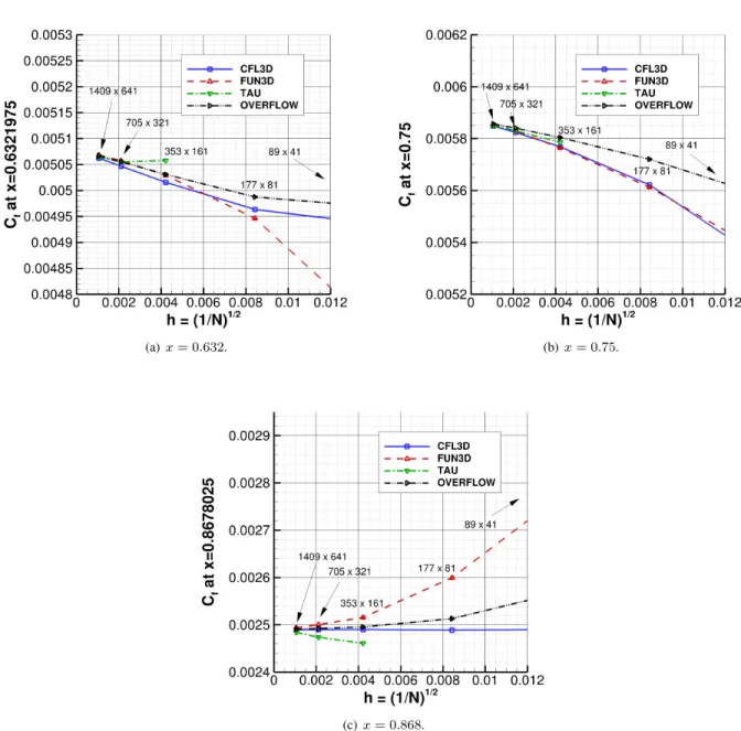
In order to try to get a handle on reasons for inconsistencies between different codes using the same turbulence model, DPW-5 and HiLiftPW-2 also included a turbulence model verification study, motivated by the on-line NASA Turbulence Modeling Resource (see next section). In DPW-5, use of simple well-defined test cases along with grid convergence studies uncovered potential differences in turbulence modeling implementations. Because the verification cases were so simple, it was easier to identify specific problems. For example, the 2-D bump verification case helped to isolate differences due to incorrect or inaccurate computation of the minimum distance function,d, which is used in both the SA and SST models. Fig. 4 shows grid convergence behavior at a specific location on the bump. At the DPW-5 workshop, only contributions denoted as T4, T10, and T11 agreed with each other as the grid was refined. After discussion, it was discovered that T2, T5, and T6 had used an inaccurate method for calculating d. Their predicted skin friction coefficient on the finest grid was high by over 3%. These participants subsequently corrected their computations, resulting in near-perfect agreement with the others, as shown in the figure. (The reason for the contributions T1 and T3 disagreeing was not discovered.) It is important to perform this type of verification study as a first step and try to resolve all issues prior to tackling more difficult configurations.
Although not shown here, the verification study further demonstrated that small but quantifiable differences can be expected between two commonly used forms of the SST model. In one (standard SST), the turbulence production is computed using turbulent stress along with mean strain terms; in the other (SST-V), an approximate production term based on turbulent stress and mean vorticity terms is employed instead. Many times in workshops, the two methods are used by participants interchangeably, with no distinction made between them. Experience has shown that it is better to indicate specifically which version is used, both for repeatability sake as well as to help discern possible reasons for differences between results.
To date, there have been two HiLiftPWs held. Although not discussed here, the second workshop, which computed flow over a DLR-F11 configuration, is summarized in Rumsey and Slotnick.30 A summary of the first workshop,
which used the NASA Trapezoidal Wing configuration, can be found in Rumsey et al.25 In terms of turbulence
modeling, most participants of HiLiftPW-1 favored SA or SST. A few other models includingk-ω,k-ε, and RSM were also used. SA tended to yield higher lift than other models, in better agreement with experiment, while the SST model (for example) tended to predict too much separation on the flap. However, it was noted that transition could play a significant role for this case (Reynolds number based on mean aerodynamic chord was 4.3 million). Several participants31–33subsequently demonstrated that a transition-enabled version of the SST model (γ-Re
θSST)34
performed much better than SST run fully turbulent. Eliasson et al.35 demonstrated similar improvements for the SA
model using aneN transition method. In other words, the use of fully-turbulent simulations for high-lift cases like these may miss important transitional physics that can significantly impact results. An example showing the influence of including transition for the Trapezoidal Wing is shown in Fig. 5. Results using SST produced a large region of separated flow over the flap atα= 13◦, whereas theγ-Re
θSST model yielded significantly less separation and 4%
higher lift, in better agreement with experiment.
It should be noted that HiLiftPW-1 also included the complication of hysteresis. In the NASA Trapezoidal Wing experiments, hysteresis was evident both beyondCL,maxas well as at very low angles of attack near zero. In the CFD,
some of the workshop participants noted that at higher angles of attack it was necessary to use initial conditions from converged lower angles of attack in order to avoid massive separation. Kamenetskiy et al.36 subsequently performed
a study of multiple solutions for RANS on high lift configurations. The appearance of multiple solutions seemed to be closely related to smooth body separation, particularly evident near stall angles of attack. They believed that spurious solutions could be identified and dismissed if they changed drastically with grid refinement, adaptation, or
small perturbations.
Much time and effort has been spent during the DPW and HiLiftPW series trying to discern the reasons for the (at times) large variations between participant results. Certainly it seems to be within our capability today to insure that the CFD codes employed have at least implemented the turbulence modelsas intended, without significant coding errors or intentional undocumented fixes. Verification exercises can help in this regard (see next section). Attention can then turn to other issues such as grid resolution, numerics, geometric and boundary condition fidelity, transition, and iterative convergence.
III.
Turbulence Modeling Resource Website
The NASA Langley Research Center Turbulence Modeling Resource Website was established in the late 2000’s in an effort to help improve the consistency, verification, and validation of turbulence models within the aerospace community. This grew in part in response to an assessment37 from a turbulence modeling workshop held in 2001.
One of the major conclusions from that workshop was that “a national/international database and standards for turbu-lence modeling assessment should be established.” Later, a working group of the AIAA called the Turbuturbu-lence Model Benchmarking Working Group (TMBWG) was established with a similar goal. This website is now guided by the TMBWG. Additional details can be found on the website itself, or in related papers.38, 39Since its inception, the web-site has grown considerably, although its scope remains the same. Its main objective is to provide a resource for CFD developers to (1) obtain accurate and up-to-date information on widely-used RANS turbulence models, and (2) verify that models are implemented correctly.
The website is divided into several distinct sections. The first, “Turbulence Models,” lists specific turbulence models, including many of their known variants. Naming conventions have been established in order to help avoid confusion when comparing results from different codes. As of the time of this writing, 11 different turbulence model categories are described. It is hoped that turbulence modelers will be motivated to help include new model ideas to the site, in order to speed dissemination into the aerospace community.
The second section, “Turbulence Model Verification Cases and Grids,” provides four different simple cases that can be useful for helping to verify model implementation. For each case, a large sequence of nested grids of the same family are provided, along with results from existing CFD codes that employ specific forms of particular turbulence models (currently only SA, SST, SST-V, and Wilcox200640 are available). Example grid convergence study results
for the 2-D bump case using SST are shown in Fig. 6. Surface skin friction levels at three locations on the bump are compared on successively finer grids. Four different CFD codes are shown to approach approximately the same result ash→0. With four different independent codes yielding the same grid-refined results, other model implementers can be very confident that this is the result that SSTshouldobtain for this case, when coded correctly. With the grids and other relevant data provided, it is a relatively simple matter for anyone in the world to test their implementations of the currently-available models.
The third section, “Turbulence Model Validation Cases and Grids,” provides a variety of simple validation cases, including wall-bounded, shear, and jet flows. These cases are intended to give the reader a feel for the capabilities and limitations of various models when applied to different classes of simple problems. This section of the website undergoes the most revisions and additions, as new test cases or model results are added. It should be noted here that each turbulence model tested in the Validation section is assigned what is referred to as a Model Readiness Rating (MRR) number. In essence, this number indicates how widely tested the model is. A new model that is described and referenceable, but not necessarily coded, is assigned level 0. If in addition the model is in at least one CFD code and has been run on the flat plate case with grid study (and results made available), it is assigned level 1. Level 2 is for a model in two or more CFD codes whose results agree; the model must also have been run on two or more verification/validation cases. Finally, level 3 is achieved when the model is implemented in independent codes from different organizations and results have been independently obtained and verified.
The fourth section, “Turbulent Flow Validation Databases,” contains potentially useful data from experiments, DNS, and LES. Some of the experimental databases are from earlier work collated by Peter Bradshaw, who for many years was very actively engaged to validate and improve turbulence models.41 The fifth section, “Turbulent Manu-factured Solutions,” provides information from the Lisbon Workshops on CFD Uncertainty Analysis (described in an earlier section). Manufactured solutions and associated Fortran subroutines for several different turbulence models are included. The sixth (relatively new) section is on “Cases and Grids for Turbulence Model Numerical Analysis.” Here, cases designed primarily for numerical analysis of turbulence model simulations are presented. In other words, the focus is mainly on issues such as turbulence model convergence properties, effects of order of accuracy, etc.
location for finding the equations that describe turbulence models themselves (including their variants). It also con-tains grids and data to help CFD researchers to verify their implementations of models. This is made possible by demonstrating grid convergence behavior of multiple codes, all of which approach the same answer. Although not as rigorous as methods such as MMS, this method of verification is simpler and is surprisingly effective at highlighting problems due to coding or implementation errors. It is certainly an easy first step to take in the verification process. Finally, by providing data from various sources, this website also helps in the turbulence model validation process.
IV.
Summary and Recommendations
Turbulence modeling has always been the Achilles heel of RANS CFD. All models are inherently flawed, which makes them easy scapegoats when CFD results do not agree with experiment. There are, however, many other possible sources of error, including grid resolution, numerics, geometric and boundary condition fidelity, transition, iterative convergence, and coding/implementation errors. As described in this paper, many workshops in recent years have sought to evaluate the capabilities and highlight the flaws of existing turbulence models for a wide variety of problems. By doing this, new model improvements may be motivated. Unfortunately, too often workshop results have been muddied by the fact that different CFD codes with ostensibly the same model have obtained very different results for unknown reasons.
For many years it was considered nearly impossible to insure consistency between different codes, but recent ef-forts have sought to ameliorate this problem by making it easier for researchers to verify their implementations of turbulence models. Turbulent manufactured solutions for a variety of different specific turbulence models are avail-able, although their use requires some additional coding. The NASA Langley Research Center Turbulence Modeling Resource Website also provides a simplified verification process for several widely-used models, which requires no additional coding and has proven to be very effective. A sensible recommendation for future workshops would be to follow the idea espoused in the Lisbon workshop series, and require evidence of model verification prior to perform-ing validation studies. This would help prevent codperform-ing/implementation errors from obscurperform-ing the conclusions. Also, the importance of websites for broadcasting workshop data, grids, and results as widely as possible cannot be over-emphasized. The easier such information is to obtain (before, during, and after the workshop), the more researchers will take it up, increasing the possibility of future improvements or breakthroughs.
As computer capability continues to improve and we move toward the next CFD era dominated by scale-resolving simulations, these more accurate methods offer promise to play a part in improving RANS turbulence models. More workshops should strive to include high-quality DNS and LES simulations of canonical cases, designed to highlight particular physical features for which state-of-the-art turbulence models are known to be lacking. Because of the wealth of data that they can provide, these high-quality simulations may be used to access quantities of interest to turbulence modelers that are difficult to measure in experiments.
For the foreseeable future, RANS will remain an important tool in the analysis and design of many engineering fluid flow processes. Methodical research should continue in this important area, with the goal of improving turbulence model capabilities for wider classes of problems. In addition, continued workshops that focus on both verification and validation will help bring together the research community to tackle common CFD goals and improve the state-of-the-art.
References
1Davidson, D. L., “The Role of Computational Fluid Dynamics in Process Industries,”The Bridge, National Academy of Engineering, Vol. 32, No. 4, Winter 2002, pp. 9–13.
2Roy, C. J., Nelson, C. C., Smith, T. M., and Ober, C. C., “Verification of Euler/NavierStokes Codes Using the Method of Manufactured Solutions,”International Journal for Numerical Methods in Fluids, Vol. 44, 2004, pp. 599-620.
3Bonnin, J. Ch., Buchal, T., and Rodi, W., “ERCOFTAC Workshop on Data Bases and Testing of Calculation Methods for Turbulent Flows,” (Karlsruhe, Germany), ERCOFTAC Bulletin, No. 28, 1996, pp. 48–54.
4Laurence, D., “5th ERCOFTAC Workshop on Refined Flow Modelling for Turbulent Flows,” (Chatou, France), ERCOFTAC Bulletin, No. 33, 1997, pp. 10–13.
5Jakirlic, S., Jester-Zurker, R., and Tropea, C., “9th ERCOFTAC/IAHR/COST Workshop on Refined Turbulence Modelling,” (Darmstadt, Germany), ERCOFTAC Bulletin, No. 55, 2002, page numbers not known.
6Manceau, R., “Report on the 10th Joint ERCOFTAC (SIG-15)/IAHR/QNET-CFD Workshop on Refined Turbulence Modelling,” (Poitiers, France), ERCOFTAC Bulletin, No. 57, 2003, page numbers not known.
7Leschziner, M. A., “Test Case 9.2: The Flow in a Channel with Periodic Hills on One Wall,” Proceedings of the 10th Joint ERCOFTAC (SIG-15)/IAHR/QNET-CFD Workshop on Refined Turbulence Modelling, October 10-11, 2002, CNRS Universite de Poitiers, Poitiers, France, Eds: R. Manceau, J.-P. Bonnet, M. A. Leschziner, F. Menter.
8Johansson, T. G. and Davidson, L., “11th ERCOFTAC Workshop on Refined Turbulence Modelling,” (Goteborg, Sweden), ERCOFTAC Bulletin, No. 69, 2006, page numbers not known.
9Thiele, F. and Jakirlic, S., “12th ERCOFTAC/IAHR/COST Workshop on Refined Turbulence Modelling,” (Berlin, Germany), ERCOFTAC Bulletin, No. 75, 2007, page numbers not known.
10Steiner, H., Jakirlic, S., Kadavelil, G., Manceau, R., Saric, S., and Brenn, G., “13th ERCOFTAC Workshop on Refined Turbulence Mod-elling,” (Graz, Austria), ERCOFTAC Bulletin, No. 79, 2009, pp. 22–27.
11Jakirlic, S., Kadavelil, G., Sirbubalo, S., von Terzi, D., Breuer, M., and Borello, D., “SIG15 Workshop on Refined Turbulence Modelling,” (La Sapienza, Italy), ERCOFTAC Bulletin, No. 85, 2010, pp. 5–13.
12Eca, L., Hoekstra, M., and Roache, P. J., “Verification of Calculations: an Overview of the Lisbon Workshop,” AIAA Paper 2005-4728, June 2005.
13Eca, L., Hoekstra, M., and Roache, P. J., “Verification of Calculations: Overview of the 2nd Lisbon Workshop,” AIAA Paper 2007-4089, June 2007.
14Eca, L., Hoekstra, M., and Roache, P. J., “Code Verification, Solution Verification and Validation: an Overview of the 3rd Lisbon Workshop,” AIAA Paper 2009-3647, June 2009.
15Roache P. J.,Verification and Validation in Computational Science and Engineering, Hermosa Publishers, Albuquerque, New Mexico, 1998. 16Spalart, P. R. and Allmaras, S. R., “A One-Equation Turbulence Model for Aerodynamic Flows,”Recherche Aerospatiale, No. 1, 1994, pp. 5–21.
17Rumsey, C. L., Gatski, T. B., Sellers, W. L. III, Vatsa, V. N., and Viken, S. A., “Summary of the 2004 Computational Fluid Dynamics Validation Workshop on Synthetic Jets,”AIAA Journal, Vol. 44, No. 2, 2006, pp. 194–207.
18Rumsey, C. L., “Successes and Challenges for Flow Control Simulations,”International Journal of Flow Control, Vol. 1, No. 1, 2009, pp. 1–27.
19Spalart, P. R., Jou, W.-H., Strelets, M., and Allmaras, S. R., “Comments on the Feasibility of LES for Wings, and on a Hybrid RANS/LES Approach,”Advances in DNS/LES, 1st AFOSR International Conference on DNS/LES, edited by C. Liu and Z. Liu, Greyden Press, Columbus, 1997, pp. 137–148.
20Levy, D. W., Zickuhr, T., Vassberg, J., Agrawal, S., Wahls, R. A., Pirzadeh, S., and Hemsch, M. J., “Data Summary from the First AIAA Computational Fluid Dynamics Drag Prediction Workshop,”Journal of Aircraft, Vol. 40, No. 5, 2003, pp. 875–882.
21Laflin, K. R., Vassberg, J. C., Wahls, R. A., Morrison, J. H., Brodersen, O., Rakowitz, M., Tinoco, E. N., and Godard, J., “Summary of Data from the Second AIAA CFD Drag Prediction Workshop,”Journal of Aircraft, Vol. 42, No. 5, 2005, pp. 1165–1178.
22Vassberg, J. C., Tinoco, E. N., Mani, M., Brodersen, O. P., Eisfeld, B., Wahls, R. A., Morrison, J. H., Zickuhr, T., Laflin, K. R., and Mavriplis, D. J., “Abridged Summary of the Third AIAA CFD Drag Prediction Workshop,”Journal of Aircraft, Vol. 45, No. 3, 2008, pp. 781–798.
23Vassberg, J., Tinoco, E., Mani, M., Rider, B., Zickuhr, T., Levy, D., Broderson, O., Eisfeld, B., Crippa, S., Wahls, R., Morrison, J., Mavriplis, D., and Murayama, M., “Summary of the Fourth AIAA CFD Drag Prediction Workshop,” AIAA Paper 2010-4547, June 2010.
24Levy, D., Laflin, K., Tinoco, E., Vassberg, J., Mani, M., Rider, B., Rumsey, C., Wahls, R., Morrison, J., Broderson, O., Crippa, S., Mavriplis, D., and Murayama, M., “Summary of Data from the Fifth AIAA CFD Drag Prediction Workshop,” AIAA Paper 2013-0046, January 2013.
25Rumsey, C. L., Slotnick, J. P., Long, M., Stuever, R. A., and Wayman, T. R., “Summary of the First AIAA CFD High-Lift Prediction Workshop,”Journal of Aircraft, Vol. 48, No. 6, 2011, pp. 2068–2079.
26Menter, F. R., “Two-Equation Eddy-Viscosity Turbulence Models for Engineering Applications,”AIAA Journal, Vol. 32, No. 8, 1994, pp. 1598–1605.
27Sclafani, A. J., DeHaan, M. A., Vassberg, J. C., Rumsey, C. L., and Pulliam, T. H., “Drag Prediction for the NASA CRM Wing-Body-Tail Using CFL3D and OVERFLOW on an Overset Mesh,” AIAA Paper 2010-4219, June-July 2010.
28Yamamoto, K., Tanaka, K., and Murayama, M., “Comparison Study of Drag Prediction for the 4th CFD Drag Prediction Workshop using Structured and Unstructured Mesh Methods,” AIAA Paper 2010-4222, June-July 2010.
29Spalart, P. R., “Strategies for Turbulence Modelling and Simulation,”International Journal of Heat and Fluid Flow, Vol. 21, 2000, pp. 252-263.
30Rumsey, C. L. and Slotnick, J. P., “Overview and Summary of the Second AIAA High Lift Prediction Workshop (Invited),” AIAA Paper to appear, January 2014.
31Steed, R. G. F., “High Lift CFD Simulations with an SST-Based Predictive Laminar to Turbulent Transition Model,” AIAA Paper 2011-0864, January 2011.
32Sclafani, A. J., Slotnick, J. P., Vassberg, J. C., and Pulliam, T. H., “Extended OVERFLOW Analysis of the NASA Trap Wing Wind Tunnel Model,” AIAA Paper 2012-2919, June 2012.
33Rumsey, C. L. and Lee-Rausch, E. M., “NASA Trapezoidal Wing Computations Including Transition and Advanced Turbulence Modeling,” AIAA Paper 2012-2843, June 2012.
34Langtry, R. B. and Menter, F. R., “Correlation-Based Transition Modeling for Unstructured Parallelized Computational Fluid Dynamics Codes,”AIAA Journal, Vol. 47, No. 12, 2009, pp. 2894–2906.
35Eliasson, P., Hanifi, A., and Peng, S.-H., “Influence of Transition on High-Lift Prediction for the NASA Trap Wing Model,” AIAA Paper 2011-3009, June 2011.
36Kamenetskiy, D. S., Bussoletti, J. E., Hilmes, C. L., Venkatakrishnan, V., Wigton, L. B., and Johnson, F. T., “Numerical Evidence of Multiple Solutions for the Reynolds-Averaged Navier-Stokes Equations for High-Lift Configurations,” AIAA Paper 2013-0663, January 2013.
37Rubinstein, R., Rumsey, C. L., Salas, M. D., and Thomas, J. L., “Turbulence Modeling Workshop,” NASA/CR-2001-210841, March 2001; also ICASE Interim Report no. 37, 2001.
38Rumsey, C. L., Smith, B. R., and Huang, G. P., “Description of a Website Resource for Turbulence Modeling Verification and Validation,” AIAA Paper 2010-4742, June-July 2010.
39Rumsey, C. L., “Consistency, Verification, and Validation of Turbulence Models for Reynolds-Averaged Navier-Stokes Applications,”
Jour-nal of Aerospace Engineering, Proc. IMechE Part G, Vol. 224, 2010, pp. 1211–1218.
41Bradshaw, P., Launder, B. E., and Lumley, J. L., “Collaborative Testing of Turbulence Models,”Journal of Fluids Engineering, Vol. 118, June 1996, pp. 243–247.
(a) Top wall friction resistance coefficient (b) Bottom wall friction resistance coefficient
(c) Bottom wall pressure resistance coefficient (d) Reattachment point
Figure 1. Backward facing step results using the SA model from three Lisbon uncertainty workshops (figure from Eca et al.,14used with permission).
(a) U-velocity profiles downstream of the experimental bubble reattach-ment location
(b) Turbulent shear stress across separation bubble
Figure 2. Example results from CFDVAL2004 wall-mounted hump suction case, from Rumsey et al.17
(a) No flow control (b) Suction flow control
Figure 3. Hump model reattachment locations from original workshop along with more recent DES, LES, and DNS results (filled-in symbols), from Rumsey.18
Figure 4. Convergence verification study on 2-D bump using SA model from DPW-5, showing six independent entries reaching the same grid-converged result, and effect of inaccurated.
(a) Upper surface streamlines, SST model (fully turbulent), com-putedCL= 1.9848.
(b) Upper surface streamlines,γ-Reθ SST transitional model, computedCL= 2.0581.
Figure 5. Effect of transition on upper surface streamlines for HiLiftPW-1 case atα = 13◦(CL,exp = 2.0474), from Rumsey and
(a)x= 0.632. (b)x= 0.75.
(c)x= 0.868.
Figure 6. Grid convergence of skin friction coefficient for four independent codes on 2-D bump case using the SST model, from the NASA Langley Turbulence Modeling Resource website.