An Inverse-Gamma Source Variance Prior with Factorized Parameterization for Audio Source Separation

An Inverse-Gamma Source Variance Prior with

Factorized Parameterization for Audio Source

Separation

Dionyssos Kounades-Bastian, Laurent Girin, Xavier Alameda-Pineda, Sharon

Gannot, Radu Horaud

To cite this version:

Dionyssos Kounades-Bastian, Laurent Girin, Xavier Alameda-Pineda, Sharon Gannot, Radu

Horaud. An Inverse-Gamma Source Variance Prior with Factorized Parameterization for Audio

Source Separation. International Conference on Acoustics, Speech and SIgnal Processing, Mar

2016, Shanghai, China. pp.136-140,

<

10.1109/ICASSP.2016.7471652

>

.

<

hal-01253169

>

HAL Id: hal-01253169

https://hal.inria.fr/hal-01253169

Submitted on 8 Jan 2016

HAL

is a multi-disciplinary open access

archive for the deposit and dissemination of

sci-entific research documents, whether they are

pub-lished or not.

The documents may come from

teaching and research institutions in France or

abroad, or from public or private research centers.

L’archive ouverte pluridisciplinaire

HAL

, est

destin´

ee au d´

epˆ

ot et `

a la diffusion de documents

scientifiques de niveau recherche, publi´

es ou non,

´

emanant des ´

etablissements d’enseignement et de

recherche fran¸

cais ou ´

etrangers, des laboratoires

publics ou priv´

es.

AN INVERSE-GAMMA SOURCE VARIANCE PRIOR WITH FACTORIZED

PARAMETERIZATION FOR AUDIO SOURCE SEPARATION

Dionyssos Kounades-Bastian

, Laurent Girin

, Xavier Alameda-Pineda

, Sharon Gannot

, Radu Horaud

_{INRIA Grenoble Rhˆone-Alpes,}

_{GIPSA-Lab, Univ. Grenoble Alpes}

3

_{University of Trento,}

_{Faculty of Engineering, Bar-Ilan University}

ABSTRACT

In this paper we present a new statistical model for the power spectral density (PSD) of an audio signal and its application to multichannel audio source separation (MASS). The source signal is modeled with the local Gaussian model (LGM) and we propose to model its variance with an inverse-Gamma distribution, whose scale parameter is factorized as a rank-1 model. We discuss the interest of this approach and evaluate it in a MASS task with underdetermined convolutive mixtures. For this aim, we derive a variational EM algorithm for param-eter estimation and source inference. The proposed model shows a benefit in source separation performance compared to a state-of-the-art LGM NMF-based technique.

Index Terms— Audio modeling, local Gaussian model, PSD model, audio source separation.

1. INTRODUCTION

For the past decade, the statistical modeling of audio signals in the time-frequency (TF) domain has been thoroughly in-vestigated. Among the proposed models, the local Gaussian model (LGM) [1] has become very popular because, among other reasons, it can be naturally coupled with models of the signal power spectral density (PSD) (which identifies with the signal variance at each TF bin for a zero-mean signal). An important example is the use of non-negative matrix factor-ization (NMF), which imposes a low-rank structure on the PSD matrix, namely the product of a spectral pattern ma-trix and a temporal activation mama-trix [2]. Intuitively, NMF is meant to efficiently represent the structure of the audio sig-nal power in the TF domain with a reduced number of pa-rameters. The NMF factors were first treated as parameters [3, 4, 5, 2], and then as latent variables within a Bayesian framework [6, 2, 7, 8, 9].

These models have been successfully applied to audio source separation. In MASS configurations, the source signal models are combined with a mixing model, accounting for the source-to-sensor channels, e.g. [10, 11, 12, 13, 14]. In general, an EM algorithm is derived to estimate the source

This research has received funding from the EU-FP7 STREP project EARS (#609465) and ERC Advanced Grant VHIA (#340113).

and channel parameters, which are then used to construct demixing Wiener filters. Besides, a general framework for inserting prior information about the sources in TF-domain MASS has been proposed in [15].

In current Bayesian NMF PSD models, the source PSD is first modeled with NMF and, second, the NMF factors are assigned a prior distribution. In this paper, we propose to change the order of things: The source is still seen as a sum of components, but we first assign a prior distribution to the component PSD and then assume a factorized model, reminis-cent of NMF, on the parameters of this distribution. More pre-cisely, we model the component PSD with an inverse-Gamma (IG) distribution and assume that the scale parameter of this IG follows a rank-1 NMF. As explained in Section 2, this en-ables to add flexibility in the modeling of source PSD matrix, compared to conventional NMF, while preserving the abil-ity to model structured source PSD. We apply the proposed model to MASS from underdetermined convolutive mixtures. The proposed model is presented in Section 2. The as-sociated variational EM (VEM) algorithm that we derived to estimate the model parameters and infer the source signals is described in Section 3. Experimental evaluation reported in Section 4 shows competitive performances in comparison to the state-of-the-art LGM-NMF MASS method of [10].

2. MODELS 2.1. The mixing model

As usually done in the MASS literature, we work under the narrow-band assumption, which allows us to write a time-invariant convolutive mixture in the short-term Fourier trans-form (STFT) domain as:

xf `=Afsf `+bf `, (1) wherexf ` = [x1,f `, . . . , xI,f `]> ∈ CI is theIchannel

ob-servation vector,sf `= [s1,f `, . . . , sJ,f `]>∈CJis the source

vector to be inferred, Af ∈ _CI×J _{is a mixing matrix}

pa-rameter to be estimated, andbf ` ∈ CI is the sensor noise.

We assume p(bf `) = Nc(bf `;0,vfII),1 with vf ∈ R+

1_N

c(x;µ,Σ) =|πΣ|−1exp −[x−µ]HΣ−1[x−µ]is the proper complex Gaussian distribution withx∈CI,µ∈CIandΣ∈CI×I.

being a variance parameter to be estimated (II is the iden-tity matrix of dimensionI). The above assumption implies

p(xf `|sf `) = Nc(xf `;Afsf `,vfII). Note that the above

mixture can be underdetermined, i.e. we can haveI < J.

2.2. The source model

We embrace the LGM framework [1, 10] wheresj,f ` ∈ C

is assumed to follow a zero-mean proper complex Gaussian distribution. Moreover,sj,f `is assumed to be the sum of

ele-mentary componentsck,f ` ∈C, also zero-mean proper

com-plex Gaussian:

sj,f ` =

X

k∈Kj

ck,f `⇔sf `=Gcf `, (2)

whereKj is a subset of a nontrivial partitionK ={Kj}Jj=1

(known in advance) of theKcomponents into theJ sources,

cf ` = [c1,f `, . . . , cK,f `]> ∈ CK is the vector of component

coefficients, andG∈ NJ×K is a binary matrix with entries

Gjk = 1ifk ∈ Kj andGjk = 0otherwise. Finally, as in

[10], we assume that all{ck,f `}F,L,K<sub>f,`,k=1</sub>are independent, with:

p(ck,f `|uk,f `) =Nc(ck,f `; 0, uk,f `). (3)

In particular, the source PSD at each TF bin is the sum of individual component PSDs at that bin.

2.3. The component PSD model

Traditionally, the component PSD (or component variance)

uk,f ` is typically assumed to factorise overf and`, i.e. an

NMF model is applied on the source PSD directly. In a Bayesian framework, the NMF factors are assigned a prior distribution. The main contribution of this paper is to reverse the traditional order: We first assume a prior distribution for the component variance and then impose a nonnegative factorized structure on its parameters. More precisely, we assume that each entryuk,f ` of the component PSD matrix

follows an inverse Gamma (IG) distribution2_:

p(uk,f `) =IG(uk,f `;γk, δk,f `) withδk,f `=wf khk`, (4)

whereγk, wf k, hk` ∈ R+. The choice for the IG

distribu-tion emerges naturally, as it is the conjugate prior of the vari-ance of a Gaussian. The factorization of the scale parameter

δk,f `into a rank-1 model is a key point of our model. Indeed,

modeling theparametersof the component PSD prior (for in-stanceδk,f `) with a rank-1 model instead of the component

PSDuk,f `itself allows the latter not to be constrained to have

a low-rank structure. Therefore, with the proposed model, both the component PSD and the source PSD can be full-rank,

2_{The Inverse Gamma distribution is defined as IG(u;γ, δ) =} (δ)γ

Γ(γ)u

−(γ+1)_exp−δ u

, with supportu ∈ R+, shape parameterγ ∈

R+, scale parameterδ∈R+, andΓ(·)being the Gamma function.

uk,f `

γk, wf k, hk` ck,f ` xf ` vf,Af

Fig. 1. Graphical reprsentation of the probabilisitc model. La-tent variables are represented with circles, observations with double circles, deterministic parameters with rectangles.

as opposed to conventional NMF. In the meantime, the pro-posed model keeps a limited number of parameters and an ability to represent structured signals, in the spirit of conven-tional NMF. Finally, we postulate that the proposed model has the potential to better represent natural audio signals, such as speech. As for the IG shape parameterγk, it intuitively acts as

a measure of the relevance of thek-th component: high (resp. low) values ofγkdecrease (resp. increase) the contribution of

thek-th component.

3. VARIATIONAL INFERENCE

We propose an EM algorithm to perform inference of the hid-den variablesH={cf `, uk,f `}

F,L,K

f,`,k=1 and estimation of the

parametersθ={Af,vf, γk, wf k, hk`} F,L,K

f,`,k=1. As the E-step

does not admit a closed form solution, we use variational in-ference: Letq(H0) =p H0|{xf `}F,L<sub>f,`=1</sub>;θdenote the poste-rior distribution of a variableH0∈ H. Firstq(H)is imposed to factorise as q(H) ≈ QF,L f,`=1q(cf `) QF,L,K f,`,k=1q(uk,f `). Thenq(H0) =p(H0| {xf `} F,L f,`=1;θ)is infered with: q(H0)∝expEq(H/H0) logp(H,{xf `}<sub>f,`</sub>F,L₌₁;θ), (5) whereEq(z)[f(z)]is the expectation of functionalf(z)w.r.t.

the distributionq(z)over the support of the variablez, and whereq(H/H0)is the joint posterior distribution of all hid-den variables exceptH0. The resulting E-step is the alternat-ing inference ofq(cf `)(E-C), andq(uk,f `)(E-U),∀f, `, k.

3.1. E-step

Let the superscript(r)denote the (V)EM iteration index, i.e.

θ(r)are the parameters computed at therthiteration.

E-U-step: First we consider the inference ofq(uk,f `).

Using (5), one can easily identifyq(uk,f `)to be also an IG:

q(uk,f `)∝p(uk,f `) exp Eq(cf `)[logp(ck,f `|uk,f `)] =IGuk,f `;g (r) k , d (r) k,f ` , (6)

with posterior parametersg_k(r), d(_{k,f `}r) ∈R+calculated as:

g_k(r)=γ_k(r−1)+1, d(_{k,f `</sub>r) =δ<sub>k,f `}(r−1)+ Σ<sub>kk,f `</sub>c(r−1)+cˆ (r−1) k,f ` 2 , (7) whereΣc_{kk,f `}(r−1)∈R+is thekthdiagonal entry ofΣ

c(r−1)

f ` , and

ˆ

c(<sub>k,f `</sub>r−1) ∈ Cis thekth entry ofˆc(f `r−1), both being calculated

E-C-step: Using (5), q(cf `) can be identified to be complex-Gaussian: q(cf `)∝p(xf `|Gcf `) K Y k=1 exp Eq(uk,f `)[logp(ck,f `|uk,f `)] =Nc cf `; ˆc (r) f `,Σ c(r) f ` . (8)

The posterior covariance matrixΣc_{f `}(r)∈_CK×K_and

compo-nent vector estimateˆc(_{f `}r)∈CKare given by:

Σc_{f `</sub>(r)=   diagK g<sub>k</sub>(r−1) d(<sub>k,f `}r−1) ! + A(_fr−1)G H A(_fr−1)G v(_fr−1)    −1 , ˆ c_{f `</sub>(r)=Σ<sub>f `}c(r)A(_fr−1)G H xf `/v(_fr−1), (9) where diag_K(xk)is theK×Kdiagonal matrix with entries

x1, . . . , xK. Eq. (9) corresponds to the Wiener filtering of

the component, thus a similar result as in [10] except for the construction of the component posterior covariance matrix.

Estimating the source coefficients:Now, using (2), it is easy to calculate the source posterior distribution, which as one expects, is a complex Gaussian with meanˆs(_{f `}r) ∈ CJ,

and2nd_{-order momentR}s(r)

f ` ∈C J×J<sub>calculated as:</sub> ˆs(<sub>f `</sub>r)=Gˆc_{f `</sub>(r), Rs<sub>f `}(r)=GΣc_{f `</sub>(r)G>+ ˆs<sub>f `}(r)ˆs(_{f `}r) H . (10) 3.2. M-step

As for the M step, the parameters maximizing the expected complete-data log-likelihood are computed.

M-Af step: The optimal value for the filters is:

A(_fr)= 1 L L X `=1 xf `ˆs(<sub>f `</sub>r) H! <sub>1</sub> L L X `=1 Rs_{f `}(r) !−1 , (11)

which is a standard form of least square estimator [10].

M-vfstep: The optimal noise variance is:

v(_fr)= 1 LI L X `=1 xHf `xf `−2Re n xHf `A (r) f ˆs (r) f ` o + tr Rs<sub>f `</sub>(r)A(_fr) H A(_fr) ! , (12)

where tr{.}is the trace operator.

M-IG step: The IG parameters(γk, wf k, hk`)are

cou-pled in the objective function and thus an alternating opti-mization strategy is required, i.e. fixing two parameters to estimate the third. The updates forwf k, hk`are:

w(_{f k}r)= Lγ (r−1) k g(_kr) L P `=1 h(<sub>k`</sub>r−1) d(_{k,f `</sub>r) , h(<sub>k`}r)= F γ (r−1) k g(_kr) F P f=1 w(_{f k}r−1) d(_{k,f `}r) . (13)

Algorithm 1Separation ofJstatic sound sources

input{xf `} F,L

f,`=1, binary matrixG, initial parametersθ (0)<sub>.</sub> initialiseIG parameters:ng<sub>k</sub>(0), d(0)<sub>k,f `</sub>o

F,L,K

f,`,k=1,setr= 1. repeat

E-C step: ComputeΣc_{f `</sub>(r) andˆc(<sub>f `}r)with (9). Compute

ˆs(_{f `</sub>r)andRs<sub>f `}(r)with (10).

E-U step: Calculateg_k(r)andd(_{k,f `}r) , with (7).

M-Afstep: UpdateA (r) f with (11). M-vf step: Update v (r) f with (12).

M-IG step: Update w_{f k}(r), h(_k`r) with (13). Calculate

δ_{k,f `</sub>(r) =w(<sub>f k</sub>r)h(<sub>k`}r). Updateγ_k(r)with (15).

setr=r+ 1.

untilconvergence

return the estimated source images.

Then we setδ_{k,f `</sub>(r) =w<sub>f k</sub>(r)h(<sub>k`}r), and the update forγ_k(r)is the solution w.r.tγ_k(r)to: ψg(_kr)−ψγ_k(r)= 1 F L F X f=1 L X `=1 log d (r) k,f ` δ(_{k,f `}r) ! , (14)

where ψ(.) is the digamma function. Since (14) has no closed-form solution, we propose to approximate g(_kr) with

γ(_kr)+ 1, relying on (7), and use the recurrence relation of the digamma functionψ(x+ 1) =ψ(x) + 1_x. This leads to the following update rule:

γ_k(r)= 1 1 F L F P f=1 L P `=1 log d(<sub>k,f `</sub>r) δ(_{k,f `}r) . (15)

3.3. Estimation of source images

Considering the inherent scale indeterminacy of the source separation problem, we rather measure the separation per-formance using the (time domain) source images, i.e. the estimates of the source signals as recorded at the micro-phones [11, 16]. These are calculated by applying inverse STFT with overlap-add on{aj,fsˆj,f `}F,Lf,`=1 (aj,f is thej-th

column ofAf). The complete VEM procedure can be found in Algorithm 1.

4. EXPERIMENTS

To asses the performance of the proposed algorithm, we simulated the challenging task of separatingJ = 3sources from a convolutive stereo mixture (I = 2). Source signals were 2s-speech signals randomly chosen from the TIMIT database [17]. As mixing filters, we used binaural room

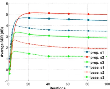
Fig. 2. Average SDR score as a function of (V)EM iterations (Mix-1,R= 0dB).

impulse responses (BRIR) from [18] truncated to 512 taps with reverberation time of RT60 ≈ 0.68s. Two sets of

BRIRs were used, corresponding respectively to azimuths

−85◦,−20◦,60◦ (Mix-1), and azimuths −45◦,75◦,10◦

(Mix-2). Standard sound separation measures, namely signal-to-distortion ratio (SDR) and signal-to-interference-ratio (SIR) [19] were computed. All reported results are average measures over8sets of utterances (for each mix).

To ensure a fair comparison with the baseline method [10], we provided both algorithms with the same initial informa-tion. The mixing filters were blindly initialized toA(0)_f =1(a matrix filled with ones) and we set v(0)_f = _{F LI}103 P

f `(xf `)

H_{xf `,}

∀f. As for the NMF parameters, each source was cor-rupted with the sum of the two other sources at two different SNRs (R = 10dB or 0dB). An initial NMF decomposi-tion{winit

f k , h init

k` }f,`,kwas then computed for each corrupted

source PSD using the KL-NMF algorithm [2], with|Kj|= 20

components per source. {winit

f k , hinitk` }f,`,kwere also used to

initialize the NMF parameters of the baseline method. We setδ(0)<sub>k,f `</sub> = winit f k h init k` , γ (1) k = 1andd (0) k,f ` = δ (0) k,f ` (thus g(0)_k = 2andE_IG(u k,f `;g(0)k ,d (0) k,f `) [uk,f `] = winitf k hinitk` ). We run 100 iterations.

Fig. 2 shows the average SDR obtained at each iteration for Mix-1 withR = 0dB. We observe a quite regular evolu-tion of the SDR scores, which are quite stabilized after 100 it-erations (after some possible decrease, since the (V)EM does not guarantee monotonic evolution of the separation scores as opposed to the likelihood). For this mix, the proposed method shows a notable improvement over the baseline: up to 3.1dB fors2 (remind that these scores are averaged over 8

experi-ments with same filters but different sources). Final perfor-mance (at iteration 100) for other configurations, and for SIR

Table 1. Average SDR and SIR scores. SDR (dB) SIR (dB) R(dB) Algo. s1 s2 s3 s1 s2 s3 Mix-1 10 Prop. 9.1 7.8 7.5 12.2 12.5 11.3 Base. 7.6 5.6 3.4 12.2 10.1 4.2 0 Prop. 4.4 5.0 2.9 5.2 8.1 3.6 Base. 3.5 1.9 1.2 5.3 2.3 2.4 Mix-2 10 Prop. 9.0 7.7 7.4 12.2 12.5 11.4 Base. 9.1 7.7 7.1 12.7 12.2 10.8 0 Prop. 4.6 5.4 2.8 5.8 8.7 4.1 Base. 5.0 5.0 3.1 7.1 8.6 4.7

scores, are reported in Table 1. There we see that for Mix-1 andR= 0dB (configuration of Fig. 2), the SIR improvement is in line with the SDR improvement: the proposed model out-performs the baseline by5.8dB fors2, while the results for the

two other sources are less impressive. Such quite substantial improvement of SDR and SIR may be due to the added flex-ibility of the proposed PSD model compared with NMF (see Section 2.3). As for Mix-1 withR = 10dB, all scores are higher because the NMF initialization is closer to true source PSDs. Here, the proposed method also notably and systemat-ically outperforms the baseline method. The results are more mitigated with the Mix-2 configuration. Here both the SDR and SIR scores of the two methods are more intricate. Note that the scores of the proposed method are remarkably similar across the two mixes, as opposed to the scores of the baseline method. This seems to indicate that the proposed method is robust to the mixing configuration, but further investigation must be conducted to conclude on this. Globally, the overall results encourage us to further investigate the potential of this full-rank PSD modeling, for source separation and beyond.

5. CONCLUSION

MASS experiments have shown the potential of the proposed model for TF-domain statistical signal modeling. Future re-search will concern an in-depth analysis of the proposed PSD modelper se, i.e. to model audio signals independently of the MASS context. This should include a comparative study with conventional parametric and Bayesian NMF. Also, we will investigate the characterization of component relevance from the estimated shape parameter, and its use within a model se-lection task when the number of source components is un-known, see, e.g. [20]. As for the MASS task, we will explore more realistic initialization techniques, e.g. using the output of existing source separation techniques, leading to a more realistic sound separation algorithm and, again, more system-atic comparison with other source PSD models plugged into the LGM-based MASS framework.

6. REFERENCES

[1] A. Liutkus, B. Badeau, and G. Richard, “Gaussian pro-cesses for underdetermined source separation,” IEEE Transactions on Signal Processing, vol. 59, no. 7, pp. 3155–3167, 2011.

[2] C. F´evotte, N. Bertin, and J.-L. Durrieu, “Nonnegative matrix factorization with the Itakura-Saito divergence. With application to music analysis,”Neural Computa-tion, vol. 21, no. 3, pp. 793–830, 2009.

[3] D. Lee and H. Seung, “Learning the parts of objects by non-negative matrix factorization,”Nature, vol. 401, pp. 788–791, 1999.

[4] ——, “Algorithms for non-negative matrix factoriza-tion,” inAdvances in neural information processing sys-tems, 2001.

[5] P. Smaragdis and J. Brown, “Non-negative matrix fac-torization for polyphonic music transcription,” inIEEE Workshop on the Applications of Signal Processing to Audio and Acoustics, 2003.

[6] T. Virtanen, S. Godsillet al., “Bayesian extensions to non-negative matrix factorisation for audio signal mod-elling,” inIEEE International Conference on Acoustics, Speech and Signal Processing, 2008, pp. 1825–1828. [7] N. Bertin, R. Badeau, and E. Vincent, “Enforcing

har-monicity and smoothness in Bayesian non-negative ma-trix factorization applied to polyphonic music transcrip-tion,” IEEE Transactions on Audio, Speech, and Lan-guage Processing, vol. 18, no. 3, pp. 538–549, 2010. [8] M. Hoffman, D. Blei, and P. Cook, “Bayesian

nonpara-metric matrix factorization for recorded music,” in In-ternational Conference on Machine Learning, 2010, pp. 439–446.

[9] N. Mohammadiha, J. Taghia, and A. Leijon, “Single channel speech enhancement using bayesian NMF with recursive temporal updates of prior distributions,” in

IEEE Int. Conf. Acoustics, Speech, Signal Processing, Kyoto, Japan, 2012.

[10] A. Ozerov and C. F´evotte, “Multichannel nonnegative matrix factorization in convolutive mixtures for audio source separation,”IEEE Transactions on Audio, Speech and Language Processing, vol. 18, no. 3, pp. 550–563, 2010.

[11] N. Duong, E. Vincent, and R. Gribonval, “Under-determined reverberant audio source separation using a full-rank spatial covariance model,” IEEE Trans. on Audio, Speech, and Language Proc., vol. 18, no. 7, pp. 1830–1840, 2010.

[12] S. Arberet, A. Ozerov, N. Q. K. Duong, E. Vincent, R. Gribonval, F. Bimbot, and P. Vandergheynst, “Non-negative matrix factorization and spatial covariance model for under-determined reverberant audio source separation,” in International Conference on Informa-tion Sciences, Signal Processing, and their ApplicaInforma-tions, 2010.

[13] T. Higuchi, N. Takamune, N. Tomohiko, and H. Kameoka, “Underdetermined blind separation and tracking of moving sources based on DOA-HMM,” in IEEE International Conference on Audio, Speech and Signal Processing, 2014.

[14] D. Kounades-Bastian, L. Girin, X. Alameda-Pineda, S. Gannot, and R. Horaud, “A variational EM algorithm for the separation of moving sound sources,” in IEEE Workshop on the Applications of Signal Processing to Audio and Acoustics, 2015.

[15] A. Ozerov, E. Vincent, and F. Bimbot, “A general flex-ible framework for the handling of prior information in audio source separation,”IEEE Transactions on Audio, Speech and Language Processing, vol. 20, no. 4, pp. 1118–1133, 2012.

[16] N. Sturmel, A. Liutkus, J. Pinel, L. Girin, S. Marchand, G. Richard, R. Badeau, and L. Daudet, “Linear mixing models for active listening of music productions in real-istic studio conditions,” inConvention of the Audio En-gineering Society (AES), Budapest, Hungary, 2012. [17] J. S. Garofolo, L. F. Lamel, W. M. Fisher, J. G.

Fis-cus, D. S. Pallett, N. L. Dahlgren, and V. Zue, “Timit acoustic-phonetic continuous speech corpus,” 1993, lin-guistic Data Consortium, Philadelphia.

[18] C. Hummersone, R. Mason, and T. Brookes, “A com-parison of computational precedence models for source separation in reverberant environments,”Journal of the Audio Engineering Society, vol. 61, no. 7/8, pp. 508– 520, 2013.

[19] E. Vincent, R. Gribonval, and C. F´evotte, “Performance measurement in blind audio source separation,” IEEE Transactions on Audio, Speech and Language Process-ing, vol. 14, no. 4, pp. 1462–1469, 2006.

[20] V. Y. Tan and C. Fevotte, “Automatic relevance deter-mination in nonnegative matrix factorization with the

β-divergence,” IEEE Transactions on Pattern Analysis and Machine Intelligence, vol. 35, no. 7, pp. 1592–1605, 2013.