ScholarWorks@UMass Amherst
ScholarWorks@UMass Amherst
Mathematics and Statistics Department Faculty
Publication Series
Mathematics and Statistics
2020
Correcting an estimator of a multivariate monotone function with
Correcting an estimator of a multivariate monotone function with
isotonic regression
isotonic regression
Ted Westling
Mark J. van der Laan
Marco Carone
Vol. 14 (2020) 3032–3069 ISSN: 1935-7524
https://doi.org/10.1214/20-EJS1740
Correcting an estimator of
a multivariate monotone function
with isotonic regression
Ted Westling∗Department of Mathematics and Statistics University of Massachusetts Amherst
Amherst, Massachusetts, USA e-mail:[email protected]
Mark J. van der Laan† Division of Biostatistics University of California, Berkeley
Berkeley, California, USA e-mail:[email protected]
Marco Carone‡ Department of Biostatistics
University of Washington Seattle, Washington, USA e-mail:[email protected]
Abstract: In many problems, a sensible estimator of a possibly multivari-ate monotone function may fail to be monotone. We study the correction of such an estimator obtained via projection onto the space of functions mono-tone over a finite grid in the domain. We demonstrate that this corrected estimator has no worse supremal estimation error than the initial estimator, and that analogously corrected confidence bands contain the true function whenever the initial bands do, at no loss to band width. Additionally, we demonstrate that the corrected estimator is asymptotically equivalent to the initial estimator if the initial estimator satisfies a stochastic equiconti-nuity condition and the true function is Lipschitz and strictly monotone. We provide simple sufficient conditions in the special case that the initial estimator is asymptotically linear, and illustrate the use of these results for estimation of a G-computed distribution function. Our stochastic equiconti-nuity condition is weaker than standard uniform stochastic equicontiequiconti-nuity, which has been required for alternative correction procedures. This allows us to apply our results to the bivariate correction of the local linear esti-mator of a conditional distribution function known to be monotone in its conditioning argument. Our experiments suggest that the projection step can yield significant practical improvements.
∗Supported by NIAID grant UM1AI068635. †Supported by NIAID grant R01AI074345. ‡Supported by NHLBI grant R01HL137808.
MSC2020 subject classifications:Primary 62G20; secondary 60G15. Keywords and phrases:Asymptotic linearity, confidence band, kernel smoothing, projection, shape constraint, stochastic equicontinuity. Received December 2019.
Contents
1 Introduction . . . 3033
1.1 Background . . . 3033
1.2 Contribution and organization of the article . . . 3034
1.3 Alternative projection procedures . . . 3035
2 Main results . . . 3036
2.1 Definitions and statistical setup . . . 3036
2.2 Properties of the projected estimator . . . 3038
2.3 Construction of confidence bands . . . 3040
3 Refined results under additional structure . . . 3041
3.1 Special case I: asymptotically linear estimators . . . 3041
3.2 Special case II: kernel smoothed estimators . . . 3042
4 Illustrative examples . . . 3045
4.1 Example 1: Estimation of a G-computed distribution function . 3045 4.2 Example 2: Estimation of a conditional distribution function . 3047 5 Discussion . . . 3050
A Technical proofs . . . 3052
A.1 Proof of Theorem1. . . 3052
A.2 Proof of Theorem2. . . 3052
A.3 Proof of Corollary1 . . . 3055
A.4 Proof of Theorem3. . . 3055
A.5 Proof of Propositions1 and2 . . . 3056
Acknowledgements . . . 3067
References . . . 3068
1. Introduction
1.1. Background
In many scientific problems, the parameter of interest is a component-wise mono-tone function. In practice, an estimator of this function may have several de-sirable statistical properties, yet fail to be monotone. This often occurs when the estimator is obtained through the pointwise application of a statistical pro-cedure over the domain of the function. For instance, we may be interested in estimating a conditional cumulative distribution functionθ0, defined pointwise
asθ0(a, y) =P0(Y ≤y|A=a), over its domainD⊂R2. Here,Y may represent
an outcome andAan exposure. The map y→θ0(a, y) is necessarily monotone
3034
is also monotone for each y, in which case θ0 is a bivariate component-wise
monotone function. An estimator of θ0 can be constructed by estimating the
regression function (a, y) → EP0[I(Y ≤y)|A=a] for each (a, y) on a finite
grid using kernel smoothing, and performing suitable interpolation elsewhere. For some types of kernel smoothing, including the Nadaraya-Watson estimator, the resulting estimator is necessarily monotone as a function ofyfor each value of a, but not necessarily monotone as a function ofa for each value of y. For other types of kernel smoothing, including the local linear estimator, which often has smaller asymptotic bias than the Nadaraya-Watson estimator, the resulting estimator need not be monotone in either component.
Whenever the function of interest is component-wise monotone, failure of an estimator to itself be monotone can be problematic. This is most apparent if the monotonicity constraint is probabilistic in nature – that is, the parameter mapping is monotone under all possible probability distributions. This is the case, for instance, if θ0 is a distribution function. In such settings, returning
a function estimate that fails to be monotone is nonsensical, like reporting a probability estimate outside the interval [0,1]. However, even if the monotonicity constraint is based on scientific knowledge rather than probabilistic constraints, failure of an estimator to be monotone can be an issue. For example, if the parameter of interest represents average height or weight among children as a function of age, scientific collaborators would likely be unsatisfied if presented with an estimated curve that were not monotone. Finally, as we will see, there are often finite-sample performance benefits to ensuring that the monotonicity constraint is respected.
Whenever this phenomenon occurs, it is natural to seek an estimator that respects the monotonicity constraint but nevertheless remains close to the initial estimator, which may otherwise have good statistical properties. A monotone estimator can be naturally constructed by projecting the initial estimator onto the space of monotone functions with respect to some norm. A common choice is theL2-norm, which amounts to using multivariate isotonic regression to correct
the initial estimator.
1.2. Contribution and organization of the article
In this article, we discuss correcting an initial estimator of a multivariate mono-tone function by computing the isotonic regression of the estimator over a finite grid in the domain, and interpolating between grid points. We also consider cor-recting an initial confidence band by using the same procedure applied to the upper and lower limits of the band. We provide three general results regarding this simple procedure.
1. Building on the results of Robertson, Wright and Dykstra (1988) and Chernozhukov, Fern´andez-Val and Galichon (2009), we demonstrate that the corrected estimator is at least as good as the initial estimator, meaning: (a) its uniform error over the grid used in defining the projection is less
(b) its uniform error over the entire domain is less than or equal to that of the initial estimator asymptotically;
(c) the corrected confidence band contains the true function on the pro-jection grid whenever the initial band does, at no cost in terms of average or uniform band width.
2. We provide high-level sufficient conditions under which the uniform differ-ence between the initial and corrected estimators isoP(r−n1) for a generic
sequencern → ∞.
3. We provide simpler lower-level sufficient conditions in two special cases: (a) when the initial estimator is uniformly asymptotically linear, in which
case the appropriate rate isrn=n1/2;
(b) when the initial estimator is kernel-smoothed with bandwidthhn, in
which case the appropriate rate isrn= (nhn)1/2for univariate kernel
smoothing.
We apply our theoretical results to two sets of examples: nonparametric ef-ficient estimation of a G-computed distribution function for a binary exposure, and local linear estimation of a conditional distribution function with a contin-uous exposure.
Other authors have considered the correction of an initial estimator using iso-tonic regression. To name a few, Mukarjee and Stern (1994) used a projection-like procedure applied to a kernel smoothing estimator of a regression function, whereas Patra and Sen (2016) used the projection procedure applied to a univari-ate cumulative distribution function in the context of a mixture model. These articles addressed the properties of the projection procedure in their specific applications. In contrast, we provide general results that are applicable broadly. 1.3. Alternative projection procedures
The projection approach is not the only possible correction procedure. Dette, Neumeyer and Pilz (2006), Chernozhukov, Fern´andez-Val and Galichon (2009), and Chernozhukov, Fern´andez-Val and Galichon (2010) studied a correction based on monotone rearrangements. However, monotone rearrangements do not generalize to the multivariate setting as naturally as projections — for example, Chernozhukov, Fern´andez-Val and Galichon (2009) proposed averaging a variety of possible multivariate monotone rearrangements to obtain a final monotone estimator. In contrast, the L2 projection of an initial estimator onto the space
of component-wise monotone functions is uniquely defined, even in the context of multivariate functions.
Daouia and Park (2013) proposed an alternative correction procedure that consists of taking a convex combination of upper and lower monotone enve-lope functions, and they demonstrated conditions under which their estimator is asymptotically equivalent in supremum norm to the initial estimator. There are several differences between our contributions and those of Daouia and Park (2013). For instance, Daouia and Park (2013) did not study correction of
confi-3036
dence bands, which we consider in Section2.3, or the important special case of asymptotically linear estimators, which we consider in Section 3.1. Our results in these two sections apply equally well to our correction procedure and to the correction procedure considered by Daouia and Park (2013).
Perhaps the most important theoretical contribution of our work beyond that of existing research is the weaker form of stochastic equicontinuity that we require for establishing asymptotic equivalence of the initial and projected estimators. In contrast, Daouia and Park (2013) explicitly required the usual uniform asymptotic equicontinuity, while application of the Hadamard differen-tiability results of Chernozhukov, Fern´andez-Val and Galichon (2010) requires weak convergence to a tight limit, which is stronger than uniform asymptotic equicontinuity. Our weaker condition allows us to use our general results to tackle a broader range of initial estimators, including kernel smoothed estima-tors, which are typically not uniformly asymptotically equicontinuous at useful rates, but nevertheless can frequently be shown to satisfy our condition. We discuss this in detail in Section 3.2. We illustrate this general contribution in Section 4.2 by studying the bivariate correction of a conditional distribution function estimated using local linear regression, which would not be possible using the stronger asymptotic equicontinuity condition. In numerical studies, we find that the projected estimator and confidence bands can offer substantial finite-sample improvements over the initial estimator and bands in this example.
2. Main results
2.1. Definitions and statistical setup
Let M be a statistical model of probability measures on a probability space (X,B). Letθ:M→∞(T) be a parameter of interest onM, whereT:= [0,1]d
and∞(T) is the Banach space of bounded functions fromTtoRequipped with supremum norm · T. We have specified this particular T for simplicity, but the results established here apply to any bounded rectangular domainT⊂Rd.
For each P ∈ M, denote by θP the evaluation of θ at P and note that θP is
a bounded real-valued function onT. For anyt ∈T, denote by θP(t)∈R the
evaluation ofθP att.
For any vector t ∈ Rd and 1 ≤ j ≤ d, denote by t
j the jth component of t. Define the partial order ≤ onRd by settingt ≤t if and only if t
j ≤tj for
each 1≤j ≤d. A function f :Rd →R is called (component-wise) monotone
non-decreasing if t ≤t implies that f(t)≤f(t). Denote t = max1≤j≤d|tj|
for any vector t ∈ Rd. Additionally, denote by Θ ⊂∞(T) the convex set of
bounded monotone non-decreasing functions fromTtoR. For concreteness, we focus on non-decreasing functions, but all results established here apply equally to non-increasing functions.
Let M0 := {P ∈ M : θP ∈ Θ} ⊆ M and suppose that M0 is nonempty.
Generally, this inclusion is strict only if, rather than being implied by the rules of probability, the monotonicity constraint stems at least in part from prior
scientific knowledge. Also, defineΘ0:={θ∈Θ:θ=θP for someP ∈M} ⊆Θ.
We are primarily interested in settings where Θ0=Θ, since in this case there
is no additional knowledge aboutθencoded byM, and in particular there is no danger of yielding a corrected estimator that is compatible with noP ∈M.
Suppose that observationsX1, X2, . . . , Xnare sampled independently from an
unknown distributionP0∈M0, and that we wish to estimateθ0:=θP0 based on
these observations. Suppose that, for eacht∈T, we have access to an estimator
θn(t) of θ0(t) based on X1, X2, . . . , Xn. We note that the assumption that the
data are independent and identically distributed is not necessary for Theorems1
and 2 below. For any suitable f : X →R, we define P f := f(x)P(dx) and
Gnf :=n1/2
f(x)(Pn−P0)(dx), wherePn is the empirical distribution based
onX1, X2, . . . , Xn.
The central premise of this article is thatθn(t) may have desirable statistical
properties for eachtor even uniformly int, but thatθn as an element of∞(T)
may not fall inΘfor any finite nor even with probability tending to one. Our goal is to provide a corrected estimatorθ∗nthat necessarily falls inΘ, and yet re-tains the statistical properties ofθn. A natural way to accomplish this is to define θn∗ as the closest element ofΘtoθn in some norm onT. Ideally, we would prefer
to take θ∗nto minimizeθ−θnT overθ∈Θ. However, this is not tractable for
two reasons. First, optimization over the entirety ofTis an infinite-dimensional optimization problem, and is hence frequently computationally intractable. To resolve this issue, for eachn, we letTn ={t1, t2, . . . , tmn} ⊆Tbe a finite
rect-angular lattice inTover which we will perform the optimization, and define and consider · Tn as the supremum norm overTn. While it is now
computation-ally feasible to define θ∗n,∞as a minimizer over θ∈Θof the finite-dimensional objective function θ−θnTn, this objective function is challenging due to its
non-differentiability. Instead, we define
θ∗n∈argmin
θ∈Θ
t∈Tn
[θ(t)−θn(t)]2 . (2.1)
The squared-error objective function is smooth in its arguments. In dimension
d= 1,θ∗nthus defined is simply the isotonic regression ofθnon the gridTn, which
has a closed-form representation as the greatest convex minorant of the so-called cumulative sum diagram. Furthermore, sinceθ∗n−θnTn≥ θn,∗∞−θnTn, many
of our results also apply toθ∗n,∞.
We note that θ∗n is only uniquely defined on Tn. To completely characterize θn∗, we must monotonically interpolate function values between elements of Tn.
We will permit any monotonic interpolation that satisfies a weak condition. By the definition of a rectangular lattice, every t ∈ T can be assigned a hyper-rectangle whose vertices {s1, s2. . . , s2d} are elements of Tn and whose interior
has empty intersection with Tn. If multiple such hyper-rectangles exist for t,
such as when tlies on the boundary of two or more such hyper-rectangles, one can be assigned arbitrarily. We will assume that, fort /∈Tn,
θn∗(t) =
k
3038
for weights λ1,n(t), λ2,n(t), . . . , λ2d,n(t) ∈ (0,1) such that
kλk,n(t) = 1. In
words, we assume thatθ∗n(t) is a convex combination of the values ofθn∗ on the vertices of the hyper-rectangle containing t. A simple interpolation approach consists of setting θn∗(t) = θn∗(t) with t the element of Tn closest to t, and
choosing any such element if there are multiple elements ofTn equally close to t. This particular scheme satisfies our requirement.
Finally, for eachn, we letn(t)≤un(t) denote lower and upper endpoints of a
confidence band forθ0(t). We then define∗nandu∗n as the corrected versions of n andun using the same projection and interpolation procedure defined above
for obtainingθn∗ from θn.
In dimension d = 1,θn∗(t), ∗n(t), and u∗n(t) can be obtained for t ∈Tn via
the Pool Adjacent Violators Algorithm (Ayer et al.,1955), as implemented in the R command isoreg (R Core Team, 2018). In dimension d = 2, the cor-rections can be obtained using the algorithm described in Bril et al. (1984), which is implemented in the R command biviso in the package Iso(Turner,
2015). In dimensiond≥3, Kyng, Rao and Sachdeva (2015) provides algorithms for computing the isotonic regression based on embedding the points in a di-rected acyclic graph. Alternatively, general-purpose algorithms for minimization of quadratic criteria over convex cones have been developed and implemented in theRpackageconeprojand may be used in this case (Meyer,1999; Liao and Meyer,2014).
2.2. Properties of the projected estimator
The projected estimator θn∗ is the isotonic regression of θn over the grid Tn.
Hence, many existing finite-sample results on isotonic regression can be used to deduce properties ofθ∗n. Theorem1 below collects a few of these properties, building upon the results of Barlow et al. (1972) and Chernozhukov, Fern´ andez-Val and Galichon (2009). We denoteωn := supt∈Tmins∈Tnt−sas the mesh
ofTn inT.
Theorem 1. (i) It holds thatθ∗n−θ0Tn≤ θn−θ0Tn.
(ii) Ifωn =oP(1)andθ0 is continuous on T, then
θ∗n−θ0T≤ θn−θ0Tn+oP(1) .
(iii) If there exists someα >0for whichsups,t∈T:t−s≤δ|θ0(t)−θ0(s)|=o(δα)
asδ→0, then
θ∗n−θ0T≤ θn−θ0T+oP(ωnα) .
(iv) If θ0(t) ∈ [n(t), un(t)] for all t ∈ Tn, then θ0(t) ∈ [n∗(t), u∗n(t)] for all t∈Tn.
(v) It holds thatu∗n−∗nTn≤ un−nTn and
t∈Tn
[u∗n(t)−∗n(t)] =
t∈Tn
Theorem1is proved in AppendixA.1. We remark briefly on the implications of Theorem 1. Part (i) says that the estimation error of θn∗ over the grid Tn
is never worse than that of θn, whereas parts (ii) and (iii) provide bounds on
the estimation error of θ∗n on all of T in supremum norm. In particular, part (ii) indicates that θn∗ is uniformly consistent on T as long as θn is uniformly
consistent on T, θ0 is continuous onT, andωn =oP(1). Part (iii) provides an
upper bound on the uniform rate of convergence ofθn∗−θ0, and indicates that
if θ0 is known to lie in a H¨older class, then ωn can be chosen in such a way
as to guarantee that the estimation error ofθ∗n on all ofTis asymptotically no worse than the estimation error of θn onTn in supremum norm. We note that
parts (i)–(iii) also hold for theLp norm with respect to uniform measure onT
for any p∈[1,∞). Part (iv) guarantees that the isotonized band [∗n, u∗n] never
has worse coverage than the original band overTn. Finally, part (v) states that
the potential increase in coverage comes at no cost to the average or supremum width of the bands over Tn. We note that parts (i), (iv) and (v) hold true for
eachn.
While comprehensive in scope, Theorem 1 does not rule out the possibil-ity that θ∗n performs strictly better, even asymptotically, than θn, or that the
band [∗n, u∗n] is asymptotically strictly more conservative than [n, un]. In order
to construct confidence intervals or bands with correct asymptotic coverage, a stronger result is needed: it must be thatθ∗n−θnT=oP(rn−1), wherern is a
diverging sequence such thatrnθn−θ0T converges in distribution to a
non-degenerate limit distribution. Then, we would have thatrnθ∗n−θ0Tconverges
in distribution to this same limit, and hence confidence bands constructed us-ing approximations of this limit distribution would have correct coverage when centered aroundθn∗, as we discuss more below.
We consider the following conditions onθ0 and the initial estimatorθn:
(A) there exists a deterministic sequence rn tending to infinity such that, for
allδ >0, sup
t−s<δ/rn
|rn[θn(t)−θ0(t)]−rn[θn(s)−θ0(s)]|=oP(1);
(B) there exists K1<∞such that|θ0(t)−θ0(s)| ≤K1t−s for allt, s∈T;
(C) there existsK0>0 such thatK0t−s ≤ |θ0(t)−θ0(s)|for allt, s∈T.
Based on these conditions, we have the following result.
Theorem 2. If (A)–(C) hold andωn =oP(rn−1), thenθn∗−θnT=oP(r−n1).
The proof of Theorem2 is presented in AppendixA.2. This result indicates that the projected estimator is uniformly asymptotically equivalent to the orig-inal estimator in supremum norm at the ratern.
Condition (A) is related to, but notably weaker than, uniform stochastic equicontinuity (van der Vaart and Wellner, 1996, p. 37). (A) follows if, in par-ticular, the process {rn[θn(t)−θ0(t)] : t ∈ T} converges weakly to a tight
limit in the space ∞(T). However, the latter condition is sufficient but not necessary for (A) to hold. This is important for application of our results to
3040
kernel smoothing estimators, which typically do not converge weakly to a tight limit, but for which condition (A) nevertheless often holds. We discuss this at length in Section 4.2. The results of Daouia and Park (2013) (see in partic-ular condition (C3) therein) and Chernozhukov, Fern´andez-Val and Galichon (2010) rely on uniform stochastic equicontinuity in demonstrating asymptotic equivalence of their correction procedures, which essentially limits the applica-bility of their procedures to estimators that converge weakly to a tight limit in
∞(T).
Condition (B) constrains θ0 to be Lipschitz. Condition (C) constrains the
variation ofθ0from below, and is slightly more restrictive than a requirement for
strict monotonicity. If, for instance,θ0is differentiable, then (C) is satisfied if all
first-order partial derivatives ofθ0 are bounded away from zero. Condition (C)
excludes, for instance, situations in whichθ0is differentiable with null derivative
over an interval. In such cases, θ∗n may have strictly smaller variance on these intervals thanθn because θ∗n will pool estimates across the flat region whileθn
may not. Hence, in such cases,θn∗may potentially asymptotically improve onθn,
so thatθ∗n andθn are not asymptotically equivalent at the ratern. Theoretical
results in these cases would be of interest, but are beyond the scope of this article.
In addition to conditions (A)–(C), Theorem2requires that the meshωnofTn
tend to zero in probability faster thanr−1
n . SinceTnis chosen by the user, as long
as rn (or an upper bound thereof) is known, this is not a problem in practice.
Furthermore, except in irregular problems, the rate of convergence is typically not faster than n−1/2, and hence it is typically sufficient to set ωn =cnn−1/2
for some cn = o(1). We note, however, that the computational complexity of
obtaining the isotonic regression ofθn overTnincreases asωndecreases. Hence,
in cases where the rate of convergence of the initial estimator is strictly slower thann−1/2, it may be preferable to chooseω
nmore carefully based on a precise
determination ofrn. We expect this to be especially true in the context of large dandn.
We note that conditions (A)–(C) and ωn =oP(rn−1) also imply thatθ∗n− θnLp(T)=oP(r−n1) for anyp∈[1,∞), where Lp(T) is the Lp norm on T with
respect to uniform measure onT. However, it may be possible to relax conditions (A)–(C) for the purpose of demonstratingLpasymptotic equivalence of θ∗nand θn for p < ∞. It is not clear whether our method of proof of Theorem 2 is
amenable to such weakening. We have chosen to focus on uniform asymptotic equivalence in part for its use in constructing uniform confidence bands for θ0,
as we discuss in the next section.
2.3. Construction of confidence bands
Suppose there exists a fixed functionγα:T→Rsuch thatn andun satisfy:
(a) rn(θn−n)−γαT→P0;
(b) rn(un−θn)−γαT→P0;
As an example of a confidence band that satisfies conditions (a)–(c), suppose thatσ0:T→(0,+∞) is a scaling function andcαis a fixed constant such that,
as ntends to infinity, P0 rn θn−θ0 σ0 T ≥cα −→1−α .
Ifσnis an estimator ofσ0satisfyingσn−σ0T→P0 andcα,nis an estimator of cαsuch that cα,n→Pcα, then the Wald-type band defined by lower and upper
endpointsn(t) :=θn(t)−cα,nr−n1σn(t) andun(t) :=θn(t) +cαr−n1σn(t) satisfies
(a)–(c) with γα=cασ0. However, the latter conditions can also be satisfied by
other types of bands, such as those constructed with a consistent bootstrap procedure.
Under conditions (a)–(c), the confidence band [n, un] has asymptotic
cover-age 1−α. When conditions (A) and (B) also hold, the corrected band [∗n, u∗n] has the same asymptotic coverage as the original band [n, un], as stated in the
following result.
Corollary 1. If (A)–(B) and (a)–(c) hold, γα is uniformly continuous on T,
andωn=oP(rn−1), then the band[∗n, u∗n]has asymptotic coverage 1−α.
The proof of Corollary 1 is presented in Appendix A.3. We also note that Theorem2implies that Wald-type confidence bands constructed aroundθnhave
the same asymptotic coverage if they are constructed aroundθn∗ instead.
3. Refined results under additional structure
In this section, we provide more detailed conditions that imply condition (A) in two special cases: when θn is asymptotically linear, and whenθn is a kernel
smoothing-type estimator.
3.1. Special case I: asymptotically linear estimators
Suppose that the initial estimatorθn is uniformly asymptotically linear (UAL):
for eacht∈T, there existsφ0,t:X→Rdepending onP0such that
φ0,tdP0= 0, φ2 0,tdP0<∞, and θn(t) =θ0(t) + 1 n n i=1 φ0,t(Xi) +Rn,t (3.1)
for a remainder termRn,t withn1/2supt∈T|Rn,t|=oP(1). The functionφ0,t is
the influence function ofθn(t) under sampling fromP0. It is desirable for θn to
have representation (3.1) because this implies its uniform weak consistency as well as the pointwise asymptotic normality ofn1/2[θ
n(t)−θ0(t)] for eacht∈T.
If in addition the collection {φ0,t : t ∈ T} of influence functions forms a P0
-Donsker class, then{n1/2[θ
3042
Gaussian process with covariance function Σ0: (t, s)→
φ0,t(x)φ0,s(x)dP0(x).
Uniform asymptotic confidence bands based onθn can then be formed by using
appropriate quantiles from any suitable approximation of the distribution of the supremum of the limiting Gaussian process.
We introduce two additional conditions:
(A1) the collection {φ0,t:t∈T} of influence curves is aP0-Donsker class;
(A2) Σ0 is uniformly continuous in the sense that
lim sup
t−s→0
|Σ0(s, t)−Σ0(t, t)|= 0.
Whenever θn is uniformly asymptotically linear, Theorem 2 can be shown to
hold under (A1), (A2) and (B), as implied by the theorem below. The validity of (A1) and (A2) can be assessed by scrutinizing the influence function φ0,t of θn(t) for each t∈T. This fact renders the verification of these conditions very
simple once uniform asymptotic linearity has been established.
Theorem 3. For any UAL estimatorθn, (A1)–(A2) together imply (A).
The proof of Theorem 3 is provided in Appendix A.4. In Section 4.1, we illustrate the use of Theorem3for the estimation of a G-computed distribution function.
We note that conditions (A1)–(A2) are actually sufficient to establish uniform asymptotic equicontinuity, which as discussed above is stronger than (A). There-fore, Theorem 3 can also be used to prove asymptotic equivalence of the ma-jorization/minorization correction procedure studied in Daouia and Park (2013).
3.2. Special case II: kernel smoothed estimators
For certain parameters, asymptotically linear estimators are not available. In particular, this is the case when the parameter of interest is not sufficiently smooth as a mapping of P0. For example, density functions, regression
func-tions, and conditional quantile functions do not permit asymptotically linear estimators in a nonparametric model when the exposure is continuous. In these settings, a common approach to nonparametric estimation is kernel smooth-ing.
Recent results suggest that, as a process, the only possible weak limit of
{rn[θn(t)−θ0(t)] : t ∈ T} in ∞(T) is zero when θn is a kernel smoothed
estimator. For example, in the case of the Parzen-Rosenblatt density estimator with bandwidthhn, Theorem 3 of Stupfler (2016) implies that if
cn:=rn(nhn/|loghn|)−1/2→0,
then {rn[θn(t)−θ0(t)] :t ∈T} converges weakly to zero in ∞(T), whereas if cn →c∈(0,∞], then it does not converge weakly to a tight limit in ∞(T). As
equicontinu-ity forrn such thatcn →0. However, for any such ratern, rn−1 is slower than
the pointwise and uniform rates of convergence ofθn−θ0. As a result,θn and θn∗ may not be asymptotically equivalent at the uniform rate of convergence of
θn−θ0, so that confidence intervals and regions based on the limit distribution
ofθn−θ0, but centered aroundθ∗n, may not have correct coverage. We note that,
while Stupfler (2016) establishes formal results for the Parzen-Rosenblatt esti-mator, we expect that the results therein extend to a variety of kernel smoothed estimators.
As a result of the lack of uniform stochastic equicontinuity ofrn(θn−θ0) for
useful ratesrn, establishing (A) is much more difficult for kernel smoothed
esti-mators than for asymptotically linear estiesti-mators. However, since (A) is weaker than uniform stochastic equicontinuity, it may still be possible. Here, we pro-vide alternative sufficient conditions that imply condition (A) and that we have found useful for studying a kernel smoothed estimatorθn.
When the initial estimatorθn is kernel smoothed, we can often show that
sup
t∈T|rn[θn(t)−θ0(t)]−anb0(t)−Rn(t)|
P
−→0 , (3.2)
where b0:T→Ris a deterministic bias,an is sequences of positive constants,
andRn:T→Ris a random remainder term. We then have that
sup t−s<δ/rn |rn[θn(t)−θ0(t)]−rn[θn(s)−θ0(s)]| = sup t−s<δ/rn an|b0(t)−b0(s)|+ sup t−s<δ/rn |Rn(t)−Rn(s)|+oP(1).
If b0 is uniformly continuous onT and an =O(1), orb0 is uniformlyα-H¨older
on T and an = O(rαn), then the first term on the right-hand side tends to
zero in probability. Attention may then be turned to demonstrating that the second term vanishes in probability. It appears difficult to provide a general characterization of the form ofRnthat encompasses kernel smoothed estimators.
However, in our experience, it is frequently the case that Rn(t) involves terms
of the form Gnνn,t, where νn,t : X → R is a deterministic function for each n∈ {1,2, . . .} andt∈T. In the course of demonstrating that
sup
t−s<δ/rn
|Rn(t)−Rn(s)| P
−→0 ,
a rate of convergence for
sup
t−s<δ/rn
|Gn(νn,t−νn,s)|
is then required. Defining Fn,η :={νn,t−νn,s : t−s < η} for each η > 0,
this is equivalent to establishing a rate of convergence for the local empirical process GnFn,δ/rn := supξ∈Fn,δ/rn|Gnξ|. Such rates can be established using
tail bounds for empirical processes. We briefly comment on two approaches to obtaining such tail bounds.
3044
We first define bracketing and covering numbers of a class of functionsF — see van der Vaart and Wellner (1996) for a comprehensive treatment. We denote byFP,2= [P(F2)]1/2theL2(P) norm of a givenP-square-integrable function F : X→ R. The bracketing number N[](ε,F, L2(P)) of a class of functionsF
with respect to theL2(P) norm is the smallest number ofε-brackets needed to
coverF, where anε-bracket is any set of functions{f :≤f ≤u}withandu
such that−uP,2< ε. The covering numberN(ε,F, L2(Q)) ofFwith respect
to theL2(Q) norm is the smallest number ofε-balls inL2(Q) required to cover
F. The uniform covering number is the supremum ofN(εF2,Q,F, L2(Q)) over
all discrete probability measuresQsuch thatFQ,2>0, whereFis an envelope
function forF. The bracketing and uniform entropy integrals forFwith respect toF are then defined as
J[](δ,F) := δ 0 1 + logN[](εFP0,2,F, L2(P0)) 1/2 dε J(δ,F) := sup Q δ 0 [1 + logN(εFQ,2,F, L2(Q))]1/2 dε .
We discuss two approaches to controllingGnFn,δ/rn using these integrals.
Sup-pose thatFn,η has envelope functionFn,η in the sense that|ξ(x)| ≤Fn,η for all ξ∈Fn,η and x∈X. The first approach is useful whenFn,δ/rnP0,2 can be
ad-equately controlled. Specifically, if eitherJ(1,Fn,δ/rn) orJ[](1,Fn,δ/rn) isO(1),
then GnFn,δ/rn ≤MδFn,δ/rnP0,2 for all n and some constant Mδ ∈(0,∞)
not depending onnby Theorems 2.14.1 and 2.14.2 of van der Vaart and Wellner (1996).
The second approach we consider is useful when the envelope functions do not shrink in expectation, but the functions in Fn,η still get smaller in the
sense that γn,δ := supξ∈Fn,δ/rnξP0,2 tends to zero. For example, if νn,t is
defined asνn,t(x) :=I(0 ≤x≤t) for eachx∈X⊆R,t ∈[0,1], and n, then Fn,η : x → I(0 ≤ x ≤ 1) is the natural envelope function for Fn,η for all n
and η, so that Fn,δ/rnP0,2 does not tend to zero. However, if the densityp0
corresponding toP0 is bounded above by ¯p0, thenγn,δ2 ≤p¯0δ/rn , which does
tend to zero. In these cases, the basic tail bounds in Theorem 2.14.1 and 2.14.2 of van der Vaart and Wellner (1996) are too weak. Sharper, but slightly more complicated, bounds may be used instead. Specifically, ifFn,δ/rn ≤C <∞for
allnlarge enough and either
Jγn,δ,Fn,δ/rn +J γn,δ,Fn,δ/rn 2 γ2 n,δn1/2 or J[] γn,δ,Fn,δ/rn +J[] γn,δ,Fn,δ/rn 2 γ2 n,δn1/2 areo(zn−1), thenGnFn,δ/rn =oP(z− 1
n ) by Lemma 3.4.2 of van der Vaart and
Wellner (1996) and Theorem 2.1 of van der Vaart and Wellner (2011). Analogous statements hold if these expressions areO(z−1
n ).
In some cases, both of these approaches must be used to control different terms arising withinRn(t), as for the conditional distribution function discussed
4. Illustrative examples
4.1. Example 1: Estimation of a G-computed distribution function We first demonstrate the use of Theorem3 in the particular problem in which we wish to draw inference on a G-computed distribution function. Suppose that the data unit is the vectorX = (Y, A, W), whereY is an outcome,A∈ {0,1}is an exposure, andW is a vector of baseline covariates. The observed data consist of independent drawsX1, X2, . . . , XnfromP0∈M, whereMis a nonparametric
model.
ForP ∈Manda0∈ {0,1}, we define the parameter valueθP,a0 pointwise as
θP,a0(t) :=EP{P(Y ≤t|A=a0, W)}, the G-computed distribution function
ofY evaluated att, where the outer expectation is over the marginal distribution of W under P. We are interested in estimating θ0,a0 :=θP0,a0. This parameter
is often of interest as an interpretable marginal summary of the relationship betweenY andAaccounting for the potential confounding induced byW. Under certain causal identification conditions, θ0,a0 is the distribution function of the
counterfactual outcomeY(a0) defined by the intervention that deterministically
sets exposure toA=a0 (Robins,1986; Gill and Robins,2001).
For each t, the parameterP →θP,a0(t) is pathwise differentiable in a
non-parametric model, and its nonnon-parametric efficient influence function ϕP,a0,t at
P ∈Mis given by (y, a, w)→ I(a=a0) gP(a0|w) I(y ≤t)−Q¯P(t|a0, w) + ¯QP(t|a0, w)−θP,a0(t),
where gP(a0 | w) := P(A =a0 | W =w) is the propensity score and ¯QP(t | a0, w) :=P(Y ≤t|A=a0, W =w) is the conditional exposure-specific
distri-bution function, as implied by P (van der Laan and Robins,2003). Given esti-matorsgn and ¯Qn ofg0:=gP0 and ¯Q0:= ¯QP0, respectively, several approaches
can be used to construct, for eacht, an asymptotically linear estimator ofθ0(t)
with influence function φ0,a0,t = ϕP0,a0,t. For example, the use of either
op-timal estimating equations or the one-step correction procedure leads to the doubly-robust augmented inverse-probability-of-weighting estimator
θn,a0(t) := 1 n n i=1 I(Ai =a0) gn(a0|Wi) I(Yi≤t)−Q¯n(t|a0, Wi) + ¯Qn(t|a0, Wi) ,
as discussed in detail in van der Laan and Robins (2003). Under conditions on
gn and ¯Qn, including consistency at fast enough rates,θn,a0(t) is asymptotically
efficient relative toM. In this case,θn,a0(t) satisfies (3.1) with influence function
φ0,a0,t. However, there is no guarantee thatθn,a0 is monotone.
In the context of this example, we can identify simple sufficient conditions under which conditions (A)–(B), and hence the asymptotic equivalence of the initial and isotonized estimators of the G-computed distribution function, are guaranteed. Specifically, we find this to be the case when both:
3046
(i) there existsη >0 such thatg0(a0|W)≥η almost surely underP0;
(ii) there exist non-negative real-valued functionsK1, K2 such that K1(w)|t−s| ≤ |Q¯0(t|a0, w)−Q¯0(s|a0, w)| ≤K2(w)|t−s|
for allt, s∈T, and such that, underP0,K1(W) is strictly positive with
non-zero probability andK2(W) has finite second moment.
We conducted a simulation study to validate our theoretical results in the context of this particular example. For samples sizes 100,250,500,750, and 1000, we generated 1000 random datasets as follows. We first simulated a bivariate co-variateW with independent componentsW1andW2, respectively distributed as
a Bernoulli variate with success probability 0.5 and a uniform variate on (−1,1). GivenW = (w1, w2), exposureAwas simulated from a logistic regression model
with
P0(A= 1|W1=w1, W2=w2) = expit(0.5 +w1−2w2).
Given W = (w1, w2) andA=a, Y was simulated as the inverse-logistic
trans-formation of a normal variate with mean 0.2−0.3a−4w2 and variance 0.3.
For each simulated dataset, we estimated θ0,0(t) and θ0,1(t) for t equal to
each outcome value observed between 0.1 and 0.9. To do so, we used the esti-mator described above, with propensity score and conditional exposure-specific distribution function estimated using correctly-specified parametric models. We employed two correction procedures for the estimators θn,0 andθn,1. First, we
projectedθn,0andθn,1onto the space of monotone functions separately. Second,
noting thatθ0,0(t)≤θ0,1(t) for allt, so that (a, t)→θ0,a(t) is component-wise
monotone for this particular data-generating distribution, we considered the projection of (a, t) → θn,a(t) onto the space of bivariate monotone functions
on{0,1} ×T. For each simulation and each projection procedure, we recorded the maximal absolute differences between (i) the initial and and projected es-timates, (ii) the initial estimate and the truth, and (iii) the projected estimate and the truth. We also recorded the maximal widths of the initial and projected confidence bands.
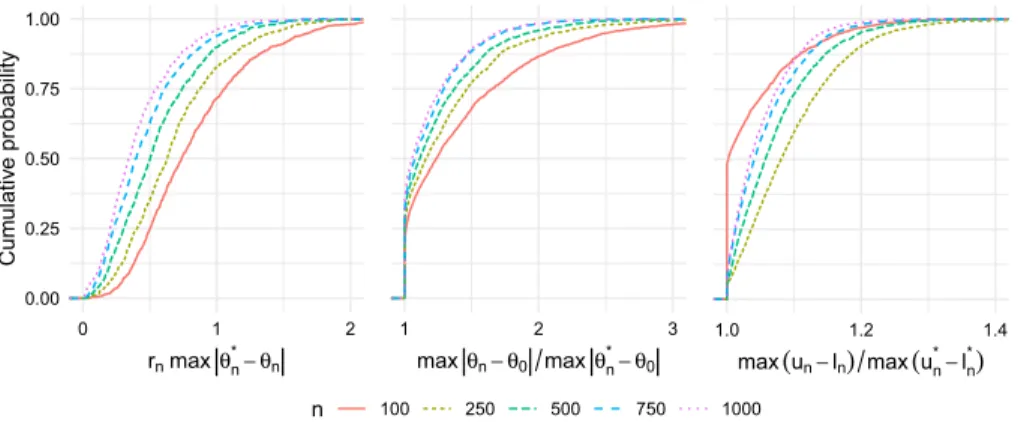
Figure 1 displays the results of this simulation study, with output from the univariate and bivariate projection approaches summarized in the top and bot-tom rows, respectively. The left column displays the empirical distribution of the scaled maximum absolute discrepancy betweenθnandθn∗for all sample sizes
studied. This plot confirms that the discrepancy between these two estimators indeed decreases faster than n−1/2, as our theory suggests. Furthermore, for
eachn, the discrepancy is larger for the two-dimensional projection.
The middle column of Figure 1 displays the empirical distribution function of the ratio between the maximum discrepancy between θn and θ0 and that of θ∗n andθ0. This plot confirms thatθ∗n is always at least as close toθ0than isθn
overTn. The maximum discrepancy between θn andθ0 can be more than 25%
larger than that betweenθn∗ andθ0in the univariate case, and up to 50% larger
in the bivariate case.
The right column of Figure 1 displays the empirical distribution function of the ratio between the maximum size of the initial uniform 95% influence
Table 1
Coverage of 95% confidence bands for the true counterfactual distribution function.
n 100 250 500 750 1000 d=1 Initial band 92.5 94.1 96.0 94.5 95.5 Monotone band 92.5 94.1 96.0 94.5 95.5 d=2 Initial band 93.9 94.0 95.0 94.6 94.9 Monotone band 95.7 95.9 95.5 95.3 95.1
function-based confidence band and that of the isotonic band. For large sam-ples, the maximal widths are often close, but for smaller samsam-ples, the initial confidence bands can be up to 50% larger than the isotonic bands, especially for the bivariate case. The empirical coverage of both bands is provided in Table1. The coverage of the isotonic band is essentially the same as the initial band for the univariate case, whereas it is slightly larger than that of the initial band in the bivariate case.
Fig 1. Summary of simulation results for G-computed distribution function. Each plot shows
cumulative distributions of a particular discrepancy over 1000 simulated datasets for different values ofn. Left panel: maximal absolute difference between the initial and isotonic estima-tors over the grid used for projecting, scaled up by root-n. Middle panel: ratio of the maximal absolute difference between the initial estimator and the truth and the maximal absolute dif-ference between the isotonic estimator and the truth. Right panel: ratio of the maximal width of the initial confidence band and the maximal width of the isotonic confidence band. The top row shows the results for the univariate projection, and the bottom row shows the results for the bivariate projection.
4.2. Example 2: Estimation of a conditional distribution function We next demonstrate the use of Theorem 2 with dimension d= 2 for drawing inference on a conditional distribution function. Suppose that the data unit is the
3048
vectorX = (A, Y), whereY is an outcome andAis now a continuous exposure. The observed data consist of independent draws (A1, Y1),(A2, Y2), . . . ,(An, Yn)
fromP0∈M, whereMis a nonparametric model. We define the parameter value θP pointwise as θP(t1, t2) := P(Y ≤t1|A=t2). Thus, θP is the conditional
distribution function of Y at t1 given A = t2. The map (t1, t2) → θP(t1, t2)
is necessarily monotone int1 for each fixedt2, and in some settings, it may be
known that it is also monotone int2for each fixedt1. This parameter completely
describes the conditional distribution ofY givenA, and can be used to obtain the conditional mean, conditional quantiles, or any other conditional parameter of interest.
For each t1, the true function θ0(t1, t2) =θP0(t1, t2) may be written as the
conditional mean ofI(Y ≤t1) givenA=t2. Hence, any method of
nonparamet-ric regression can be used to estimatet2→θ0(t1, t2) for fixed t1, and repeating
such a method over a grid of values oft1 yields an estimator of the entire
func-tion. We expect that our results would apply to many of these methods. Here, we consider the local linear estimator (Fan and Gijbels, 1996), which may be expressed as θn(t1, t2) := 1 nhn n i=1 I(Yi≤t1) s2,n(t2)−s1,n(t2) (Ai−t2) s0,n(t2)s2,n(t2)−s1,n(t2)2 K Ai−t2 hn ,
where K : R → R is a symmetric and bounded kernel function, hn → 0 is a
sequence of bandwidths, and
sj,n(t2) := 1 nhn n i=1 (Ai−t2)jK Ai−t2 hn
for j ∈ {0,1,2}. Under regularity conditions on the true distribution function
θ0, the marginal density f0 of A, the bandwidth sequence hn, and the kernel
functionK, for any fixed (t1, t2),θn satisfies
(nhn)1/2 θn(t1, t2)−θ0(t1, t2)−h2nVKb0(t1, t2) d −→N(0, SKv0(t1, t2)), whereVK:= x2K(x)dxis the variance ofK,SK := K(x)2dx, andb0(t1, t2)
andv0(t1, t2) depend on the derivatives ofθ0and onf0. Ifhn is chosen to be of
order n−1/5, the rate that minimizes the asymptotic mean integrated squared error ofθn relative toθ0, then n2/5[θn(t1, t2)−θ0(t1, t2)] converges in law to a
normal random variate with meanVKb0(t1, t2) and varianceSKv0(t1, t2). Under
stronger regularity conditions, the rate of convergence of the uniform norm
θn−θ0T can be shown to be (nhn/logn)1/2 (Hardle, Janssen and Serfling,
1988).
Theorem3cannot be used to establish (A) in this problem, sinceθnis not an
asymptotically linear estimator. Furthermore, as discussed above, recent results suggest that{rn[θn(t)−θ0(t)] :t∈T}does not converge weakly to a tight limit
condi-tion (A) can be verified directly in the context of this example under smoothness conditions on θ0 and f0 using the tail bounds for empirical processes outlined
in Section3.2. Denoting byθ0,t 2 andθ0,t2 the first and second derivatives ofθ0
with respect to its second argument, we define
Rθ(2)(t, δ) :=θ0(t1, t2+δ)−θ0(t1, t2)−δθ0,t 2(t1, t2)−
1 2δ
2θ
0,t2(t1, t2)
and R(1)f (t, δ) :=f0(t2+δ)−f0(t2)−δf0(t2), wheref0 is the derivative of f0.
We then introduce the following conditions on θ0,f0, and K:
(d) θ0,t2exists and is continuous onT, and asδ→0, supt∈T|R(2)θ (t, δ)|=o(δ2);
(e) inft∈Tf0(t)>0,f0 exists and is continuous onT, and supt∈T|R (1)
f (t, δ)|= o(δ);
(f ) K is a Lipschitz function supported on [−1,1] satisfying condition (M) of Stupfler (2016). We also define νn,t(y, a) := [I(y≤t1)−θ0(t1, a)]K a−t2 hn ; gn(t2) := s0,n(t2)s2,n(t2)−s1,n(t2)2; Rn(t) := h−n1/2 s2,n(t2) gn(t2) Gn νn,t− s1,n(t2) gn(t2) Gn (tνn,t) .
We then have the following result.
Proposition 1. If (d)–(f ) hold, nh4
n/logh−n1→ ∞andnh5n=O(1), then
sup t∈T (nhn)1/2[θn(t1, t2)−θ0(t1, t2)]− nh5n1/2 12θ0,t 2(t1, t2)K2−Rn(t) P −→0 .
Proposition 1 aids in establishing the following result, which formally es-tablishes asymptotic equivalence of the local linear estimator of a conditional distribution function and its correction obtained via isotonic regression at the ratern= (nhn)1/2.
Proposition 2. If (d)–(f ) hold andnh5
n →c∈(0,∞), then (A) holds for the
local linear estimator withrn= (nhn)1/2.
The proofs of Propositions 1 and 2 are provided in Appendix A.5. These results may also be of interest in their own right for establishing other properties of the local linear estimator.
As with the first example, we conducted a simulation study to validate our theoretical results. For samples sizesn∈ {100,250,500,750,1000}, we generated 1000 random datasets as follows. We first simulated A as a Beta(2,3) variate. GivenA=a,Y was simulated as the inverse-logistic transformation of a normal variate with mean 0.5×[1 + (a−1.2)2] and variance one.
For each simulated dataset, we estimatedθ0(y, a) for each (y, a) in an equally
esti-3050
mated the functiona→θ0(y, a) using the local linear estimator, as implemented
in the R packageKernSmooth (Wand, 2015; Wand and Jones, 1995). For each value ofy in the grid, we computed the optimal bandwidth based on the direct plug-in methodology of Ruppert, Sheather and Wand (1995) as implemented by thedpill function, and we then set our bandwidth as the average of these
y-specific bandwidths. We constructed initial confidence bands using a variable-width nonparametric bootstrap (Hall and Kang,2001).
We first note that, for all sample sizes considered, over 99% of simulations had monotonicity violations in both they- anda-directions. Figure 2 displays the results of this simulation study. The left exhibit of Figure 2 confirms that the discrepancy between θn and θ∗n decreases faster thanr−n1 =n−2/5, as our
theory suggests. The middle exhibit indicates that in roughly 50% of simulations, there is less than 5% difference between θ∗n −θ0Tn and θn −θ0Tn, but
even for n = 1000, in roughly 25% of simulations, θn∗ offers at least a 25%
improvement in estimation error. In smaller samples, the estimation error of
θ∗n is less than half that of θn in 5–10% of simulations. The rightmost exhibit
indicates that the projected confidence bands regularly reduce the uniform size of the initial bands by 10–20%. Finally, the empirical coverage of uniform 95% bootstrap-based bands and their projected versions is provided in Table2. As before, the projected band is always more conservative than the initial band, and the difference in coverage diminishes asngrows. However, the initial bands in this example are anti-conservative, even atn= 1000, likely due to the slower rate of convergence, and the corrected bands offer a much more substantial improvement in this example than in the first.
Fig 2. Summary of simulation results for conditional distribution function. The three columns
display the same results as those in Figure1.
5. Discussion
Many estimators of function-valued parameters in nonparametric and semipara-metric models are not guaranteed to respect shape constraints on the true
func-Table 2
Coverage of 95% confidence bands for the true conditional distribution function.
n 100 250 500 750 1000 Initial band 37.6 64.9 83.2 86.3 89.7 Monotone band 60.8 80.4 90.3 92.3 93.9
tion. A simple and general solution to this problem is to project the initial esti-mator onto the constrained parameter space over a grid whose mesh goes to zero fast enough with sample size. However, this introduces the possibility that the projected estimator has different properties than the original estimator. In this paper, we studied the important shape constraint of multivariate component-wise monotonicity. We provided results indicating that the projected estimator is generically no worse than the initial estimator, and that if the true function is strictly increasing and the initial estimator possesses a relatively weak type of stochastic equicontinuity, the projected estimator is uniformly asymptoti-cally equivalent to the initial estimator. We provided especially simple sufficient conditions for this latter result when the initial estimator is uniformly asymptot-ically linear, and provided guidance on establishing the key condition for kernel smoothed estimators.
We studied the application of our results in two examples: estimation of a G-computed distribution function, for use in understanding the effect of a binary exposure on an outcome when the exposure-outcome relationship is confounded by recorded covariates, and of a conditional distribution function, for use in char-acterizing the marginal dependence of an outcome on a continuous exposure. In numerical studies, we found that the projected estimator yielded improvements over the initial estimator. The improvements were especially strong in the latter example.
In our examples, we only studied corrections in dimensionsd= 1 andd= 2. In future work, it would be interesting to consider corrections in dimensions higher than 2. For example, for the conditional distribution function, it would be of interest to study multivariate local linear estimators for a continuous exposure Ataking values inRd−1 ford >2. Since tailored algorithms for com-puting the isotonic regression do not yet exist for d > 2, it would also be of interest to determine whether a version of Theorem 2 could be established for the relaxed isotonic estimator proposed by Fokianos, Leucht and Neumann (2017). Alternatively, it is possible that the uniform stochastic equicontinuity currently required by Chernozhukov, Fern´andez-Val and Galichon (2010) and Daouia and Park (2013) for asymptotic equivalence of the rearrangement- and envelope-based corrections, respectively, could be relaxed along the lines of our condition (A). Finally, our theoretical results do not give the exact asymptotic behavior of the projected estimator or projected confidence band when the true function possesses flat regions. This is also an interesting topic for future re-search.
3052
Appendix A: Technical proofs
A.1. Proof of Theorem 1
Part (i) follows from Corollary B to Theorem 1.6.1 of Robertson, Wright and Dykstra (1988). For parts (ii) and (iii), we note that by assumption
|θ∗n(t)−θ0(t)| ≤ k λk,n(t)|θn∗(sk)−θ0(sk)|+ k λk,n(t)|θ0(sk)−θ0(t)|
for everyt∈T, wherekλk,n(t) = 1, and for eachk,sk ∈Tn andsk−t ≤
2ωn. By part (i), the first term is bounded above by sups∈Tn|θn(s)−θ0(s)|. The
second term is bounded above byγ(2ωn), where we define γ(δ) := sup{|θ0(t)−θ0(s)|:t, s∈T,t−s ≤δ} .
Ifθ0is continuous onT, then it is also uniformly continuous sinceTis compact.
Therefore, γ(δ) → γ(0) = 0 as δ → 0, so that γ(2ωn)→P0 if ωn→P0. If γ(δ) =o(δα) asδ→0, thenγ(2ω
n) =oP(ωαn).
Part (iv) follows from the proof of Proposition 3 of Chernozhukov, Fern´ andez-Val and Galichon (2009), which applies to any order-preserving monotonization procedure. For the first statement of (v), by their definition as minimizers of the least-squares criterion function, we note thatt∈Tnu∗n(t) =t∈Tnun(t), and
similarly for∗n. The second statement of (v) follows from a slight modification of Theorem 1.6.1 of Robertson, Wright and Dykstra (1988). As stated, the result says thatt∈TnG(θ∗(t)−θ(t))≤t∈TnG(θ(t)−ψ(t)) for any convex function
G:R→Rand monotone functionψ, whereθ∗is the isotonic regression ofθover
Tn. A straightforward adaptation of the proof indicates that
t∈TnG(θ
∗
1(t)− θ∗2(t))≤t∈TnG(θ1(t)−θ2(t)), where nowθ∗1andθ2∗are the isotonic regressions
of θ1 and θ2 over Tn, respectively. As in Corollary B, takingG(x) = |x|p and
lettingp→ ∞yields thatθ1∗−θ2∗Tn≤ θ1−θ2Tn. Applying this withθ1=un
andθ2=n establishes the second portion of (v).
A.2. Proof of Theorem 2
We prove Theorem 2 via three lemmas, which may be of interest in their own right. The first lemma controls the size of deviations inθnover small
neighbor-hoods, and does not hinge on condition (C) holding.
Lemma 1. If (A)–(B) hold and bn=oP(r−n1), then
sup
t−s≤bn
|θn(t)−θn(s)|=oP(r−n1).
Proof of Lemma 1. In view of the triangle inequality,
|θn(t)−θn(s)| ≤ |{θn(t)−θ0(t)} − {θn(s)−θ0(s)}|+|θ0(t)−θ0(s)| .
The second lemma controls the size of neighborhoods over which violations in monotonicity can occur. Henceforth, we define
κn := sup{t−s:s, t∈T, s≤t, θn(t)≤θn(s)} .
In this lemma we again require (A) but now require (C) rather than (B).
Lemma 2. If (A) and (C) hold, then κn =oP(r−n1).
Proof of Lemma 2. Let >0 andηn :=/rn. Suppose thatκn > ηn. Then,
there exists, t∈Twiths < tandt−s> ηnsuch thatθn(s)≥θn(t). We claim
that there must also exists∗, t∗∈Twiths∗< t∗andt∗−s∗ ∈[ηn/2, ηn] such
that θn(s∗)≥θn(t∗). To see this, let J =t−s/(ηn/2) −1, and note that J ≥1. Definetj:=s+(jηn/2)(t−s)/t−sforj = 0,1, . . . , J, and settJ+1:=t.
Thus,tj< tj+1 andtj+1−tj ∈[ηn/2, ηn] for eachj= 0,1, . . . , J. Since then
J
j=0[θn(tj+1)−θn(tj)] =θn(t)−θn(s)≤0, it must be thatθn(tj+1)≤θn(tj)
for at least one j. This proves the claim.
We now have that κn > ηn implies that there exist s, t∈T with s < t and
t−s ∈[ηn/2, ηn] such thatθn(s)≥θn(t). This further implies that
{θn(t)−θ0(t)} − {θn(s)−θ0(s)} ≤ −{θ0(t)−θ0(s)} ≤ −K0t−s ≤ −K0ηn/2
by condition (B). Finally, this allows us to write
P0 κn> rn ≤P0 sup t−s≤/rn rn|[θn(t)−θ0(t)]−[θn(s)−θ0(s)]| ≥ K0 2 .
By condition (A), this probability tends to zero for every >0, which completes the proof.
Our final lemma bounds the maximal absolute deviation betweenθn∗ andθn
over the grid Tn in terms of the supremal deviations ofθn over neighborhoods
smaller thanκn. This lemma does not depend on any of the conditions (A)–(C).
Lemma 3. It holds that maxt∈Tn|θn∗(t)−θn(t)| ≤sups−t≤κn|θn(s)−θn(t)|.
Proof of Lemma 3. By Theorem 1.4.4 of Robertson, Wright and Dykstra (1988), for anyt∈Tn, θ∗n(t) = max U∈Ut min L∈Lt θn(U∩L) = min L∈Lt max U∈Ut θn(U∩L),
where, for any finite setS⊆Tn,θn(S) is defined as|S|−1
s∈Sθn(s). The sets U range over the collection Ut of upper sets ofTn containingt, whereU ⊆Tn
is called an upper set if t1 ∈U, t2∈Tn andt1≤t2 impliest2∈U. The setsL
range over the collection Lt of lower sets ofTn containingt, where L⊆Tn is
called a lower set ift1∈L, t2∈Tn andt2≤t1 impliest2∈L.
Let Ut := {s : s ≥ t} and Lt := {s : s ≤ t}. First, suppose there exists L0 ∈ Lt and s0 ∈ L0 with s0 > t and t−s0 > κn. Then, we claim that