Batched Stochastic Gradient Descent with Weighted Sampling

Scholarship @ Claremont

CMC Faculty Publications and Research

CMC Faculty Scholarship

8-30-2016

Batched Stochastic Gradient Descent with

Weighted Sampling

Deanna Needell

Rachel Ward

University of Texas at Austin

This Article - preprint is brought to you for free and open access by the CMC Faculty Scholarship at Scholarship @ Claremont. It has been accepted for inclusion in CMC Faculty Publications and Research by an authorized administrator of Scholarship @ Claremont. For more information, please [email protected].

Recommended Citation

DEANNA NEEDELL AND RACHEL WARD

ABSTRACT. We analyze a batched variant of Stochastic Gradient Descent (SGD) with weighted sampling dis-tribution for smooth and non-smooth objective functions. We show that by distributing the batches com-putationally, a significant speedup in the convergence rate is provably possible compared to either batched sampling or weighted sampling alone. We propose several computationally efficient schemes to approxi-mate the optimal weights, and compute proposed sampling distributions explicitly for the least squares and hinge loss problems. We show both analytically and experimentally that substantial gains can be obtained.

1. MATHEMATICALFORMULATION We consider minimizing an objective function of the form

F(x)=1 n n X i=1 fi(x)=Efi(x). (1.1)

One important such objective function is the least squares objective for linear systems. Given ann×m

matrixAwith rowsa1, . . . ,anand a vectorb∈Rn, one searches for the least squares solutionxLSgiven by

xLS def =argmin x∈Rm 1 2kAx−bk 2 2=argmin x∈Rm 1 n n X i=1 n 2(bi− 〈ai,x〉) 2 =argmin x∈Rm E fi(x), (1.2)

where the functionals are defined byfi(x)=n₂(bi− 〈ai,x〉)2.

Another important example is the setting of support vector machines where one wishes to minimize the hinge loss objective given by

xH L def =argmin w∈Rm 1 n n X i=1 [1−yi〈w,xi〉]++λ 2kwk 2 2. (1.3)

Here, the data is given by the matrix X with rows x1, . . . ,xn and the labels yi ∈{−1, 1}. The function

[z]+

def

=max(0,z) denotes the positive part. We view the problem (1.3) in the form (1.1) with fi(w)=

[1−yi〈w,xi〉]+and regularizerλ2kwk22.

The stochastic gradient descent (SGD) method solves problems of the form (1.1) by iteratively moving in the gradient direction of a randomly selected functional. SGD can be described succinctly by the update rule:

xk+1←xk−γ∇fik(xk),

where indexikis selected randomly in thekth iteration, and an initial estimationx0is chosen arbitrarily.

Typical implementations of SGD select the functionals uniformly at random, although if the problem at hand allows a one-pass preprocessing of the functionals, certainweightedsampling distributions pre-ferring functionals with larger variation can provide better convergence (see e.g. [NSW16, ZZ15] and references therein). In particular, Needell et al. show that selecting a functional with probability pro-portional to the Lipschitz constant of its gradient yields a convergence rate depending on theaverageof all such Lipschitz constants, rather than the supremum [NSW16]. An analogous result in the same work shows that for non-smooth functionals, the probabilities should be chosen proportional to the Lipschitz constant of the functional itself.

Date: August 30, 2016.

1

Another variant of SGD utilizes so-calledmini-batches; in this variant, a batch of functionals is se-lected in each iteration rather than a single one [CSSS11, AD11, DGBSX12, TBRS13]. The computations over the batches can then be run in parallel and speedups in the convergence are often quite significant.

Contribution.Our main contribution is to propose a weighted sampling scheme to be used in mini-batch SGD. We show that when the mini-batches can be implemented in parallel, significant speedup in con-vergence is possible. In particular, we analyze the concon-vergence using computed distributions for the least squares and hinge loss objectives, the latter being especially challenging since it is non-smooth. We demonstrate theoretically and empirically that weighting the distribution and utilizing batches of functionals per iteration together form a complementary approach to accelerating convergence.

Organization.We next briefly discuss some related work on SGD, weighted distributions, and batch-ing methods. We then combine these ideas into one cohesive framework and discuss the benefits in various settings. Section 2 focuses on the impact of weighting the distribution. In Section 3 we analyze SGD with weighting and batches for smooth objective functions, considering the least squares objective as a motivating example. We analyze the non-smooth case along with the hinge loss objective function in Section 4. We display experimental results for the least squares problem in Section 5 that serve to highlight the relative tradeoffs of using both batches and weighting, along with different computational approaches. We conclude in Section 6.

Related work.Stochastic gradient descent, stemming from the work [RM51], has recently received re-newed attention for its effectiveness in treating large-scale problems arising in machine learning [BB11, Bot10, NJLS09, SSS08]. Importance sampling in stochastic gradient descent, as in the case of mini-batching (which we also refer to simply asbatchinghere), also leads to variance reduction in stochastic gradient methods and, in terms of theory, leads to improvement of the leading constant in the complex-ity estimate, typically via replacing the maximum of certain data-dependent quantities by their average. Such theoretical guarantees were shown for the case of solving least squares problems where stochastic gradient descent coincides with the randomized Kaczmarz method in [SV09]. This method was extended to handle noisy linear systems in [Nee10]. Later, this strategy was extended to the more general setting of smooth and strongly convex objectives in [NSW16], building on an analysis of stochastic gradient de-scent in [BM11]. Later, [ZZ15] considered a similar importance sampling strategy for convex but not necessarily smooth objective functions. Importance sampling has also been considered in the related setting of stochastic coordinate descent/ascent methods [Nes12, RT15, QRZ15, CQR15]. Other papers exploring advantages of importance sampling in various adaptations of stochastic gradient descent in-clude but are not limited to [LS13, SRB13, XZ14, DB15].

Mini-batching in stochastic gradient methods refers to pooling together several random examples in the estimate of the gradient, as opposed to just a single random example at a time, effectively re-ducing the variance of each iteration [SSSSC11]. On the other hand, each iteration also increases in complexity as the size of the batch grows. However, if parallel processing is available, the computation can be done concurrently at each step, so that the “per-iteration cost" with batching is not higher than without batching. Ideally, one would like the consequence of using batch sizeb to result in a conver-gence rate speed-up by factor ofb, but this is not always the case [BCNW12]. Still, [TBRS13] showed that by incorporating parallelization or multiple cores, this strategy can only improve on the conver-gence rate over standard stochastic gradient, and can improve the converconver-gence rate by a factor of the batch size in certain situations, such as when the matrix has nearly orthonormal rows. Other recent pa-pers exploring the advantages of mini-batching in different settings of stochastic optimization include [CSSS11, DGBSX12, NW13, KLRT16, LZCS14].

The recent paper [CR16] also considered the combination of importance sampling and mini-batching for a stochastic dual coordinate ascent algorithm in the general setting of empirical risk minimization, wherein the function to minimize is smooth and convex. There the authors provide a theoretical optimal sampling strategy that is not practical to implement but can be approximated via alternating minimiza-tion. They also provide a computationally efficient formula that yields better sample complexity than

uniform mini-batching, but without quantitative bounds on the gain. In particular, they do not pro-vide general assumptions under which one achieves provable speed-up in convergence depending on an average Lipschitz constant rather than a maximum.

For an overview of applications of stochastic gradient descent and its weighted/batched variants in large-scale matrix inversion problems, we refer the reader to [GR16].

2. SGDWITH WEIGHTING

Recall the objective function (1.1). We assume in this section that the functionFand the functionals

fisatisfy the following convexity and smoothness conditions:

Convexity and smoothness conditions

(1) Each fi is continuously differentiable and the gradient function∇fi has Lipschitz constant bounded byLi:k∇fi(x)− ∇fi(y)k2≤Likx−yk2for all vectorsxandy.

(2) Fhas strong convexity parameterµ; that is,〈x−y,∇F(x)− ∇F(y)〉 ≥µkx−yk22for all vectors

xandy.

(3) At the unique minimizerx_∗=argminF(x), the average gradient norm squaredk∇fi(x_∗)k22is

not too large, in the sense that 1 n n X i=1 k∇fi(x_∗)k22≤σ2.

An unbiased gradient estimate forF(x) can be obtained by drawingiuniformly from [n]def={1, 2, . . . ,n} and using∇fi(x) as the estimate for∇F(x). The standard SGD update with fixed step sizeγis given by

xk+1←xk−γ∇fik(xk) (2.1)

where eachikis drawn uniformly from [n]. The idea behind weighted sampling is that, by drawingifrom

a weighted distributionD(p)={p(1),p(2), . . . ,p(n)} over [n], the weighted sample _p(1_i

k)∇fik(xk) is still an

unbiased estimate of the gradient∇F(x). This motivates the weighted SGD update xk+1←xk− γ

np(ik)∇fik(xk), (2.2)

In [NSW16], a family of distributionsD(p)whereby functionsfiwith larger Lipschitz constants are more

likely to be sampled was shown to lead to an improved convergence rate in SGD over uniform sampling. In terms of the distancekxk−x∗k22of thekth iterate to the unique minimum, starting from initial distance

ε0= kx0−x∗k22, Corollary 3.1 in [NSW16] is as follows.

Proposition 2.1. Assume the convexity and smoothness conditions are in force. For any desiredε>0, and using a stepsize of

γ= µε

4(εµ_n1Pn

i=1Li+σ2)

,

we have that after

k=4 log(2ε0/ε) Ã₁ n Pn i=1Li µ + σ2 µ2_ε ! (2.3)

iterations of weighted SGD(2.2)with weights

p(i)= 1 2n+ 1 2n· Li 1 n P iLi , (2.4)

Remark. This should be compared to the result for uniform sampling SGD [NSW16]: using step-sizeγ=

µε

4(εµ(supiLi)+σ2), one obtains the comparable error guaranteeEkxk−x∗k

2

2≤εafter a number of iterations

k=2 log(2ε0/ε) µ_sup iLi µ + σ2 µ2_ε ¶ . (2.5)

Since the average Lipschitz constant_n1P

iLiis always at most supiLi, and can be up tontimes smaller

than sup_iLi, SGD with weighted sampling requires twice the number of iterations of uniform SGD in the worst case, but can potentially converge much faster, specifically, in the regime where

σ2 µ2_ε≤ 1 n Pn i=1Li µ ¿ sup_iLi µ .

3. MINI-BATCHSGDWITH WEIGHTING:THE SMOOTH CASE

Here we present a weighting and mini-batch scheme for SGD based on Proposition 2.1. For practical purposes, we assume that the functions fi(x) such thatF(x)=_n1Pn_i=1fi(x) are initially partitioned into

fixed batches of sizeband denote the partition by {τ1,τ2, . . .τd} where|τi| =bfor alli<dandd= dn/be

(for simplicity we will henceforth assume thatd=n/bis an integer). We will randomly select from this pre-determined partition of batches; however, our analysis extends easily to the case where a batch of sizeb is randomly selected each time from the entire set of functionals. With this notation, we may re-formulate the objective given in (1.1) as follows:

F(x)= 1 d d X i=1 g_τi(x)=Egτi(x),

where now we writeg_τi(x)=

1

b P

j∈τifj(x). We can apply Proposition 2.1 to the functionalsgτi, and select

batchτiwith probability proportional the Lipschitz constant of∇gτi (or ofgτi in the non-smooth case,

see Section 4). Note that

• The strong convexity parameterµfor the functionFremains invariant to the batching rule.

• The residual errorσ2_τsuch that_d1Pd

i=1k∇gτi(x∗)k

2

2≤σ2τcan onlydecreasewith increasing batch

size, since σ2 τ= 1 d d X k=1 k1 b∇ Ã X k∈τi fk(x) ! k22≤ 1 n n X i=1 k∇fi(x)k22≤σ 2_.

• The average Lipschitz constantL_τ=_d1Pd

i=1Lτi of the gradients of the batched functionsgτi can

onlydecreasewith increasing batch size, since by the triangle inequality,Lτi ≤

1 b P k∈τiLk, and thus 1 d d X i=1 L_τi≤ 1 n n X k=1 Lk=L.

Incorporating these observations, applying Proposition 2.1 in the batched weighted setting implies that incorporating weighted sampling and mini-batching in SGD results in a convergence rate that equals or improves on the rate obtained using weights alone:

Theorem 3.1. Assume that the convexity and smoothness conditions on F(x)=_n1Pn

i=1fi(x)are in force.

Consider the d=n/b batches g_τi(x)=

1

b P

k∈τi fk(x), and the batched weighted SGD iteration

xk+1←xk− γ d·p(τik)

∇g_τik(xk) where batchτiis selected at iteration k with probability

p(τi)= 1 2d+ 1 2d· L_τi L_τ. (3.1)

For any desiredε, and using a stepsize of

γ= µε

4(εµL_τ+σ2τ)

,

we have that after a number of iterations

k=4 log(2ε0/ε) Ã L_τ µ + σ2 τ µ2_ε ! ,

the following holds in expectation with respect to the weighted distribution(3.1):E(p)kxk−x∗k22≤ε.

Remark. Since à L_τ µ + σ2 τ µ2_ε ! ≤ à L µ+ σ2 µ2_ε ! ,

this implies that batching and weighting can only improve the convergence rate of SGD compared to weighting alone.

To completely justify the strategy of batching + weighting, we must also take into account the precom-putation cost in computing the weighted distribution (3.1), which increases with the batch sizeb. In the next section, we refine Theorem 3.1 precisely this way in the case of the least squares objective, where we can quantify more precisely the gain achieved by weighting and batching. We give several explicit bounds and sampling strategies on the Lipschitz constants in this case that can be used for computa-tionally efficient sampling.

3.1. Least Squares Objective. Consider the least squares objective

F(x)=1 2kAx−bk 2 2= 1 n n X i=1 fi(x),

wherefi(x)=n2(bi− 〈ai,x〉)2. We assume the matrixAhas full row-rank, so that there is a unique

mini-mizerx_∗to the least squares problem:

xLS=x∗=arg min_x kAx−bk22.

Note that the convexity and smoothness conditions are satisfied for such functions. Indeed, observe that

∇fi(x)=n(〈ai,x〉 −bi)ai, and

(1) The individual Lipschitz constants are bounded byLi=nkaik2₂, and the average Lipschitz

con-stant by_n1P

iLi= kAk2F(wherek · kFdenotes the Frobenius norm),

(2) The strong convexity parameter isµ= _kA−11_k2 (where kA−1k =σ−_min1 (A) is the reciprocal of the

smallest singular value ofA), (3) The residual isσ2=nP

ikaik22|〈ai,x∗〉 −ai|2.

In the batched setting, we compute

g_τi(x)=1 b X k∈τi fk(x)= n 2b X k∈τi (bk− 〈ak,x〉)2= d 2kAτix−bτik 2 2, (3.2)

where we have writtenA_τito denote the submatrix ofAconsisting of the rows indexed byτi.

Denote byσ2_τthe residual in the batched setting. Since∇g_τi=dP

k∈τi(〈ak,x〉 −bk)ak, σ2 τ=_d1 d X i=1 k∇g_τi(x∗)k 2 2=d d X i=1 kX k∈τi (〈ak,x∗〉 −bk)akk22 =d d X i=1 kA∗_τi(A_τix_∗−b_τi)k22≤d d X i=1 kA_τik2kA_τix_∗−b_τik22.

Denote byL_τithe Lipschitz constant of∇gτi. Then we also have L_τi=sup x,y k∇g_τi(x)− ∇g_τi(y)k2 kx−yk2 =n bsupx,y kP k∈τi £ (〈ak,x〉 −bk)ak−(〈ak,y〉 −bk)ak ¤ k2 kx−yk2 =n bsupz kP k∈τi〈ak,z〉akk2 kzk2 =n bsupz kA∗_τiA_τizk2 kzk2 =n bkA ∗ τiAτik =dkA_τik22,

where we have writtenkBkto denote the spectral norm of the matrixB, andB∗the adjoint of the matrix. We see thus that if there exists a partition such that kA_τikare as small as possible for allτi in the partition, then bothσ2_τ and L_τ= _d1P

iLτi are decreased by a factor of the batch size b compared to the

unbatched setting.These observations are summed up in the following corollary of Theorem 3.1 for the least squares case.

Corollary 3.2. Consider F(x)= 1₂kAx−bk22= 12

Pd

i=1kAτix−bτik

2

2. Consider the batched weighted SGD

iteration xk+1←xk− γ p(τi) X j∈τi (〈aj,xk〉 −bj)aj. (3.3) with weights p(τi)= b 2n+ 1 2· kA_τik 2 Pd i=1kAτik 2. (3.4)

For any desiredε, and using a stepsize of

γ= 1 4ε εPd i=1kAτik 2_+dkA−1_k2Pd i=1kAτik 2_kA τix∗−bτik 2 2 , (3.5)

we have that after

k=4 log(2ε0/ε) Ã kA−1k2 d X i=1 kAτik 2 +dkA −1 k4Pd i=1kAτik 2 kAτix∗−bτik 2 2 ε ! (3.6) iterations of (3.3),E(p)kxk−x∗k22≤εwhereE (p)_[

·]means the expectation with respect to the index at each iteration drawn according to the weighted distribution(3.4).

This corollary suggests a heuristic for batching and weighting in SGD for least squares problems, in order to optimize the convergence rate:

(1) Find a partitionτ1,τ2, . . . ,τdthat roughly minimizesPd_i=1kAτik

2

2among all such partitions

(2) Apply the weighted SGD algorithm (2.2) using weights

p(τi)= 1 2d+ 1 2· kAτik 2 2 Pd i=1kAτik 2 2 .

We can compare the results of Corollary 3.2 to the results for weighted SGD when a single functional is selected in each iteration, where the number of iterations to achieve expected errorεis

k=4 log(2ε0/ε) Ã kA−1k2 n X i=1 kaik2+ nkA−1 k4Pn i=1kaik 2 k〈ai,x∗〉 −bik22 ε ! ; (3.7)

That is, the ratio between the standard weighted number of iterationskst and in (3.7) and the batched weighted number of iterationskbat chin (3.6) is

kst and kbat ch = εPn i=1kaik2+nkA−1k2 Pn i=1kaik2k〈ai,x∗〉 −bik22 εPd i=1kAτik2+dkA−1k2 Pd i=1kAτik2kAτix∗−bτik 2 2 (3.8)

In case the least squares residual error is uniformly distributed over thenindices, that is,k〈ai,x∗〉−bik22≈ 1

nkAx∗−bk

2_{for eachi}

∈[n], this factor reduces to

kst and kbat ch = kAk 2 F Pd i=1kAτik2 (3.9) It follows thus that the combination of batching and weighting in this setting always reduces the iteration complexity compared to weighting alone, and can result in up to a factor ofbspeed-up:

1≤kst and

kbat ch ≤ b;

In the remainder of this section, we consider several families of matrices where the maximal speedup is achieved, kst and

kbat ch ≈b. We also take into account the computational cost of computing the normskAτik

2 2

which determine the weighted sampling strategy.

Orthonormal systems: It is clear that the advantage of mini-batching is strongest when the rows of Ain each batch are orthonormal. In the extreme case whereAhas orthonormal rows, we have

L_τ= d X i=1 kA∗_τiA_τik =n b = 1 bL.

Thus for orthonormal systems, we gain a factor ofbby using mini-batches of sizeb. However, there is little advantage to weighting in this case as all Lipschitz constants are the same.

Incoherent systems: More generally, the advantage of mini-batching is strong when the rows ai

within any particular batch arenearly orthogonal. Suppose that each of the batches is well-conditioned in the sense that

n X i=1 kaik22≥C0n, kAτ∗iAτik = kAτiA ∗ τik ≤C, i=1, . . . ,d, (3.10)

For example, ifA∗_{has therestricted isometry property[CT05] of levelδat sparsity levelb, (3.10)}

holds withC≤1+δ. Alternatively, ifAhas unit-norm rows and is incoherent, i.e. maxi6=j|〈ai,aj〉| ≤

α

b−1, then (3.10) holds with constantC≤1+αby Gershgorin circle theorem.

If the incoherence condition (3.10) holds, we gain a factor ofbby using weighted mini-batches of sizeb: Lτ= d X i=1 kA∗_τiAτik ≤C n b ≤ C C0 L b.

Incoherent systems, variable row norms: More generally, consider the case where the rows of A are nearly orthogonal to each other, but not normalized as in (3.10). We can then writeA=DΨ, whereDis ann×ndiagonal matrix with entrydi i= kaik2, andΨwith normalized rows satisfies

kΨ∗_τiΨτik = kΨτiΨ ∗

τik ≤C, i=1, . . . ,d,

In this case, we have kA∗_τ iAτik = kAτiA ∗ τik = kDτiΨτiΨ ∗ τiDτik ≤max k∈τi kakk22kΨτiΨ ∗ τik ≤Cmax k∈τi kakk22, i=1, . . . ,d. (3.11) Thus, L_τ= d X i=1 kA∗_τiA_τik ≤C d X i=1 max k∈τi kakk22. (3.12)

In order to minimize the expression on the right hand side over all partitions into blocks of size

b, we partition the rows ofAaccording to the order of the decreasing rearrangement of their row norms. This batching strategy results in a factor ofbgain in iteration complexity compared to weighting without batching:

L_τ≤C d X i=1 ka((i−1)b+1)k22 ≤ C b−1 n X i=1 kaik22 ≤C 0 b L. (3.13)

We now turn to the practicality of computing the distribution given by the constantsL_τi. We propose

several options to efficiently compute these values given the ability to parallelize overbcores.

Max-norm: The discussion above suggests the use of the maximum row norm of a batch as a proxy for the Lipschitz constant. Indeed, (3.11) shows that the row norms give an upper bound on these constants. Then, (3.13) shows that up to a constant factor, such a proxy still has the potential to lead to an increase in the convergence rate by a factor ofb. Of course, computing the maximum row norm of each batch costs on the order ofmnflops (the same as the non-batched weighted SGD case).

Power method: In some cases, we may utilize the power method to approximatekA∗_τiA_τik

effi-ciently. Suppose that for each batch we can approximate this quantity by ˆQ_τi. Classical results on the power method allow one to approximate the norm to within an arbitrary additive error, with a number of iterations that depends on the spectral gap of the matrix. An alternative approach, that we consider here, can be used to obtain approximations leading to amultiplicativefactor difference in the convergence rate, without dependence on the eigenvalue gapsλ1/λ2 within

batches. For example, [KL96, Lemma 5] show that with high probability with respect to a ran-domized initial direction to the power method, afterT ≥ε−1log(ε−1b) iterations of the power method, one can guarantee that

kA∗_τiA_τik ≥Qˆτi≥

kA∗

τiAτik

1+ε .

Atb2computations per iteration of the power method, the total computational cost (to compute all quantities in the partition), shared over allb cores, isbε−1log(ε−1log(b)). This is actually potentially muchlowerthan the cost to compute all row norms Li = kaik22 as in the standard

non-batched weighted method. In this case, the power method yields

L_τ≥b n d X i=1 n bQˆτi≥ L_τ 1+ε, for a constantε.

4. MINI-BATCHSGDWITH WEIGHTING:THE NON-SMOOTH CASE

We next present analogous results to the previous section for objectives which are strongly convex but lack the smoothness assumption. Like the least squares objective in the previous section, our motivating example here will be the support vector machine (SVM) with hinge loss objective.

A classical result (see e.g. [Nes04, SZ12, RSS12]) for SGD establishes a convergence bound of SGD with non-smooth objectives. In this case, rather than taking a step in the gradient direction of a functional, we move in a direction of a subgradient. Instead of utilizing the Lipschitz constants of the gradient terms, we utilize the Lipschitz constants of the actual functionals themselves. Concretely, a classical bound is of the following form.

Proposition 4.1. Let the objective F(x)=Egi(x)with minimizerx_?be aµ-strongly convex (possibly non-smooth) objective. Run SGD using a subgradient hiof a randomly selected functional giat each iteration. Assume thatEhi∈∂F(xk)and that

max

x,y

kgi(x)−gi(y)k

kx−yk ≤maxx khi(x)k ≤Gi.

Set G2_=E(G2

i). Using step sizeγ=γk=1/(µk), we have E[F(xk)−F(x?)]≤CG

2_(1+logk)

µk , (4.1)

where C is an absolute constant.

Such a result can be improved by utilizing averaging of the iterations; for example, ifx_kαdenotes the average of the lastαkiterates, then the convergence rate bound (4.1) can be improved to:

E[F(xk)−F(x?)]≤ CG2³_1+log 1 min(α,(1+1/k)−α) ´ µk ≤ CG2³_1+log 1 min(α,1−α) ´ µk .

Settingm_α=min(α, 1−α), we see that to obtain an accuracy ofE[F(xk)−F(x?)]≤ε, we need k≥CG

2_m

α

µε .

In either case, it is important to notice the dependence onG2_=E(G2

i). By using weighted sampling

with weightsp(i)=Gi/P

iGi, we can improve this dependence to one on (G)2, whereG=EGi [NSW16,

ZZ15]. SinceG2_−(G)2_{=Var(Gi), this improvement reduces the dependence by an amount equal to the}

variance of the Lipschitz constantsGi. Like in the smooth case, we now consider not only weighting the distribution, but also by batching the functionalsgi. This yields the following result, which we analyze for the specific instance of SVM with hinge loss below.

Theorem 4.2. Instate the assumptions and notation of Proposition 4.1. Consider the d =n/b batches g_τi(x)=

1

b P

j∈τigj(x), and assume each batch gτi has Lipschitz constant Gτi. Write Gτ=EGτi. Run the

weighted batched SGD method with averaging as described above, with step sizeγ/p(τi). For any desired

ε, it holds that after

k=C(Gτ)

2_m

α

µε

iterations with weights

p(τi)= G_τi

P jGτj

, (4.2)

we haveE(p)[F(xk)−F(x?)]≤εwhereE(p)[·]means the expectation with respect to the index at each iter-ation drawn according to the weighted distribution(4.2).

Proof. Applying weighted SGD with weights p(τi), we re-write the objectiveP(x)=E¡gi(x)¢asP(x)= E(p)¡ ˆ g_τi(x) ¢ , where ˆ g_τi(x)= Ã 1 n X j G_τj ! Ã 1 G_τi X j∈τi gj(x) ! = Ã b n X j G_τj !_µ gτi(x) G_τi ¶ . Then, the Lipschitz constant ˆGiof ˆgτiis bounded above by ˆGi=

b n P jGτj, and so E(p)_Gˆ2 i = X i G_τi P jGτj à b n X j G_τj !2 = à b n X j G_τj !2 =(EG_τi) 2 =(G_τ)2. We now formalize these bounds and weights for the SVM with hinge loss objective. Other objec-tives such as L1 regression could also be adapted in a similar fashion, e.g. utilizing an approach as in [YCRM16].

4.1. SVM with Hinge Loss. We now consider the SVM with hinge loss problem as a motivating example for using batched weighted SGD for non-smooth objectives. Recall the SVM with hinge loss objective is

P(x) :=1 n n X i=1 [yi〈x,ai〉]++λ 2kxk 2 2=Egi(x), (4.3)

whereyi∈{±1}, [u]₊=max(0,u), and

gi(x)=[yi〈x,ai〉]++λ

2kxk

2 2.

This is a key example where the components are (λ-strongly) convex but no longer smooth. Still, eachgi

has a well-defined subgradient:

∇gi(x)=χi(x)yiai+λx,

whereχi(x)=1 ifyi〈x,ai〉 <1 and 0 otherwise. It follows thatgiis Lipschitz and its Lipschitz constant is

bounded by

Gi:=max

x,y

kgi(x)−gi(y)k

kx−yk ≤maxx k∇gi(x)k ≤ kaik2+λ.

As shown in [ZZ15], [NSW16], in the setting of non-smooth objectives of the form (4.3), where the com-ponents are not necessarily smooth, but eachgiisGi-Lipschitz, the performance of SGD depends on the

quantityG2_=E[G2

i]. In particular, the iteration complexity depends linearly onG2.

For the hinge loss example, we have calculated that

G2₌ 1 n n X i=1 (kaik2+λ)2≤2λ2+ 2 n n X i=1 kaik22.

Incorporating (non-batch) weighting to this setting, as discussed in [NSW16], reduces the iteration com-plexity to depend linearly on (G)2=(E[Gi])2, which is at mostG2_{and can be as small as} 1

nG2. For the

hinge loss example, we have

(G)2= Ã λ+1 n n X i=1 kaik2 !2 .

We note here that one can incorporate the dependence on the regularizer termλ₂kxk2₂in a more optimal way by bounding the functional norm only over the iterates themselves, as in [TBRS13, RSS12]; however, we choose a crude upper bound on the Lipschitz constant here in order to maintain a dependence on theaverageconstant rather than themaximum, and only sacrifice a constant factor.

4.1.1. Batched sampling. The paper [TBRS13] considered batched SGD for the hinge loss objective. For batchesτiof sizeb, letgτi=λ2kxk22+

1 b P k∈τi[yk〈x,ak〉]+and observe P(x) :=1 n n X i=1 [yi〈x,ai〉]++λ 2kxk 2 2=Egτi(x).

We now bound the Lipschitz constantG_τfor a batch. Letχ=χk(x) andAτhave rowsykak fork∈τ. We

have max x ° ° ° ° ° 1 b X k∈τi χk(x)ykak ° ° ° ° ° 2 =max x v u u t * 1 b X k∈τi χk(x)ykak, 1 b X k∈τi χk(x)ykak + =1 bmaxx q χT_AτA∗ τχ ≤1 bmaxx q χT_A τA∗τχ ≤1 b q bkA_τA∗ τk =p1 bkAτk, (4.4) and thereforeG_τ≤p1

bkAτk+λ. Thus, for batched SGD without weights, the iteration complexity depends

linearly on G2_τ=b n d X i=1 G_τ2_i ≤2λ2+2 n d X i=1 kA_τik 2 =2λ2+2 n d X i=1 kA∗_τiA_τik.

Even without weighting, we already see potential for drastic improvements, as noted in [TBRS13]. For example, in the orthonormal case, wherekA∗_τiA_τik =1 for eachτi, we see that with appropriately chosen

λ,G_τ2is on the order of 1_b, which is a factor ofbtimes smaller thanG2_{≈1. Similar factors are gained for}

the incoherent case as well, as in the smooth setting discussed above. Of course, we expect even more gains by utilizing both batching and weighting.

4.1.2. Weighted batched sampling. Incorporating weighted batched sampling, where we sample batch τi with probability proportional toGτ, the iteration complexity is reduced to a linear dependence on

(G_τ)2, as in Theorem 4.2. For hinge loss, we calculate (G_τ)2= Ã b n d X i=1 G_τi !2 ≤ Ã b n d X i=1 1 p bkAτik +λ !2 = Ã λ+ p b n d X i=1 kA_τik !2 . We thus have the following guarantee for the hinge loss objective.

Corollary 4.3. Consider P(x)=1_nPn

i=1[yi〈x,ai〉]++λ2kxk 2

2. Consider the batched weighted SGD iteration

xk+1←xk− 1 µkp(τi) Ã λxk+ 1 b X j∈τi χj(xk)yjaj ! , (4.5)

whereχj(x)=1if yj〈x,aj〉 <1and0otherwise. LetAτhave rows yjajfor j∈τ. For any desiredε, we have that after k= Cmin(α, 1−α)³λ+ p b n Pd i=1kAτik ´2 λε (4.6)

iterations of (4.5)with weights

p(τi)= k A_τik +λ p b n p bλ+ P jkAτjk , (4.7) it holds thatE(p)[P(xk)−P(x_∗)]≤ε. 5. EXPERIMENTS

In this section we present some simple experimental examples that illustrate the potential of utilizing weighted mini-batching. We consider several test cases as illustration.

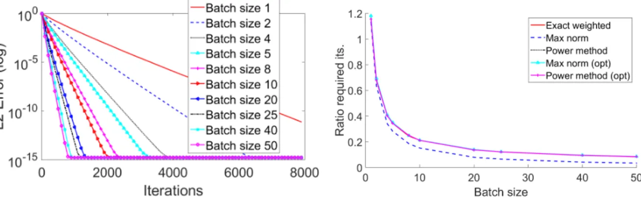
Gaussian linear systems: The first case solves a linear systemAx=b, whereAis a matrix with i.i.d. standard normal entries (as isx, andb is their product). In this case, we expect the Lipschitz constants of each block to be comparable, so the effect of weighting should be modest. However, the effect of mini-batching in parallel of course still appears. Indeed, Figure 1 (left) displays the convergence rates in terms of iterations for various batch sizes, where each batch is selected with probability as in (3.4). When batch updates can be run in parallel, we expect the convergence behavior to mimic this plot (which displays iterations). We see that in this case, larger batches yield faster convergence. In these simulations, the step sizeγwas set as in (3.5) (approximations for Lipschitz constants also apply to the step size computation) for the weighted cases and set to the optimal step size as in [NSW16, Corollary 3.2] for the uniform cases. Behavior using uni-form selection is very similar (not shown), as expected in this case since the Lipschitz constants are roughly constant. Figure 1 (right) highlights the improvements in our proposed weighted batched SGD method versus the classical, single functional and unweighted, SGD method. The power method refers to the method discussed at the end of Section 3, and max-norm method refers to the approximation using the maximum row norm in a batch, as in (3.11). The notation “(opt)” signifies that the optimal step size was used, rather than the approximation; otherwise in all cases both the sampling probabilities (3.4) and step sizes (3.5) were approximated using the approximation scheme given. Not suprisingly, using large batch sizes yields significant speedup.

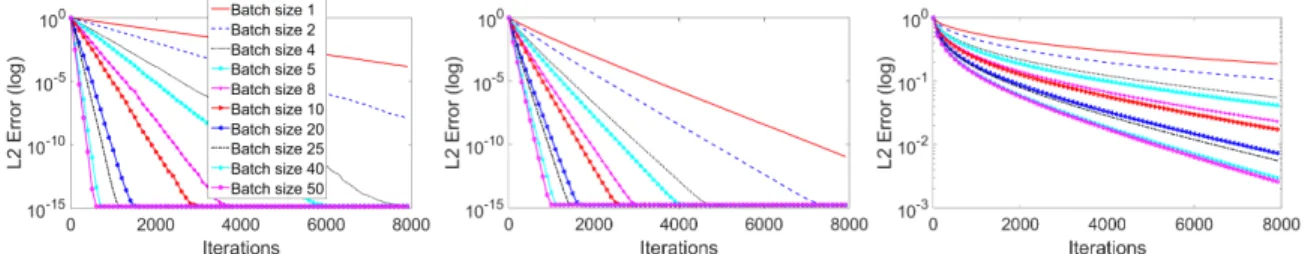
Gaussian linear systems with variation: We next test systems that have more variation in the dis-tribution of Lipschitz constants. We construct a matrix Aof the same size as above, but whose entries in thekth row are i.i.d. normally distributed with mean zero and variancek2. We now ex-pect a large effect both from batching and from weighting. In our first experiment, we select the fixed batches randomly at the onset, and compute the probabilities according to the Lipschitz constants of those randomly selected batches, as in (3.4). The results are displayed in the left plot of Figure 2. In the second experiment, we batch sequentially, so that rows with similar Lipschitz constants (row norms) appear in the same batch, and again utilized the weighted sampling. The results are displayed in the center plot of Figure 2. Finally, the right plot of Figure 2 shows con-vergence when batching sequentially and then employing uniform (unweighted) sampling. As our theoretical results predict, batching sequentially yields better convergence, as does utilizing weighted sampling.

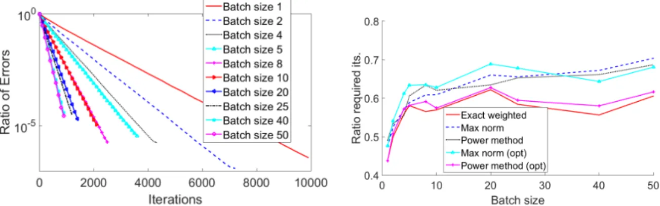
Since this type of system nicely highlights the effects of both weighting and batching, we per-formed additional experiments using this type of system. Figure 3 highlights the improvements gained by using weighting. In the left plot, we see that for all batch sizes improvements are ob-tained by using weighting, even more so than in the standard normal case, as expected (note that we cut the curves off when the weighted approach reaches machine precision). In the right plot, we see that the number of iterations to reach a desired threshold is also less using the various

weighting schemes; we compare the sampling method using exact computations of the Lipshitz constants (spectral norms), using the maximum row norm as an approximation as in (3.11), and using the power method (using number of iterations equal to²−1log(²−1b) with²=0.01). Step sizeγused on each batch was again set as in (3.5) (approximations for Lipschitz constants also apply to the step size computation) for the weighted cases and as in [NSW16, Corollary 3.2] for the uniform cases. For cases when the exact step size computation was used rather than the corresponding approximation, we write “(opt)”. For example, the marker “Max norm (opt)” rep-resents the case when we use the maximum row norm in the batch to approximate the Lipschitz constant, but still use the exact spectral norm when computing the optimal step size. This of course is not practical, but we include these for demonstration. Figure 4 highlights the effect of using batching. The left plot confirms that larger batch sizes yield significant improvement in terms of L2-error and convergence (note that again all curves eventually converge to a straight line due to the error reaching machine precision). The right plot highlights the improvements in our proposed weighted batched SGD methods versus the classical, single functional and un-weighted, SGD method.

We next further investigate the effect of using the power method to approximate the Lipschitz constants used for the probability of selecting a given batch. We again create the batches se-quentially and fix them throughout the remainder of the method. At the onset of the method, after creating the batches, we run the power method using²−1log(²−1b) iterations (with²=0.01) per batch, where we assume the work can evenly be divided among theb cores. We then deter-mine the number of computational flops required to reach a specified solution accuracy using various batch sizesb. The results are displayed in Figure 5. The left plot shows the convergence of the method; comparing with the left plot of Figure 2, we see that the convergence is slightly slower than when using the precise Lipschitz constants, as expected. The right plot of Figure 5 shows the number of computational flops required to achieve a specified accuracy, as a function of the batch size. We see that there appears to be an “optimal” batch size, aroundb=40 for this case, at which the savings in computational time computing the Lipschitz constants and the additional iterations required due to the inaccuracy are balanced.

Correlated linear systems: We next tested the method on systems with correlated rows, using a matrix with i.i.d. entries uniformly distributed on [0, 1]. When the rows are correlated in this way, the matrix is poorly conditioned and thus convergence speed suffers. Here, we are particularly interested in the behavior when the rows also have high variance; in this case, rowk has uni-formly distributed entries on [0,p3k] so that each entry has variancek2like the Gaussian case above. Figure 6 displays the convergence results when creating the batches randomly and us-ing weightus-ing (left), creatus-ing the batches sequentially and usus-ing weightus-ing (center), and creatus-ing the batches sequentially and using unweighted sampling (right). Like Figure 2, we again see that batching the rows with larger row norms together and then using weighted sampling produces a speedup in convergence.

Orthonormal systems: As mentioned above, we expect the most notable improvement in the case whenAis an orthonormal matrix. For this case, we run the method on a 200×200 orthonormal discrete Fourier transform (DFT) matrix. As seen in the left plot of Figure 7, we do indeed see significant improvements in convergence with batches in our weighted scheme.

Sparse systems: Lastly, we show convergence for the batched weighted scheme on sparse Gauss-ian systems. The matrix is generated to have 20% non-zero entries, and each non-zero entry is i.i.d. standard normal. Figure 7 (center) shows the convergence results. The convergence behav-ior is similar to the non-sparse case, as expected, since our method does not utilize any sparse structure.

Tomography data: The final system we consider is a real system from tomography. The system was generated using the Matlab Regularization Toolbox by P.C. Hansen (http://www.imm.dtu. dk/~pcha/Regutools/) [Han07]. This creates a 2D tomography problemAx=b for ann×d

matrix withn=f N2andd=N2, where Acorresponds to the absorption along a random line through anN×N grid. We setN=20 and the oversampling factor f =3. Figure 7 (right) shows the convergence results.

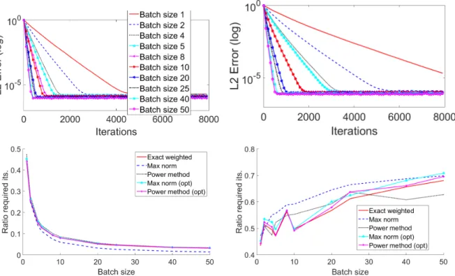
Noisy (inconsistent) systems: Lastly, we consider systems that are noisy, i.e. they have no exact solution. We seek convergence to the least squares solutionxLS. We consider the same Gaussian

matrix with variation as desribed above. We first generate a consistent systemAx=band then add a residual vectore tob that has norm one,kek2=1. Since the step size in (3.5) depends

on the magnitude of the residual, it will have to be estimated in practice. In our experiments, we estimate this term by an upper bound which is 1.1 times larger in magnitude than the true residualkAxLS−bk2. In addition, we choose an accuracy tolerance ofε=0.1. Not surprisingly,

our experiments in this case show similar behavior to those mentioned above, only the method convergences to a larger error (which can be lowered by adjusting the choice ofε). An example of such results in the correlated Gaussian case are shown in Figure 8.

Figure 1 (Gaussian linear systems: convergence)Mini-batch SGD on a Gaussian 1000_×50 system with var-ious batch sizes; batches created randomly at onset. Graphs show mean L2-error versus iterations (over 40 trials). Step sizeγused on each batch was as given in (3.5) for the weighted cases and as in [NSW16, Corollary 3.2] for the uniform comparisons, where in all cases corresponding approximations were used to compute the spectral norms. Left: Batches are selected using proposed weighted selection strategy (3.4). Right: Ratio of the number of iterations required to reach an error of 10−5for weighted batched SGD versus classical (sin-gle functional) uniform (unweighted) SGD. The notation “(opt)” signifies that the optimal step size was used, rather than the approximation.

Figure 2 (Gaussian linear systems with variation: convergence)Mini-batch SGD on a Gaussian 1000_×50

system whose entries in rowkhave variancek2, with various batch sizes. Graphs show mean L2-error

ver-sus iterations (over 40 trials). Step sizeγused on each batch was as given in (3.5) for weighted SGD and the optimal step size as in [NSW16, Corollary 3.2] for uniform sampling SGD. Left: Batches are created randomly at onset, then selected using weighted sampling. Center: Batches are created sequentially at onset, then se-lected using weighted sampling. Right: Batches are created sequentially at onset, then sese-lected using uniform (unweighted) sampling.

Figure 3 (Gaussian linear systems with variation: effect of weighting) Mini-batch SGD on a Gaussian

1000_×50 system whose entries in rowkhave variancek2, with various batch sizes; batches created

sequen-tially at onset. Step sizeγused on each batch was set as in (3.5) (approximations for Lipschitz constants also apply to the step size computation) for the weighted cases and as in [NSW16, Corollary 3.2] for the uniform cases. Left: Ratio of mean L2-error using weighted versus unweighted random batch selection (improvements appear when plot is less than one). Right: Ratio of the number of iterations required to reach an error of 10−5

for various weighted selections versus unweighted random selection. The notation “(opt)” signifies that the optimal step size was used, rather than the approximation.

Figure 4 (Gaussian linear systems with variation: effect of batching)Mini-batch SGD on a Gaussian 1000_×50 system whose entries in rowkhave variancek2, with various batch sizes; batches created sequentially at

on-set. Step sizeγused on each batch was set as in (3.5) (approximations for Lipschitz constants also apply to

the step size computation) for the weighted cases and as in [NSW16, Corollary 3.2] for the uniform cases. Left: Ratio of mean L2-error using weighted batched SGD versus classical (single functional) weighted SGD (improvements appear when plot is less than one). Right: Ratio of the number of iterations required to reach

an error of 10−5for various weighted selections with batched SGD versus classical (single functional)

uni-form (unweighted) SGD. The notation “(opt)” signifies that the optimal step size was used, rather than the approximation.

6. CONCLUSION

We have demonstrated that using a weighted sampling distribution along with batches of functionals in SGD can be viewed as complementary approaches to accelerating convergence. We analyzed the ben-efits of this combined framework for both smooth and non-smooth functionals, and outlined the specific convergence guarantees for the smooth least squares problem and the non-smooth hinge loss objective. We discussed several computationally efficient approaches to approximating the weights needed in the proposed sampling distributions and showed that one can still obtain approximately the same improved convergence rate. We confirmed our theoretical arguments with experimental evidence that highlight in

Figure 5 (Gaussian linear systems with variation: using power method)Mini-batch SGD on a Gaussian

1000×50 system whose entries in rowkhave variancek2, with various batch sizes; batches created

sequen-tially at onset. Step sizeγused on each batch was set as in (3.5) (approximations for Lipschitz constants also apply to the step size computation) for the weighted cases and as in [NSW16, Corollary 3.2] for the uniform cases. Lipschitz constants for batches are approximated by using²−1log(²−1b) (with²=0.01) iterations of the power method. Left: Convergence of the batched method. Next: Required number of computational flops to

achieve a specified accuracy as a function of batch size when computation is shared overbcores (center) or

done on a single node (right).

Figure 6 (Correlated systems with variation: convergence)Mini-batch SGD on a uniform 1000_×50 system

whose entries in rowkhave variancek2, with various batch sizes. Graphs show mean L2-error versus

itera-tions (over 40 trials). Step sizeγused on each batch was set as in (3.5) (approximations for Lipschitz constants also apply to the step size computation) for the weighted cases and as in [NSW16, Corollary 3.2] for the uni-form cases. Left: Batches are created randomly at onset, then selected using weighted sampling. Center: Batches are created sequentially at onset, then selected using weighted sampling. Right: Batches are created sequentially at onset, then selected using uniform (unweighted) sampling.

Figure 7 (Orthonormal, sparse, and tomography systems: convergence)Mini-batch SGD on two systems for various batch sizes; batches created randomly at onset. Graphs show mean L2-error versus iterations (over 40 trials). Step sizeγused on each batch was set as in (3.5). Left: Matrix is a 200×200 orthonormal discrete

Fourier transform (DFT). Center: 1000×50 matrix is a sparse standard normal matrix with density 20%. Right:

Tomography data (1200×400 system).

many important settings one can obtain significant acceleration, especially when batches can be com-puted in parallel. It will be interesting future work to optimize the batch size and other parameters when the parallel computing must be done asynchronously, or in other types of geometric architectures.

Figure 8 (Noisy systems: convergence)Mini-batch SGD on a Gaussian 1000_×50 system whose entries in row

k have variancek2, with various batch sizes. Noise of norm 1 is added to system to create an inconsistent

system. Graphs show mean L2-error versus iterations (over 40 trials). Step sizeγused on each batch was set

as in (3.5) for the weighted case and as in [NSW16, Corollary 3.2] for the uniform case; the residualAxLS−b

was upper bounded by a factor of 1.1 in all cases. Upper Left: Batches are created sequentially at onset, then selected using weighted sampling. Upper Right: Batches are created sequentially at onset, then selected using uniform (unweighted) sampling. Lower Left: Ratio of the number of iterations required to reach an

error of 10−5for various weighted selections with batched SGD versus classical (single functional) uniform

(unweighted) SGD. Lower Right: Ratio of the number of iterations required to reach an error of 10−5for various weighted selections with batched SGD versus classical uniform (unweighted) SGD as a function of batch size.

ACKNOWLEDGEMENTS

The authors would like to thank Anna Ma for helpful discussions about this paper. Needell was par-tially supported by NSF CAREER grant #1348721 and the Alfred P. Sloan Foundation. Ward was parpar-tially supported by NSF CAREER grant #1255631.

REFERENCES

[AD11] A. Agarwal and J. C. Duchi. Distributed delayed stochastic optimization. InAdvances in Neural Information Pro-cessing Systems, pages 873–881, 2011.

[BB11] L. Bottou and O. Bousquet. The tradeoffs of large-scale learning.Optimization for Machine Learning, page 351, 2011.

[BCNW12] R. H. Byrd, G. M. Chin, J. Nocedal, and Y. Wu. Sample size selection in optimization methods for machine learning.

Mathematical programming, 134(1):127–155, 2012.

[BM11] F. Bach and E. Moulines. Non-asymptotic analysis of stochastic approximation algorithms for machine learning.

Advances in Neural Information Processing Systems (NIPS), 2011.

[Bot10] L. Bottou. Large-scale machine learning with stochastic gradient descent. InProceedings of COMPSTAT’2010, pages 177–186. Springer, 2010.

[CQR15] D. Csiba, Z. Qu, and P. Richtarik. Stochastic dual coordinate ascent with adaptive probabilities.Proceedings of the 32nd International Conference on Machine Learning (ICML-15), 2015.

[CSSS11] A. Cotter, O. Shamir, N. Srebro, and K. Sridharan. Better mini-batch algorithms via accelerated gradient methods. InAdvances in neural information processing systems, pages 1647–1655, 2011.

[CT05] E. J. Candès and T. Tao. Decoding by linear programming.IEEE T. Inform. Theory, 51:4203–4215, 2005.

[DB15] A. Défossez and F. R. Bach. Averaged least-mean-squares: Bias-variance trade-offs and optimal sampling distribu-tions. InAISTATS, 2015.

[DGBSX12] O. Dekel, R. Gilad-Bachrach, O. Shamir, and L. Xiao. Optimal distributed online prediction using mini-batches.The Journal of Machine Learning Research, 13(1):165–202, 2012.

[GR16] R. M. Gower and P. Richtárik. Randomized quasi-newton updates are linearly convergent matrix inversion algo-rithms.arXiv preprint arXiv:1602.01768, 2016.

[Han07] P. C. Hansen. Regularization tools version 4.0 for matlab 7.3.Numer. Algorithms, 46(2):189–194, 2007.

[KL96] P. Klein and H.-I. Lu. Efficient approximation algorithms for semidefinite programs arising from max cut and col-oring. InProceedings of the twenty-eighth annual ACM symposium on Theory of computing, pages 338–347. ACM, 1996.

[KLRT16] J. Konecn`y, J. Liu, P. Richtarik, and M. Takac. ms2gd: Mini-batch semi-stochastic gradient descent in the proximal setting.IEEE Journal of Selected Topics in Signal Processing, 10(2):242–255, 2016.

[LS13] Y. T. Lee and A. Sidford. Efficient accelerated coordinate descent methods and faster algorithms for solving linear systems. InFoundations of Computer Science (FOCS), 2013 IEEE 54th Annual Symposium on, pages 147–156. IEEE, 2013.

[LZCS14] M. Li, T. Zhang, Y. Chen, and A. J. Smola. Efficient mini-batch training for stochastic optimization. InProceedings of the 20th ACM SIGKDD international conference on Knowledge discovery and data mining, pages 661–670. ACM, 2014.

[Nee10] D. Needell. Randomized Kaczmarz solver for noisy linear systems.BIT, 50(2):395–403, 2010. [Nes04] Y. Nesterov.Introductory Lectures on Convex Optimization. Kluwer, 2004.

[Nes12] Y. Nesterov. Efficiency of coordinate descent methods on huge-scale optimization problems.SIAM J. Optimiz., 22(2):341–362, 2012.

[NJLS09] A. Nemirovski, A. Juditsky, G. Lan, and A. Shapiro. Robust stochastic approximation approach to stochastic pro-gramming.SIAM Journal on Optimization, 19(4):1574–1609, 2009.

[NSW16] D. Needell, N. Srebro, and R. Ward. Stochastic gradient descent and the randomized kaczmarz algorithm. Mathe-matical Programming Series A, 155(1):549–573, 2016.

[NW13] D. Needell and R. Ward. Two-subspace projection method for coherent overdetermined linear systems.Journal of Fourier Analysis and Applications, 19(2):256–269, 2013.

[QRZ15] Z. Qu, P. Richtarik, and T. Zhang. Quartz: Randomized dual coordinate ascent with arbitrary sampling. InAdvances in neural information processing systems, volume 28, pages 865–873, 2015.

[RM51] H. Robbins and S. Monroe. A stochastic approximation method.Ann. Math. Statist., 22:400–407, 1951.

[RSS12] A. Rakhlin, O. Shamir, and K. Sridharan. Making gradient descent optimal for strongly convex stochastic optimiza-tion.arXiv preprint arXiv:1109.5647, 2012.

[RT15] P. Richtárik and M. Takáˇc. On optimal probabilities in stochastic coordinate descent methods.Optimization Letters, pages 1–11, 2015.

[SRB13] M. Schmidt, N. Roux, and F. Bach. Minimizing finite sums with the stochastic average gradient.arXiv preprint arXiv:1309.2388, 2013.

[SSS08] S. Shalev-Shwartz and N. Srebro. SVM optimization: inverse dependence on training set size. InProceedings of the 25th international conference on Machine learning, pages 928–935, 2008.

[SSSSC11] S. Shalev-Shwartz, Y. Singer, N. Srebro, and A. Cotter. Pegasos: Primal estimated sub-gradient solver for svm. Math-ematical programming, 127(1):3–30, 2011.

[SV09] T. Strohmer and R. Vershynin. A randomized Kaczmarz algorithm with exponential convergence.J. Fourier Anal. Appl., 15(2):262–278, 2009.

[SZ12] O. Shamir and T. Zhang. Stochastic gradient descent for non-smooth optimization: Convergence results and opti-mal averaging schemes.arXiv preprint arXiv:1212.1824, 2012.

[TBRS13] M. Takac, A. Bijral, P. Richtarik, and N. Srebro. Mini-batch primal and dual methods for SVMs. InProceedings of the 30th International Conference on Machine Learning (ICML-13), volume 3, pages 1022–1030, 2013.

[XZ14] L. Xiao and T. Zhang. A proximal stochastic gradient method with progressive variance reduction.SIAM Journal on Optimization, 24(4):2057–2075, 2014.

[YCRM16] J. Yang, Y.-L. Chow, C. Ré, and M. W. Mahoney. Weighted sgd for`pregression with randomized preconditioning. InProceedings of the Twenty-Seventh Annual ACM-SIAM Symposium on Discrete Algorithms, pages 558–569. SIAM, 2016.

[ZZ15] P. Zhao and T. Zhang. Stochastic optimization with importance sampling for regularized loss minimization. In Pro-ceedings of the 32nd International Conference on Machine Learning (ICML-15), 2015.