On Maximum Likelihood Estimators of the Parameters of a Modified Weibull Distribution Using Extreme Ranked Set Sampling

(1)

Methods

Volume 10 | Issue 2

Article 18

11-1-2011

On Maximum Likelihood Estimators of the

Parameters of a Modified Weibull Distribution

Using Extreme Ranked Set Sampling

Amer Ibrahim Al-Omari

Al al-Bayt University, [email protected]

Said Ali Al-Hadhrami

College of Applied Sciences, [email protected]

Follow this and additional works at:

http://digitalcommons.wayne.edu/jmasm

Part of the

Applied Statistics Commons,

Social and Behavioral Sciences Commons, and the

Statistical Theory Commons

This Regular Article is brought to you for free and open access by the Open Access Journals at DigitalCommons@WayneState. It has been accepted for inclusion in Journal of Modern Applied Statistical Methods by an authorized administrator of DigitalCommons@WayneState.

Recommended Citation

Al-Omari, Amer Ibrahim and Al-Hadhrami, Said Ali (2011) "On Maximum Likelihood Estimators of the Parameters of a Modified Weibull Distribution Using Extreme Ranked Set Sampling,"Journal of Modern Applied Statistical Methods: Vol. 10: Iss. 2, Article 18. Available at:http://digitalcommons.wayne.edu/jmasm/vol10/iss2/18

(2)

607 On Maximum Likelihood Estimators of the Parameters of a Modified

Weibull Distribution Using Extreme Ranked Set Sampling

Amer Ibrahim Al-Omari

Said Ali Al-Hadhrami

Al al-Bayt University,

Mafraq, Jordan

College of Applied Sciences, Nizwa, Oman

Extreme ranked set sampling (ERSS) is considered to estimate the three parameters and population mean of the modified Weibull distribution (MWD). The maximum likelihood estimator (MLE) is investigated and compared to the corresponding one based on simple random sampling (SRS). It is found that, the MLE based on ERSS is more efficient than MLE using SRS for estimating the three parameters of the MWD. The ERSS estimator of the population mean of the MWD is also found to be more efficient than the SRS based on the same number of measured units.

Key words: Modified Weibull distribution, extreme ranked set sampling, maximum likelihood estimator, simple random sampling, information number.

Introduction

The modified Weibull distribution (MWD) was suggested by Sarhan and Zaindin (2009). The probability density function (pdf) of the MWD is given by

(

)

(

1

) (

)

; , , exp , 0, f x x x x x γ γ

α β γ

α βγ

−

α

β

= + − − > (1) and the corresponding distribution function (cdf) is

(

; , ,

)

1 exp

(

)

, 0,

F x

α β γ

= − −

α

x−

β

xγ x>

(2) where

γ

>

0

and

α

,

β

≥0 such that

Amer Ibrahim Al-Omari is an Assistant Professor in the Department of Mathematics.

Email him at: [email protected]. Said

Ali Al-Hadhrami is an Assistant Professor in the Department of Mathematics, College of Applied Sciences. Email him at: [email protected].

0

α β

+ > . The MWD have two shape

parameters

γ

and

β

, and a scale parameter

α

. The hazard function of the MWD is

(

_{; , ,}

)

1

h x

_{α β γ}

_{= +}

_{α βγ}

x

γ− _{, (3)} which increases for

γ

>1, decreases for

γ

<1

and remains constant for

γ

=1. Sarhan and Zaindin (2009) defined the kth_moment,

k

μ

, of the MWD random variable as

( )

(

)

(

)

(

)

(

)

0 /

1 !

,

0,

/

1 0,

0,

1 0,

0.

i i k i k i k k k

i

k

i

k

i

if

k

if

k

if

γ γ γ γ

β

γ

βγ γ γ

α

α β

μ

_γ

α

β

α

β

∞ + + + =



₋

_

_Γ

_{+ +}

_Γ

_{+ +}

_

+



_

_









_>



=



_Γ

₊

=

>



_{Γ +}

>

=







(4) The moment generating function of the MWD is given by

(3)

608 ( )

(

)

(

)

(

)

1 0 / 0 1 ! ( ) ( ) , 0, , ( ) _/ ₁ 0, 0, 0, 0, . i i i i i i i i i i t t if t M t _t _i if if t t γ γ γ γ β α γ βγ γ γ α α α β α γ _α _β β α _α _β _α α ∞ + + = ∞ =  ₋ _ _Γ ₊ _Γ ₊ _ +    − −     _> _>  = _Γ ₊  ₌ _>    > = > − 



(5) Some special cases of the MWD distribution are the exponential distribution, Raleigh distribution, linear failure rate distribution and Weibull distribution. For additional details about the MWD see: Sarhan & Zaindin (2009) and Zaindin & Sarhan (2009). The maximum likelihood estimator of the three parameters and the population mean of the modified Weibull distribution is examined, and compared to their counterparts based on simple random sampling. The MLE of the parameters based on ERSS is considered for two cases: when the set size is even and odd.

RSS and ERSS

Ranked set sampling (RSS) was proposed by McIntyre (1952) to improve the estimation of the population mean. The following steps are employed to obtain an RSS of size m:

Step 1: Randomly select _m2_{units from the}

population; these units are randomly allocated into m sets, each of size m. Step2: The m units of each set are ranked either

visually or by any inexpensive method with respect to the variable of interest. Step3: From the first set of m units, the smallest

ranked unit is measured; from the second set of m units the second smallest ranked unit is measured. The process continued until the mth_smallest

unit (largest) is measured from the last set.

Step 4: The procedure can be repeated n times if needed to increase the sample size to nm

units.

It should be noted that the error in ranking reduces the efficiency of the method. Extreme ranked set sampling was proposed by Samawi, et al. (1996) as a useful modification of RSS. It requires identifying the extreme units only, as opposed to all ranks as in the usual RSS. The method gives an unbiased estimate of the population mean in the case of symmetric distributions and it is more efficient than SRS.

The extreme ranked set sampling (ERSS) method can be described as follows: Step 1: Select m random samples each of size m

units from the target population.

Step 2: Rank the units within each sample with respect to a variable of interest by visual inspection or any other inexpensive method.

Step 3: For actual measurement, if the sample size m is even, from the first

2

m

sets select the lowest ranked unit of each set and from the other

2

m

sets select the largest ranked unit. If the sample size is odd, from the first 1

2

m− _{sets select the}

lowest ranked unit, from the other

1 2

m− _{sets select the largest ranked unit,}

and from the remaining set the median ranked unit is selected.

Step 4: The procedure can be repeated n times if needed to increase the sample size to nm

units.

Let

X

₁,

X

₂

...

,

X

_m be a simple random sample from the probability density function f x( ), with mean

μ

and variance

_σ

2_.

(4)

609

1

m

X

,

X

_m₂,

...,

X

_mm be m independent SRS each of size m. Let X_i₍₁₎,X_i₍₂₎,

...

, X_{i m}_{( )} be the order statistics of the sample

X

_i₁,

X

_i₂,

...,

im

X

for

(

i

₌

1, 2,...,

m

)

. The pdf and cdf of the

ith_{order statistics,} ( )i X , respectively are

[

] [

1

]

( ) ! ( ) ( ) 1 ( ) ( ), ( 1)!( )! i m i i m f x F x F x f x i m i − − = − − − and

( ) (

)

( ) 1 ( ) 0

!

( )

(1

)

1 !

!

F x i m i i

m

F x

v

dv

i

m i

− −

=

−



.

The mean and the variance of X_{( )}_i are given by

( )i

xf

( )i

( )

x dx

μ

∞ −∞

=



and

(

)

2 2 ( )i

x

( )i

f

( )i

( )

x dx

σ

∞

μ

−∞

=



−

,

respectively (see David and Nagaraja, 2003). Takahasi and Wakimoto (1968) provided the mathematical properties of the RSS and gave the following identities ( ) 1 1 ( ) ( ) m i i f x f x m = =



, _{( )} 1 1 m i i m

μ

= =



, and

(

)

2

(

)

2 ( ) 2 1

1 ˆ

Var

_RSS m _i i

m

σ

μ

=

−



−

. They showed that the efficiency of RSS with respect to SRS is

(

ˆ ˆ

)

Var

(

₍

ˆ

)

₎

1 1 , ˆ Var 2 SRS RSS SRS RSS m eff

_μ

μ

+ ≤ = ≤ ,

where

μ

ˆ

_SRS and

μ

ˆ

_RSS are unbiased estimators of the population mean

μ

using SRS and RSS, respectively.

When m is even, the ERSS estimator of the population mean is defined as

/ 2 1 ( ) , (1) , 1 1 / 2 1

1 ˆ

_ERSS r m _{m i j} m _{i j} j i i m

X

rm

μ

= = = +





=

_

+

_





 



, (6) and when m is odd

( ) ( 1)/2 1 ( ) , (1) , 1 ( 1)/2 2 1 ( 1)/2 ,

1 ˆ

,

m m r m i j i j i i m ERSS j m i j

X

rm

X

μ

− − = = + = +





+





=







₊









(7) where X_{( ) ,}_{k i j} denotes the kth ranked from the ith

set at the jth cycle.

Samawi, et al. (1996) showed that the sample mean using ERSS is more efficient than that of SRS when the distribution is symmetric. Samawi and Al-Sagheer (2001) investigated the ERSS method to estimate the distribution function and Muttlak (2001) considered regression estimation using extreme and median ranked set samples methods. Samawi and Saeid (2004) studied the stratified ERSS and the ratio estimator based on ERSS. Al-Omari, et al. (2008) considered ratio type estimator based on ERSS. For more about RSS and its modifications see: Arnold, et al. (2009); Al-Omari & Jaber (2008); Bouza (2009); Shadid, et al. (2011); Al-Hadhrami & Al-Omari (2009); Islam, et al. (2009); Jemain & Al-Omari (2006); Sengupta & Mukhuti (2009).

Maximum Likelihood Estimation of the MWD: When m is Even

The maximum likelihood estimators (MLEs) of the three estimators

α

,

β

and

γ

when m is even are investigated based on the likelihood function L using ERSS as

(

) (

)

{

}

(

)

(

)

{

}

1 ( ) , ( ) , 1 1 1 (1) , (1) , 1 1 , 1 p r _m m i j m i j i j r m _m i j i j i j p h mf x F x L mf x F x − = = − = = +  _ _   _ _    =_ _   × −        

∏∏

∏ ∏

(8)

(5)

610

where p m= / 2 and h is a constant. The variable X_{( ) ,}_{k i j} denotes the kth_{ranked unit of the}

ith sample at the jth cycle. The log likelihood function of (8) is

(

)

(

)

(

)

(

)

(

)

* ( ) , 1 1 ( ) , 1 1 (1) , 1 1 (1) , 1 1

ln

(

1)

ln

+

ln

(

1)

ln 1

,

p r m i j j i p r m i j j i r m i j j i p r m i j j i p

L

C

f x

m

F x

f x

m

F x

= = = = = = + = = +

= +

+

−

+

−



 

(9) where C is a constant. The first derivatives of

*

L

with respect to

α

,

β

and

γ

, respectively are * ( ) , 1 1 1 ( ) , ( ) , 1 1 1 1 (1) , 1 1 (1) , 1 1 1 (1) , 1 ( 1) 1 ( 1) 1 + , p r m i j j i m i j p r m i j j i r m i j j i p r m i j j i p i j L x x x T m T m x x x γ γ

α

α βγ

− = = = = = = + − = = +   ∂ = _ − _ ∂ _ + _   + −   −   − −   −    ₊   



 

(10) 1 * ( ) , ( ) , 1 1 1 ( ) , ( ) , 1 1 1 1 (1) , 1 1 1 (1) , (1) , 1 1 1 (1) , ( 1) 1 ( 1) p r m i j m i j j i m i j p r m i j j i r m i j j i p r m i j i j j i p i j x L x x x T m T m x x x x γ γ γ γ γ γ γ γ

γ

β

α βγ

γ

α βγ

− − = = = = = = + − − = = +   ∂ = _ − _ ∂ _ + _   + − _ _ −   − −   + _ − _ +  



 



,



(11)

(

)

(

)

(

)

(

)

(

)

(

)

(

)

1 ( ) , ( ) , * 1 ( ) , 1 1 ( ) , ( ) , 1 (1) , (1) , 1 (1) , 1 1 (1) , (1) , ( ) , ( ) , ln 1 ln ln 1 + ln ln ( 1) m i j m i j p r m i j j i m i j m i j i j i j r m i j j i p i j i j m i j m i j x x L x x x x x x x x x x T m γ γ γ γ γ γ γ

β

γ

α βγ

γ

β

γ

α βγ

β

− − = = − − = = +  ₊    ∂ ₌ _ ₊ _ ∂   ₋     ₊     +    ₋    + −



 

(

)

1 1 1 1 (1) , (1) , 1 1 1 _, ( 1) ln p r r m j i i j i j j i p T m

_β

x xγ = = = = +     −     _{− −}     



 

(12) where

(

1

)

1 exp ( ) ,m i j ( ) ,m i j T ₌ ₋

_α

x ₋

_β

xγ− and

(

)

2 exp (1) ,i j (1) ,i j T = −

α

x −

β

xγ .

The MLE of the parameters

α β

, , and

γ

are the solution of equations (10), (11) and (12), respectively, when set them to zero. However, the solutions are not in closed forms, in order to obtain estimates for the parameters, the three equations may be solved numerically.

Fisher information (FI) numbers describe the amount of information that a sample provides about the parameters. The FI is defined as 2 2

log( )

L

I

E

θ



_∂



= −





∂





,

where

θ

is a parameter. The FI number from ERSS for estimating

α

,

β

and

γ

can be expressed as in equations, (13), (14) and (15), respectively as

(6)

611 (

)

(

)

( )

₍

₎

2 ( ) , 1 2 1 1 1 _{( ) ,} 1 1 1 2 ( ) , 1 2 ₁ 2 1 1 ₁ 1 1 (1) , ( ) 1 ( 1) 1 1 ( 1) , 1 ERSS p p r r m i j j i _{m i j} j i p r r m m i j j i j i p i j I x T E m T x x T m T x γ γ α α βγ α βγ − = = = = − = = = = + =   ₋  _₋ _  _ _ −  _ _+ − _ _ − +  _ _         ₋ _     − − _ _+ _ _  − +      



 

(13)

(

)

2 1 ( ) , 1 1 1 ( ) , 2 1 (1) , 1 1 1 (1) , 2 2 ( ) , 1 ( ) , 1 1 1 1 1

( )

(

1)

,

1

p r m i j ERSS j i m i j r m i j j i p i j p r m i j m i j j i

x

I

E

x

T

x

T

m

T

γ γ γ γ γ γ

γ

β

α βγ

γ

α βγ

− − = = − − = = + = =



_

_



= −



−





+

















−





+













_

_{ }







− −

_

+



_

 

_

_

−

_

−

_

_







 



(14) and

(

)

(

)

(

)

(

)

(

)

(

)

(

)

2 ( ) , 2 2 1 1 ( ) , 2 2 (1) , 2 2 1 1 (1) , 2

( )

log

(

1)

log

,

(

1)

log 1

ERSS m i j p r j i m i j i j p r j i i j

I

f x

E

m

F x

f x

m

F x

β

γ

= = = =

=





_∂







_∂





_

_

−



_

_

∂



_

₊

₋

_



_

_∂

_







_∂







_∂



_





−

_

_



∂

_

_



+

−



_

_{ }



∂







(15) where

( )

(

)

(

)

(

)

(

)

2 (.) , 2 1 ( ) , ( ) , ( ) , 1 ( ) , 2 1 ( ) , ( ) , 1 ( ) , 2 , ( ) , log ln ln 2 ln 1 ln , i j m i j m i j m i j m i j m i j m i j m i j i j m i j f x x x x x x x x x x γ γ γ γ γ

γ

β

γ

α βγ

β

γ

α βγ

β

− − − − ∂ _ _₌   ∂    ₊      +   ₊     −  +     −

( )

(

)

( )

2 (.) , 2 2 2 (.) , (.) , (.) , 2 2 (.) , (.) , 1 1 log ln 1 1 ln 1 i j i j i j i j i j i j F x T x x x T x x T T γ γ γ γ β β β ∂ _ _₌   ∂ − −   −  −     and

( )

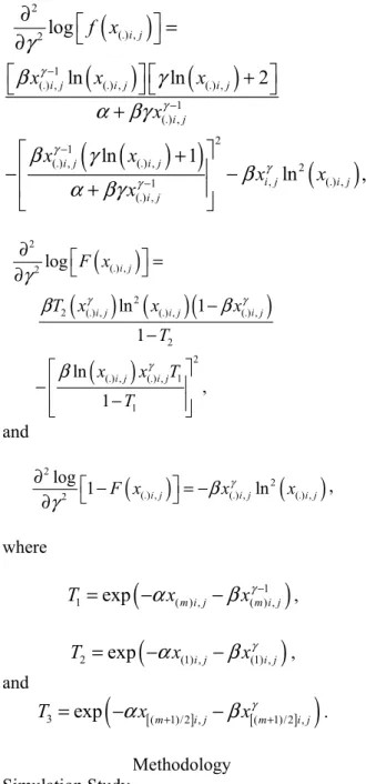
2 2 (.) , (.) , (.) , 2log 1 F x i j βxγi jln x i j γ ∂ _ ₋ __{= −}   ∂ .

Maximum Likelihood Estimation of the MWD: When m is Odd

Based on ERSS, when m is odd, the likelihood function is

(

) (

)

{

}

(

)

(

)

{

}

(

) (

)

(

)

1 ( ) , ( ) , 1 ₁ 1 1 (1) , (1) , 1 1 1 2 (( 1)/2) (( 1)/2) (( 1)/2)

1

m m i j m i j q r r m _m i j i j i j i j q m m j m j m j

mf x

F x

L K

mf x

F x

f x

F x

− − ₋ = = = = + − + + +



_

_















=



_

₋

_

















₋







∏∏

∏ ∏

(16) where q =(m−1) / 2 and K is a constant. The log likelihood function of (16) is

(7)

612 (

)

(

)

(

)

(

)

{

}

( )

( ) (

)

1 2 1 1 2 2 * * ( ) , 1 1 ( ) , 1 1 1 ( ) , 1 1 1 (1) , 1 1 ( ) ( ) ( )

( )

ln

(

1)

ln

(

1)

ln 1

log

1 log

log 1

(

.

2

m m m q r m i j j i q r m i j j i r m m i j j i q r m i j j i q j j j

L

Ln L

K

f x

m

F x

f x

m

F x

f x

m

F x

+ + + = = = = − = = + − = = +

=

+





+

−

_

_

+





+

−

_

−

_

+

−

_

_

+

_

_

+

−

_

_



 

(17) Taking the first derivative of

_L

*_{in (17) with}

respect to

α β

, and

γ

results in

* ( ) , 1 1 1 ( ) , 1 ( ) , 1 1 1 ( ) , 1 ( ) , 1 1 1 1 1 (1) , 1 1 1 ₍ 1 ( ) 2 1 1 1 1 +( 1) ( 1) q r m i j j i m i j r m m i j j i q m i j r m m i j j i r m i j j i q m _j x L x x x x x T m T m x x γ γ γ

α βγ

α

α βγ

− = = − − = = + − = = − = = + − + − − − −   ∂ = _ _ + ∂ _ _   + _ _ +   − − − + +



 



 

1₎ 1 2 1 3 ( ) 2 1 ( ) 1 1 3 2 1 , 2 r m _j j r m _j m j j x T m x T + = + + = − −             − _ _ + _ _  



(18) 1 * ( ) , ( ) , 1 1 1 ( ) , 1 1 (1) , (1) , 1 1 1 (1) , 1 ( ) , 1 (1) , 1 1 1 1 1

(

1)

(

1)

1

q r m i j m i j j i m i j r m i j i j j i q i j q r r m m i j i j j i j i q

x

L

x

T

m

x

T

γ γ γ γ γ γ γ γ

γ

β

α βγ

γ

α βγ

− − = = − − − = = + − = = = = +





∂ =



_

−



_

∂

_

+

_





+



_

−



_

+









+

−



_



_

−







 



 

1 2 1 2 1 2 1 2 1 2 1 ( ) 1 ( ) 1 ₍ ₎ 3 ( ) ( ) 1 3

1 ,

2

1

m m m m m r j j j _j r j j j

x

T

m

x

T

γ γ γ γ γ

γ

α βγ

+ + + + + − − = =









+

_

−

_

+









−

_

_

+

_

−

_

−







(19) and

(

)

(

)

(

)

(

)

1 ( ) , * 1 ( ) , 1 1 ( ) , ( ) , 1 (1) , 1 1 (1) , 1 1 (1) , (1) , ( ( ) , (1) , ln + ln ln ( 1) ln 1 ln 1 m i j q r m i j j i m i j m i j i j r m i j j i q i j i j m i j i j x L x x x x x x x x m x x γ γ γ γ γ γ β α βγ γ β β α βγ β β

γ

− − = = − − − = = + ∂ = + ∂ − + − + −  _ ₊ _            _ ₊ _          



 

(

)

(

)

( )

1 2 1 2 ) , ( ) , 1 1 1 1 ( 1) , ( 1) , 1 1 1 1 ( ) 2 1 ( ) 1 1 1 ( ) ( ) 2 2 1 ( ) , 2 ( ) 1 ( 1) ln ln ln 1 2 ln 1 m m q r m i j m i j j i q r p i j p i j j i m _j r j j m _j m _j m _{i j} j x T T m x x x x x x x m x γ γ γ γ γ β β α βγ β β

γ

+ + = = + + = = − + − = + + + − − − + + − − +         ₊            _ _   _ _     





1 3 ( ) , 2 3 1 1 1 ( ) , ( ) , 2 2 1 , ln m _{i j} r j m _{i j} m _{i j} x T T x x γ γ β + = + + − −        _ _       _ _         



(20)

(8)

613

respectively, where

(

1

)

1 exp ( ) ,m i j ( ) ,m i j T ₌ ₋

_α

x ₋

_β

xγ− _,

(

)

2 exp (1) ,i j (1) ,i j T ₌ ₋

_α

x ₋

_β

xγ and

(

)

3 exp ((m 1)/2) ,i j ((m 1)/2) ,i j T

_α

x

_β

xγ + + = − − .

The Fisher Information number of

α β

,

and

γ

from the samples, respectively are

(

)

(

)

(

)

(

)

2 1 1 1 _{( ) ,} 2 2 ( ) , 1 ( ) , 1 2 1 1 1 ₁ 1 2 1 1 1 (1) , 2 1 ₁ 1 ( ) 2 2 1 3 1 3 ( ) ( ) 2 2 3 3

1 ( )

(

1)

1

2

1

q r ERSS j i _{m i j} q r m i j m i j j i r m j i q i j r j m j m _j m _j

I

E

x

T

x

T

m

T

x

T

x

T

m

T

γ γ γ

α

α βγ

− = = = = − − = = + = ₋ + + +



₋



= −



+











−

_

+

_

−





−

+

−

+





+













−



−

+

_

−

_

−





 



2 1

,

r j=











_







_{ }





_









(21)

(

)

(

)

(

)

(

)

(

)

2 1 ( ) , 2 1 1 1 _{( ) ,} 2 1 1 (1) , 2 1 1 1 _{(1) ,} 2 2 ( ) , 1 ( ) , 1 1 1 1 1 1 1 ( ) 2 1 ( 2 ( ) + ( 1) 1 1 q r m i j ERSS j i _{m i j} r m i j j i q _{i j} q r m i j m i j j i m _j m x I E x x x x T x T m T T x x γ γ γ γ γ γ γ

γ

β

α βγ

γ

α βγ

γ

α βγ

− − = = − − − = = + = = − + +   ₋   _ _ = −  _ _ +  _ _   ₋     ₊     _ _    − − _ +_ _ _ − _ − _   − +



 



2 1 1 ) 2 2 1 3 1 3 ( ) ( ) 2 2 1 3 3 1 , 2 1 1 r j j m m r j j j x T x T m T T γ γ γ − = + + =            _ _   _ _     −      − _ +_ _ _ − _ − _ _  _       



(22)

(

)

(

)

(

)

(

)

2 ( ) , 2 2 1 1 ( ) , 2 2 (1) , 2 2 1 1 (1) , 2 2 1 2 ₍ _{) ,} 2 1

( )

log

+(

1)

log

(

1)

log 1

log

1

2

ERSS m i j q r j i m i j i j q r j i i j r m _{i j} j

I

f x

E

m

F x

f x

m

F x

f x

m

γ

= = = = + =

=





_∂

_

_







_∂

_

_





_

_

−



_

_

∂



_

₋

_

_

_







_

_∂

_





_∂

_

_





_∂

_

_







+

_

_

∂

_

_

+

−



_

_



∂









∂





+

_

_

_

_

∂









−

+





2 1 2 ₍ _{) ,} 2 1 2 1 2 ₍ _{) ,} 2

log

log 1

,

r m _{i j} j m _{i j}

F x

γ

+ = +





∂













∂















∂





+

_∂



−



_



_











(23) where

(9)

614 ( )

( )

(

)

_{( )}

2 (.) , 2 1 (.) , (.) , (.) , 1 (.) , 2 1 (.) , (.) , ₂ , (.) , 1 (.) , log ln ln 2 ln 1 ln , i j i j i j i j i j i j i j i j i j i j f x x x x x x x x x x γ γ γ γ γ

γ

β

γ

α βγ

β

γ

β

α βγ

− − − − ∂ _ _₌   ∂    ₊      +  ₊    − −  +   

( )

( ) ( )(

)

( )

2 (.) , 2 2 2 (.) , (.) , (.) , 2 2 (.) , (.) , 1 1 log ln 1 1 ln , 1 i j i j i j i j i j i j F x T x x x T x x T T γ γ γ γ β β β ∂ _ _₌   ∂ − −   −  −     and

( )

2 2 (.) , (.) , (.) , 2 log 1 F x i j βxγi jln x i j γ ∂ _ ₋ __{= −}   ∂ , where

(

1

)

1 exp ( ) ,m i j ( ) ,m i j T ₌ ₋

_α

x ₋

_β

xγ− _,

(

)

2 exp (1) ,i j (1) ,i j T = −

_α

x −

_β

xγ , and [ ] [ ]

(

)

3

exp

(m 1)/2 ,i j (m 1)/2 ,i j

T

=

−

_α

x

₊

−

_β

x

γ ₊ . Methodology Simulation Study

To investigate the properties of the MLEs of the three parameters of the MWD a simulation was conducted. The inverse transform method was used to generate samples from MWD (see Ros, 1997). The inverse transform algorithm can be described as: generate

U

from the uniform (0, 1), initiate

X

₁

and then find a new

X

₁ using

(

)

1 1 1 ln 1 X

β

Xγ U

α

= − − − ; repeat until stability of

X

₁ is reached, which eventually

represents a random number from MWD. The samples generated are then used to obtain the Fisher Information numbers,

I

_ERSS and

I

_SRS, when using ERSS and SRS. The asymptotic relative efficiency (RP) is found as the ratio

/

ERSS SRS

I

.

Results

For

_α

₌

3

,

β

=1.2 and

γ

=1.3, the results are presented in Tables 1, 2 and 3, respectively.

Table 1: Information Numbers and Asymptotic RP of the MLE of

α

Based on ERSS with respect to SRS

m

I

ERSS

I

SRS Asymptotic RP 3 0.3613 0.1854 1.9490 4 0.6069 0.2392 2.5372 5 0.7933 0.2849 2.7845 6 0.9818 0.3478 2.8229 7 1.3030 0.4057 3.2119 Table (2): Information Numbers and Asymptotic RP of

the MLE of

β

m

I

ERSS

I

the MLE of

γ

based on ERSS with respect to SRS

m

I

ERSS

I

SRS Asymptotic RP 3 0.6451 0.5348 1.2062 4 1.1279 0.8684 1.2987 5 1.2494 0.7336 1.7032 6 1.7856 0.9847 1.8133 7 1.9196 0.8459 2.2693

(10)

615

For

_α

₌

2.3

,

β

=1.3 and

γ

=1.6, results are summarized in Tables 4, 5 and 6 respectively.

Tables 1-3 show that:

• The ERSS estimators dominate the estimators based on SRS.

• The information numbers from ERSS are greater than those of SRS.

• For odd and even sample sizes the Fisher information numbers are increasing when the sample size is increasing.

• The asymptotic relative precision values are increasing when sample size increasing. Estimation of the Population Mean of the MWD

The problem of estimating the population mean of the MWD is now considered and compared with the SRS estimator of the population mean 1 ˆSRS m i/ i X m

μ

= =



, which has variance

_σ

2_/_m_{. The efficiency of}

1

ˆ

_ERSS

μ

and

2

ˆ

_ERSS

μ

respectively with respect to

_μ

ˆ

_SRS are defined as

(

ˆ

,

ˆ

)

₍

(

ˆ

)

₎

ˆ

SRS ERSSi SRS ERSSi

MSE

eff

MSE

μ

=

, i =1, 2.

Simulation results are summarized in Tables 7-9 for some values of the population parameters.

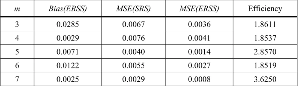
From results shows in Tables 7-9, it may be concluded that the ERSS estimators are biased and more efficient than the SRS estimator for all cases considered in this study. However, as demonstrated by Samawi, et al. (1996) it is better to use ERSS with small sample size. Also note that the efficiency of the mean estimation depends on the values of

α β

, ,

γ

, as well as the sample size.

Conclusion

Maximum likelihood estimators for the three parameters of the modified Weibull distribution were studied based on extreme ranked set sampling. These MLEs are not in closed forms, so numerical method is used. Results show that the Fisher information numbers obtained from ERSS are greater than that from SRS. Also, it was shown that ERSS is more efficient than SRS in estimating the population mean and it has a small bias. However, the ERSS estimators dominate the corresponding estimators based on SRS for estimating the population mean of the MWD.

Table (4): Information Numbers and Asymptotic RP of the MLE of

α

_{Based on ERSS with respect to SRS}

m

I

ERSS

I

the MLE of

β

m

I

ERSS

I

the MLE of

γ

m

I

ERSS

I

SRS Asymptotic RP 3 1.2459 0.7885 1.5801 4 1.9567 1.0232 1.9123 5 2.9202 1.3510 2.1615 6 3.8283 1.5697 2.4388 7 5.0158 1.7128 2.9284

(11)

616

References

Al-Hadhrami, S., & Al-Omari, A. I. (2009). Bayesian inference on the variance of normal distribution using moving extremes ranked set sampling. Journal of Modern Applied Statistical Methods, 8(1), 227-235.

Al-Omari, A. I., Jaber, K., & Al-Omari, A. (2008). Modified ratio type estimators of the mean using ranked set sampling. Journal of Mathematics and Statistics, 4(3), 150-155.

Al-Omari, A. I., & Jaber, K. (2008). Percentile double ranked set sampling. Journal of Mathematics and Statistics, 4(1), 60-64.

Arnold, B. C., Castillo, E., & Sarabia, J. M. (2009). On multivariate order statistics. Application to ranked set sampling.

Computational Statistics and Data Analysis, 53, 4555-4569.

Table 7: Efficiency and Bias Values of Estimating the Population Mean of the MWD Using ERSS with respect to SRS for

_α

₌

2

,

β

=1.2 and

γ

=1.3

m Bias(ERSS) MSE(SRS) MSE(ERSS) Efficiency

3 0.0015 0.0173 0.0097 1.7835

4 0.0284 0.0140 0.0075 1.8667

5 0.0256 0.0099 0.0053 1.8679

6 0.0544 0.0088 0.0064 1.3750

7 0.0486 0.0079 0.0049 1.6122

_α

₌

4

,

β

=2 and

γ

=3

3 0.0028 0.0088 0.0047 1.8723

4 0.0165 0.0071 0.0038 1.8684

5 0.0064 0.0051 0.0020 2.5500

6 0.0362 0.0047 0.0032 1.4688

7 0.0221 0.0041 0.0016 2.5625

_α

₌

3.5

,

β

=2 and

γ

=1.5

3 0.0285 0.0067 0.0036 1.8611

4 0.0029 0.0076 0.0041 1.8537

5 0.0071 0.0040 0.0014 2.8570

6 0.0122 0.0055 0.0027 1.8519

(12)

617

Bouza, C. N. (2009). Ranked set sampling and randomized response procedures for estimating the mean of a sensitive quantitative character. Metrika, 70, 267–277.

David, H. A., & Nagaraja, H. N. (2003).

Order statistics (3rd_Ed._{). Hoboken, NJ: John}

Wiley & Sons, Inc.

Jemain, A. A., & Al-Omari, A. I. (2006). Double quartile ranked set samples.

Pakistan Journal of Statistics, 22(3), 217-228. Islam, T., Shaibur, M. R., & Hossain, S. S. (2009). Effectivity of modified maximum likelihood estimators using selected ranked set sampling data. Austrian Journal of Statistics,

38(2), 109-120.

Mahdizadeh, M., & Arghami, N. R. (2009). Efficiency of ranked set sampling in entropy estimation and goodness-of-fit testing for the inverse Gaussian law. Journal of Statistical Computation and Simulation, 80(7), 761–774.

McIntyre, G. A. (1952). A method for unbiased selective sampling using ranked sets.

Australian Journal Agricultural Research, 3, 385-390.

Muttlak, H. A. (2001). Regression estimators in extreme and median ranked set samples. Journal of Applied Statistics, 28(8), 1003-1017.

Ross, S. M. (1997). Simulation (2nd_Ed._).

New York: Academic Press, Inc.

Samawi, H., Abu-Dayyeh, W., & Ahmed, S. (1996). Extreme ranked set sampling.

The Biometrical Journal, 30, 577-586

Samawi, H. M., & Al-Sagheer, O. A. (2001). On the estimation of the distribution function using extreme and median ranked set sampling. Biological Journal, 43(3), 357-373.

Samawi, H. M., & Tawalbeh, E. M. (2002). Double median ranked set sample: Comparison to other double ranked samples for mean and ratio estimators. Journal of Modern Applied Statistical Methods, 1(2), 428-442.

Samawi, H. M., & Saeid, L. J. (2004). Stratified extreme ranked set sample with application to ratio estimators. Journal of Modern Applied Statistics Methods, 3(1), 117-133.

Sarhan, A. M., & Zaindin, M. (2009). Modified Weibull distribution. Applied Sciences,

11, 123-136.

Sengupta, S., & Mukhuti, S. (2009). Unbiased estimation of P(X > Y) using ranked set sample data. Statistics, 42(3), 223-230.

Shadid, M. R., Raqab, M., & Al-Omari, A. I. (2011). Modified BLUEs and BLIEs of the location and scale parameters and the population mean using ranked set sampling. Journal of Statistical Computation and Simulation, 81(3), 261-274.

Zaindin, M., & Sarhan, A. M. (2009). Parameter estimation of the modified Weibull distribution. Applied Mathematical Sciences,

11(3), 541-550.

Takahasi, K., & Wakimoto, K. (1968). On the unbiased estimates of the population mean based on the sample stratified by means of ordering. Annals of the Institute of Statistical Mathematics, 20, 1-31.