817 © The Meteoritical Society, 2005. Printed in USA.
Earth Impact Effects Program: A Web-based computer program for calculating the
regional environmental consequences of a meteoroid impact on Earth
Gareth S. COLLINS,1* H. Jay MELOSH,2 and Robert A. MARCUS2
1Impacts and Astromaterials Research Centre, Department of Earth Science and Engineering, Imperial College London, South Kensington Campus, London, SW7 2AZ, UK
2Lunar and Planetary Laboratory, University of Arizona, 1629 East University Boulevard, Tucson, Arizona 85721–0092, USA *Corresponding author. E-mail: [email protected]
(Received 29 July 2004; revision accepted 14 April 2005)
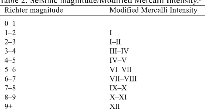
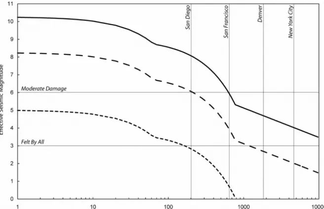
Abstract–We have developed a Web-based program for quickly estimating the regional environmental consequences of a comet or asteroid impact on Earth (www.lpl.arizona.edu/ impacteffects). This paper details the observations, assumptions and equations upon which the program is based. It describes our approach to quantifying the principal impact processes that might affect the people, buildings, and landscape in the vicinity of an impact event and discusses the uncertainty in our predictions. The program requires six inputs: impactor diameter, impactor density, impact velocity before atmospheric entry, impact angle, the distance from the impact at which the environmental effects are to be calculated, and the target type (sedimentary rock, crystalline rock, or a water layer above rock). The program includes novel algorithms for estimating the fate of the impactor during atmospheric traverse, the thermal radiation emitted by the impact-generated vapor plume (fireball), and the intensity of seismic shaking. The program also approximates various dimensions of the impact crater and ejecta deposit, as well as estimating the severity of the air blast in both crater-forming and airburst impacts. We illustrate the utility of our program by examining the predicted environmental consequences across the United States of hypothetical impact scenarios occurring in Los Angeles. We find that the most wide-reaching environmental consequence is seismic shaking: both ejecta deposit thickness and air-blast pressure decay much more rapidly with distance than with seismic ground motion. Close to the impact site the most devastating effect is from thermal radiation; however, the curvature of the Earth implies that distant localities are shielded from direct thermal radiation because the fireball is below the horizon.
INTRODUCTION
Asteroid and comet impacts have played a major role in the geological and biological history of the Earth. It is widely accepted that one such event, 65 million years ago, perturbed the global environment so catastrophically that a major biological extinction ensued (Alvarez 1980). As a result, both the scientific community and the general populace are increasingly interested in both the threat to civilization and the potential environmental consequences of impacts. Previous papers have examined, in detail, the natural hazard associated with the major environmental perturbations caused by impact events (Toon et al. 1994, 1997). To provide a quick and straightforward method for estimating the severity of several of these environmental effects, we have developed a free-of-charge, easy-to-use Web page maintained by the University of Arizona, which is
located at: www.lpl.arizona.edu/impacteffects. Our program focuses on the consequences of an impact event for the regional environment; that is, from the impact location to a few thousand km away. The purpose of this paper is to present and justify the algorithm behind our program so that it may be applied more specifically to important terrestrial impact events and its reliability and limitations may be understood.
Before describing our program in detail, we will briefly review the impact process and the related environmental consequences. The impact of an extraterrestrial object on Earth begins when the impactor enters the tenuous upper atmosphere. At this moment, the impactor is traveling at a speed of between 11 and 72 km s 1 on a trajectory anywhere
between normal incidence (90° to the Earth’s surface) and a grazing impact, parallel to the Earth’s surface. The most likely impact angle is 45° (Shoemaker 1962). The impactor’s
traverse of the atmosphere may disrupt and decelerate the impactor significantly—a process that greatly affects the environmental consequences of the collision. Small impactors are disrupted entirely during their atmospheric traverse, depositing their kinetic energy well above the surface and forming no crater. Larger objects, however, retain sufficient momentum through the atmosphere to strike the Earth with enough energy to excavate a large crater and initiate several processes that affect the local, regional, and even global environment.
The formation of an impact crater is an extremely complicated and dynamic process (Melosh 1989). The abrupt deceleration of a comet or asteroid as it collides with the Earth transfers an immense amount of kinetic energy from the impacting body to the target. As a result, the target and impactor are rapidly compressed to very high pressures and heated to enormous temperatures. Between the compressed and uncompressed material, a shock wave is created that propagates away from the point of impact. In the wake of the expanding shock wave, the target is comprehensively fractured, shock-heated, shaken, and set in motion—leading to the excavation of a cavity many times larger than the impactor itself. This temporary cavity (often termed the transient crater; Dence et al. 1977) subsequently collapses under the influence of gravity to produce the final crater form. As the crater grows and collapses, large volumes of rock debris are ejected onto the surface of the Earth surrounding the crater. Close to the crater rim, this “ejecta deposit” forms a continuous blanket smothering the underlying terrain; further out, the ejecta lands as a scattered assortment of fine-grained dust and larger bombs that may themselves form small secondary craters.
In addition to cratering the surface of the earth, an impact event initiates several other processes that may have severe environmental consequences. During an impact, the kinetic energy of the impactor is ultimately converted into thermal energy (in the impactor and target), seismic energy, and kinetic energy of the target and atmosphere. The increase in thermal energy melts and vaporizes the entire impactor and some of the target rocks. The hot plume of impact-generated vapor that expands away from the impact site (referred to as the “fireball”) radiates thermal energy that may ignite fires and scorch wildlife within sight of the fireball. As the impact-generated shock wave propagates through the target, it eventually decays into elastic waves that travel great distances and cause violent ground shaking several crater radii away. In addition, the atmosphere is disturbed in a similar manner to the target rocks; a shock wave propagates away from the impact site compressing the air to high pressures that can pulverize animals and demolish buildings, vehicles, and infrastructure, particularly where constructional quality is poor. Immediately behind the high-pressure front, violent winds ensue that may flatten forests and scatter debris.
All of these impact-related processes combine and interact in an extremely complicated way that requires detailed observation, laboratory experiments, or computer models to fully simulate and understand. However, with certain simplifying assumptions, we can derive reasonable estimates of their consequences for the terrestrial environment. In the following sections, we describe each of the steps that allow us to achieve this in the Earth Impact Effects Program. We discuss how our program estimates: 1) the impact energy and average time interval between impacts of the same energy, somewhere on Earth; 2) the consequences of atmospheric entry; 3) for crater forming events, the resulting crater size and volume of the melt produced; 4) the thermal radiation damage from the fireball; 5) the impact-induced seismic shaking; 6) the extent and nature of the ejecta deposit; and 7) the damage caused by the blast wave. To clearly identify our algorithm in the following discussion, all of the equations that we implement in the code are labeled with an asterisk (*).
To make the program accessible to the broadest range of users, it was written with as few input parameters as possible. The program requests six descriptors, which are illustrated schematically in Fig. 1: the diameter of the impactor L0 (we use the term impactor to denote the asteroid, comet or other extraterrestrial object considered), the impactor density i, the impact velocity v0, the angle that the trajectory of the impactor subtends with the surface of the Earth at the impact point , the target type, and the distance away from the impact at which the user wishes to calculate the environmental consequences r. Three target types are possible: sedimentary rock, for which we assign a target density of t 2500 kg m3, crystalline rock ( t 2750 kg m 3), or a marine target, for which the program
requests a water-layer depth dw and assigns a density of w 1000 kg m 3 for the water and a target density of
t 2700 kg m 3 for the rock layer below. The program offers the user a
variety of options for units; however, in this paper, the units for all variables are the SI units (mks) unless otherwise stated.
IMPACT ENERGY AND RECURRENCE INTERVAL The most fundamental quantity in assessing the environmental consequences of the impact is the energy released during the impact, which is related to the kinetic energy of the impactor E before atmospheric entry begins. At normal solar system impact speeds, E is approximately given as one half times the impactor mass mi times the square of the impactor velocity v0, which can be rewritten in terms of the meteoroid’s density i and diameter L0, assuming that the meteoroid is approximately spherical:
(1*) In fact, the program uses the relativistic energy equation to accommodate the requests of several science fiction writers. The program does not limit the impact velocity to
E 1 2 ---miv02 12 --- iL03v02 = =
72 km s 1, the maximum possible for an impactor bound to
the Sun; however, we have limited the maximum velocity to the speed of light, in response to attempts of a few users to insert supra-light velocities!
Natural objects that encounter the Earth are either asteroids or comets. Asteroids are made of rock ( i ~2000– 3000 kg m3; Hilton 2002) or iron (
i ~8000 kg m3) and typically collide with the Earth’s atmosphere at velocities of 12–20 km s 1 (Bottke et al. 1994). Detailed knowledge of the
composition of comets is currently lacking; however, they are of much lower density ( i ~500–1500 kg m3) and are composed
mainly of ice (Chapman and Brandt 2004). Typical velocities at which comets might encounter the Earth’s atmosphere are in the range of 30–70 km s 1 (Marsden and Steel 1994). Thus, an
asteroid or comet typically has 4–20 times the energy per unit mass of TNT at the moment atmospheric entry begins. Therefore, impact events have much in common with chemical and nuclear explosions, a fact that we will rely on later in our estimates of the environmental effects of an impact.
Observations of near-Earth objects made by several telescopic search programs show that the number of near-Earth asteroids with a diameter greater than Lkm (in km) may be expressed approximately by the power law (Near-Earth Object Science Definition Team 2003):
N(>L) 1148Lkm 2.354 (2)
These data may also be represented in terms of the recurrence interval TRE in years versus the impact energy EMt in megatons of TNT by assuming a probability of a single-object collision with Earth (~1.6 × 10 9 yr 1; Near-Earth Object
Science Definition Team 2003; their Fig. 2.3) and multiplying by the number of asteroids of a given potential impact energy that are estimated to be circling the sun with potentially hazardous, Earth-crossing orbits. We found that a simple power-law relationship adequately represents these data:
TRE 109EMt0.78 (3*)
Thus, for a given set of user-input impact parameters (L0,
v0, i, t, and ), the program computes the kinetic energy (EMt, in megatons; 1 Mt = 4.18 × 10¹⁵ J) possessed by the
impacting body when it hits the upper atmosphere and defines an average time interval between impacts of that energy, somewhere on the Earth. Furthermore, we estimate the recurrence interval TRL for impacts of this same energy within a certain specified distance r of the impact. This is simply the product of the recurrence interval for the whole Earth and the fraction of the Earth’s surface area that is within the distance r: (4*) where is the epicentral angle from the impact point to a range r (given in radians by: = r/RE, where RE is the radius of the Earth; Fig. 1).
Currently, the relative importance of comets to the Earth-crossing impactor flux is not well-constrained. The Near-Earth Object Science Definition Team (2003) suggests that comets comprise only about 1% of the estimated population of small NEOs; however, there is evidence to suggest that, at larger sizes, comets may comprise a significantly larger proportion of the impactor flux (Shoemaker et al. 1990). Of the asteroids that collide with the Earth’s atmosphere, the current best estimate is that approximately 2–10% are iron asteroids (Bland and Artemieva 2003), based on NEO and main-belt asteroid spectroscopy (Bus et al. 2002; Binzel et al. 2003), meteorite composition, and the impactor types in large terrestrial craters.
ATMOSPHERIC ENTRY
Atmospheric entry of asteroids has been discussed in detail by many authors (Chyba et al. 1993; Ivanov et al. 1997; Krinov 1966; Melosh 1981; Passey and Melosh 1980; Svetsov et al. 1995; Korycansky et al. 2000, 2002; Korycansky and Zahnle 2003, 2004; Bland and Artemieva 2003) and is now understood to be a complex process, involving interaction of the atmosphere and fragmenting impactor in the Earth’s gravitational field. For the purposes of a simple program of the type that we have created, many of the refinements now understood are too complex to be included. Therefore, we have opted to make a number of drastic simplifications that, we believe, will still give a good description of the basic events during atmospheric entry for most cases. Of course, for refined predictions, a full simulation using all of the known processes and properties must be undertaken. Atmospheric entry has no significant influence on the shape, energy, or
Fig. 1. Diagram illustrating the input parameters for the Earth Impact Effects Program: L0 is the impactor diameter at the top of the atmosphere, v0 is the velocity of the impactor at the top of the atmosphere, i is the impactor density, t is the target density, and is the angle subtended between the impactor’s trajectory and the tangent plane to the surface of the Earth at the impact point. The distance r from the impact site at which the environmental consequences are determined is measured along the surface of the Earth; the epicentral angle between the impact point and this distance r is given by = r/RE, where RE is the radius of the Earth.
TRL TRE
2
--- 1 cos– =
momentum of impactors with a mass that is much larger than the mass of the atmosphere displaced during penetration. For this reason, the program procedure described below is applied only for impactors less than 1 km in diameter.
For the purposes of the Earth Impact Effects Program, we assume that the trajectory of the impactor is a straight line from the top of the atmosphere to the surface, sloping at a constant angle to the horizon given by the user. Acceleration of the impactor by the Earth’s gravity is ignored, as is deviation of the trajectory toward the vertical in the case that terminal velocity is reached, as it may be for small impactors. The curvature of the Earth is also ignored. The atmosphere is assumed to be purely exponential, with the density given by:
(z) 0e z/H (5)
where z is the altitude above the surface, H is the scale height, taken to be 8 km on the average Earth, and 0 is the surface atmospheric density, taken to be equal to 1 kg/m3.
During the first portion of the impactor’s flight, its speed is decreased by atmospheric drag, but the stresses are too small to cause fragmentation. Small meteoroids are often ablated to nothing during this phase, but in the current program implementation, we ignore ablation on the grounds that it seldom affects the larger impactors that reach the surface to cause craters. Thus, this program should not be used to estimate the entry process of small objects that may cause visible meteors or even drop small meteorites to the surface at terminal velocity.
While the body remains intact, the diameter of the incoming impactor is constant, equal to the diameter L0 given by the user. The rate of change of the velocity v is given by the usual drag equation (corrected from Melosh 1989, chapter 11): (6) where CD is the drag coefficient, taken to equal 2, and i is the impactor density (an input parameter). This equation can be greatly simplified by making the replacement dt = dz/v sin (justified by our assumption that the impactor travels in a straight line) and rearranging:
(7) Integration of this equation using the exponential density dependence gives the velocity of the impactor as a function of altitude:
(8*) where is the entry angle, and v0 is the impact velocity at the top of the atmosphere, given by the user.
As the impactor penetrates the atmosphere the atmospheric density increases and the stagnation pressure at
the leading edge of the impactor, Ps (z) v(z)2, rises. Eventually, this exceeds the strength of the impactor, and it begins to break up. Observed meteoroids often undergo several cascades of breakup, reflecting components of widely varying strengths. The entire subject of meteoroid strength is poorly understood, as measured crushing strengths of specimens collected on the ground are often a factor of 10 less than strengths inferred from observed breakup (Svetsov et al. 1995). Clearly, strong selection effects are at work. For the purposes of our program, we decided not to embroil the user in the ill-defined guesswork of estimating meteoroid crushing strength. Instead, we found a rough correlation between density and estimated strength for comets (about 15 Pa in tension from the tidal breakup of SL-9; Scotti and Melosh 1993), chondrites (Chyba et al. 1993), and iron or stone objects (Petrovic 2001). Based on four simplified estimates for comets, carbonaceous, stony, and iron meteorites, we established an empirical strength-density relation for use in the program. The yield strength Yi of the impactor in Pa is thus computed from:
(9*) where the impactor density i is in kg m 3. Note that, even at
zero density, this implies a non-zero strength of about 130 Pa. Thus, this empirical formula should not be applied too far out of the range of 1000 to 8000 kg m 3, over which it was
established.
Using this estimate of strength and comparing it to the stagnation pressure, we can compute an altitude of breakup z*
by solving the transcendental equation: Yi = (z*)v2(z
*) (10)
Rather than solving this equation in the program directly, an excellent analytic approximation to the solution was found and implemented:
(11*)
where If is given by:
(12*) In certain specific instances (i.e., small, strong impactors), the impactor may reach the surface intact; in this case, If >1, and Equation 11 does not apply. The properly decremented velocity, calculated using Equation 8, is used to compute a crater size. (If this velocity happens to be less than the terminal velocity, then the maximum of the two is used instead.) The velocity at the top of the atmosphere and at the surface is reported.
Most often, the impactor begins to break up well above the surface; in this case, If <1, and Equation 11 is used to
dv dt --- 3 zCD 4 iL0 ---– v2 = d ln v dz --- 3 z CD 4 iL0sin ---= v z v0 3 z CDH 4 iL0sin ---– exp = log10Yi = 2.107 0.0624+ i z* –H Yi 0vi2 ---ln +1.308 0.314I– f–1.303 1 I– f If 4.07 CDHYi iL0vi2sin ---=
compute the breakup altitude z*. After breakup, the fragments begin to disperse in a complex series of processes (Passey and Melosh 1980; Svetsov et al. 1995) that require detailed numerical treatment. However, a simple approximation to this cascade was found (Chyba et al. 1993; Melosh 1981), called the pancake model, that does a good job for Tunguska-class events. The basic idea of this model is that the impactor, once fractured, expands laterally under the differential pressure between the front and back surfaces. The front of the impactor is compressed at the stagnation pressure, and the rear is essentially in a vacuum with zero pressure. The sides squirt out at a rate determined by force balance in an inviscid fluid. This leads to a simple equation for the expansion of the impactor diameter L, now a function of time:
(13) The initial condition is that L = L0 at z = z*. If L does not increase too much over the scale height H, the time derivatives can be replaced with altitude derivatives (Chyba et al. 1993) and a nonlinear differential equation can be constructed that does not contain v(z):
(14) Again, we construct an analytic approximation to the full solution of this equation, which is adequate for the purposes of the program:
(15*)
where the dispersion length scale l is given by:
(16*) The velocity as a function of altitude is then given by inserting this expression for L(z) into the drag equation and integrating downward from the breakup altitude z*. Because of the rapid expansion of the pancake, the drag rises rapidly as well, and the velocity drops as a double exponential:
(17*)
The crushed impactor spreads laterally until the ratio
L(z)/L0 reaches a prescribed limit, which we call the “pancake factor” fp. In reality, this should be no larger than 2 to 4 (Ivanov et al. 1997), after which the fragments are sufficiently separated that they follow independent flight paths and may
suffer one, or more, further pancake fragmentation events. However, Chyba et al (1993) obtained good agreement with Tunguska-class events using pancake factors as large as 5–10. In this work, we experimented with different factors and settled on a value of 7 to terminate the dispersion of the impactor. The altitude at which this dispersion is obtained is called the “airburst altitude” (zb; see Fig. 2a); it is given by substituting fp = L(z)/L0 into Equation 15 and rearranging:
(18*)
If the airburst occurs above the surface (Fig. 2a), most of the energy is dissipated in the air. We report the airburst altitude zb and the residual velocity of the swarm, which is computed using Equation 17. In this case, the integral in the exponent, evaluated from the airburst altitude to the disruption altitude, is given by:
(19*)
with the definition . The surface impact velocity of the remnants from the airburst vi is also reported as the maximum of the terminal velocity of a fragment half the diameter of the original impactor or the velocity of the swarm as a whole. The spreading velocity at airburst multiplied by the time to impact is added to the breadth of the swarm to estimate the dispersion of what will be a strewn field on the surface. The principal environmental consequence of such an event is a strong blast wave in the atmosphere (see below).
On the other hand, if the pancake does not spread to the limiting size before it reaches the ground (zb 0 in Equation 19; Fig. 2b), the swarm velocity at the moment of impact is computed using Equation 17. In this case, the integral in the exponent, evaluated from the surface (z = 0) to the disruption altitude, is given by:
(20)
The dispersion of the swarm at impact is compared to the estimated transient crater size (see below) and, if it is comparable or larger, then the formation of a crater field is reported, similar to that actually observed at Henbury, Australia. Otherwise, we assume the impact to be a
crater-d2L dt2 --- CDPs iL --- CD z v 2 z iL ---= = Ld2L dz2 --- CD z isin2 ---= L z L0 1 2H l --- 2 z*–z 2H ---exp –1 2 + = l L0 i CD z* ---sin = v z v z* 3 4 ---– CD z* iL03sin --- ez*–z H z z* L2 z dz exp = zb z* 2H 1 l 2H --- fp2–1 + ln – = ez*–z H zburst z* L2 z dz lL02 24 --- 8 3+ 2 3 l H ---- 2+ 2 + = fp2–1 ez*–z H 0 z* L2 z dz H 3L 0 2 3l2 --- 34 l H ---- 2 + ez* H 6e2z* H 16e3z* 2H 3 – – + l H ---- 2–2 =
forming event and use the velocity at the surface to compute a crater size. In either case, the environmental consequences of these events are calculated based on an impact energy equal to the total kinetic energy of the swarm at the moment it strikes the surface.
Although simple, we have found the prescription above to give a fairly reasonable account of atmospheric entry over a wide range of impactor sizes and compositions. As mentioned above, a much more complex treatment must be made on a case-by-case basis if more exact results are needed. In particular, our program is not capable of providing a mass-or velocity-distribution fmass-or fragmented impactmass-ors and, therefore, cannot be used to model production of terrestrial crater fields where the size of the largest crater is related to the largest surviving fragment.
CRATER DIMENSIONS AND MELT PRODUCTION Determining the size of the final crater from a given impactor size, density, velocity, and angle of incidence is not
a trivial task. The central difficulty in deriving an accurate estimate of the final crater diameter is that no observational or experimental data exist for impact craters larger than a few tens of meters in diameter. Perhaps the best approach is to use sophisticated numerical models capable of simulating the propagation of shock waves, the excavation of the transient crater, and its subsequent collapse; however, this method is beyond the scope of our simple program. Instead, we use a set of scaling laws that extrapolate the results of small-scale experimental data to scales of interest or extend observations of cratering on other planets to the Earth. The first scaling law we apply is based on the work of Holsapple and Schmidt (1982), Schmidt and Housen (1987), and Gault (1974) and combines a wide range of experimental cratering data (for example, small-scale hypervelocity experiments and nuclear explosion experiments). The equation relates the density of the target t and impactor i (in kg m 3), the impactor
diameter after atmospheric entry L (in m), the impact velocity at the surface vi (in m s 1), the angle of impact (measured to
the horizontal), and the Earth’s surface gravity gE (in m s 2),
Fig. 2. Schematic illustration of two atmospheric entry scenarios considered in the Earth Impact Effects Program: a) the impactor (initial diameter L0) begins to break up at an altitude z*; from this point the impactor spreads perpendicular to the trajectory due to the different pressures on the front and back face. We define the airburst altitude zb to be the height above the surface at which the impactor diameter L(z) = 7L0. All the impact energy is assumed to be deposited at this altitude; no crater is formed, but the effects of the blast wave are estimated; b) the impactor breaks up but the critical impactor diameter is not reached before the fragmented impactor strikes the surface (z* >0; zb <0). The cluster of fragments impacts the target surface with a velocity vi, forming a single crater or crater field depending on the lateral spread of the cluster, L(z = 0)/sin .
to the diameter of the transient crater Dtc (in m) as measured at the pre-impact target surface (Fig. 3a):
(21*) This equation applies for impacts into solid rock targets where gravity is the predominant arresting influence in crater growth, which is the case for all terrestrial impacts larger than a couple of hundred meters in diameter. For impacts into water, the constant 1.161 must be replaced by 1.365 (Schmidt and Housen 1987). In reality, these constants are not known to three decimal places; the values quoted serve as a best estimate within a range of 0.8 to 1.5.
The transient crater is only an intermediate step in the development of the final crater (Fig. 3). To estimate the final crater diameter, we must consider the effect of the transient
crater’s collapse using another scaling law. For craters smaller than ~3.2 km in diameter on Earth (classified by Dence [1965] as “simple” based on their intuitive morphology), the collapse process is well-understood: highly brecciated and molten rocks that were originally pushed out of the opening crater slide back down the steep transient cavity walls forming a melt-and-breccia lens at the base of the crater (Grieve et al. 1977; Fig. 3a). To derive an estimate of the final crater diameter for simple craters, we applied an analytical model for the collapse of simple craters originally developed by Grieve and Garvin (1984) to two terrestrial craters for which good observational data on breccia-lens volume and final crater dimensions exist. In matching the observational data to model predictions we found that an excellent first order approximation is that the final rim-to-rim diameter Dfr for a simple crater is given approximately by:
Fig. 3. Symbols used in the text to denote the various dimensions of an impact crater. a) Transient crater dimensions: Dtc is the transient crater diameter measured at the pre-impact surface; Dtr is the diameter of the transient crater measured from rim crest to rim crest; htr is the rim height of the transient crater measured from the pre-impact surface; dtc is the depth of the transient crater measured from the pre-impact surface (we assume that Dtc = 2 dtc); b) simple crater dimensions (the transient crater outline is shown by the dotted line): Dfr is the rim-to-rim diameter;
hfr is the rim height above the pre-impact surface; tbr is the breccia lens thickness; dfr is the crater depth measured from the crater floor (above the breccia lens) to the rim crest. We assume that the base of the breccia lens coincides with the floor of the transient crater at a depth of dtc below the pre-impact surface; therefore, dfr = dtc + hfr tbr; c) complex crater dimensions: Dfr is the rim-to-rim diameter; hfr is the rim height above the pre-impact surface; tm is the melt sheet thickness; dfr is the crater depth measured from the crater floor (above the melt sheet) to the rim crest. 2 Dtc 1.161 i t ---- 1 3L0.78vi0.44gE–0.22sin1 3 =
Dfr 1.25Dtc (22*)
if the unbulked breccia lens volume Vbr (i.e., the observed volume of the breccia lens multiplied by a 90–95% bulking correction factor; Grieve and Garvin 1984) is assumed to be related to the final crater diameter by:
Vbr 0.032Dfr3 (23*)
This approximate relationship is based on estimates of unbulked breccia-lens volumes at Meteor Crater and Brent Crater (Grieve and Garvin 1984).
The model may also be used to estimate the thickness of the breccia lens, the depth to the base of the breccia lens, and the final depth of the crater. Assuming that the top surface of the breccia lens is parabolic and that the brecciation process increases the bulk volume of this material by 10%, the thickness of the breccia lens tbr is given approximately by:
(24*) where dtc is the transient crater depth (below the original ground plane), and hfr is the rim height (above the original ground plane) of the final crater (see the section below on ejecta deposits). The depth to the base of the breccia lens is taken to be the same as the transient crater depth dtc, which we assume is given by:
(25*) based on observations by Dence et al. (1977). The depth of the final crater from the rim to the crater floor dfr is then simply (see Fig. 3b):
dfr dtc hfr tbr (26*) For craters larger than 3.2 km on Earth (termed complex because of their unintuitive morphology after Dence [1965]), the collapse process is less well-understood and involves the complicated competition between gravitational forces tending to close the transient crater and the strength properties of the post-impact target rocks. Several scaling laws exist for estimating the rim-to-rim diameter of a complex crater from the transient crater diameter, or vice versa, based on reconstruction of the transient craters of lunar complex craters (see, for example, Croft 1985; McKinnon and Schenk 1985; Holsapple 1993). We use the functional form:
(27*)
established by McKinnon and Schenk (1985), which lies intermediate between the estimates of Croft (1985) and
Holsapple (1993). In this equation, Dc is the diameter at which the transition from simple to complex crater occurs (taken to be 3.2 km on Earth); both Dtc and Dfr are in km (See Fig. 3b). If the transient crater diameter is greater than 2.56 km, we apply Equation 27 to determine the final crater diameter and report that a “complex” crater is formed; otherwise, we apply Equation 22 and report that a “simple” crater is formed. It is worth emphasizing that the final crater diameter that the program reports is the diameter of the fresh crater measured from rim crest to rim crest (see Figs. 3b and 3c). The topographic rim is likely to be strongly affected by post-impact erosion. Furthermore, multiple concentric zones of structural deformation are often observable at terrestrial impact structures—a fact that has led to uncertainty in the relationship between the structural (apparent) and topographic (rim-to-rim) crater diameter (Turtle et al. 2005). Therefore, the results of the scaling arguments above should be compared with caution to apparent diameters of known terrestrial impact structures.
To estimate the average depth dfr (in km) from the rim to floor of a complex crater of rim-to-rim diameter Dfr (in km), we use the depth-to-diameter relationship of Herrick et al. (1997) for venusian craters:
dfr = 0.4Dfr0.3 (28*)
The similarity in surface gravity between Earth and Venus as well as the large number of fresh complex craters on Venus makes this relationship more reliable than that based on the limited and erosion-affected data for terrestrial complex craters (Pike 1980; Grieve and Therriault 2004).
We also estimate the volume of melt produced during the impact event, based on the results of numerical modeling of the early phase of the impact event (O’Keefe and Ahrens 1982b; Pierazzo et al. 1997; Pierazzo and Melosh 2000) and geological observation at terrestrial craters (Grieve and Cintala 1992). Provided that: 1) the impact velocity is in excess of ~12 km s 1 (the threshold velocity for significant
target melting, O’Keefe and Ahrens 1982b); 2) the density of the impactor and target are comparable; and 3) all impacts are vertical, these data are well-fit by the simple expression:
(29) where Vm is the volume of melt produced, Vi is the volume of the impactor, and m is the specific energy of the Rankine-Hugoniot state from which the isentropic release ends at the 1 bar point on the liquidus. To avoid requiring further input parameters in our program, we use m = 5.2 MJ/kg for granite (see Pierazzo et al. 1997), which we take as representative of upper-crustal rocks, and assume an impactor and target density of 2700 kg m 3. This allows us to rewrite Equation 29,
giving the impact melt volume Vm (in m3) in terms of just the
impact energy E (in J): Vm = 8.9 × 10¹²E.
To account for the effect of impact angle on impact melt
tbr 2.8Vbr dtc+hfr dtcDfr2 ---= dtc = Dtc 2 2 Dfr 1.17Dtc 1.13 Dc0.13 ---= Vm 0.25vi 2 m ---Vi =
production, we assume, based on numerical modeling work (Pierazzo and Melosh 2000; Ivanov and Artemieva 2002), that the volume of impact melt is roughly proportional to the volume of the transient crater. In our program, the diameter and depth of the transient crater are proportional to sin1/3
(Equations 21 and 25); hence, the volume of the transient crater is proportional to sin . The equation used in our program to compute the impact melt volume is, therefore:
Vm = 8.9 × 10 12 E sin (30*)
This expression works well for all geologic materials except ice. In this case, Vm is about ten times larger than for rock (Pierazzo et al. 1997). Equation 30 neglects the effect of geothermal gradient on melt production. For very large impacts, which affect rocks deep in the Earth where ambient temperatures are much closer to the melting point, this expression will underestimate the volume of melt produced. Equation 30 agrees well with model predictions (Pierazzo and Melosh 2000) of impact melt volume versus impact angle for impact angles greater than ~15 to the horizontal; for impact angles of ~15 or less, Equation 30 probably overestimates the volume of impact melt produced by a factor of ~2.
In simple craters, the melt is well-mixed within the breccia lens on the floor of the crater; in larger complex craters, however, the melt forms a coherent sheet, which usually has an approximately uniform thickness across the crater floor (Grieve et al. 1977). Here we assume that the crater floor diameter is similar to the transient crater diameter (Croft 1985). Thus, we estimate the average thickness of this sheet tm as the ratio of the melt volume to the area of a circle equal in diameter to the transient crater:
tm = 4Vm/ Dtc2 (31*)
In extremely large terrestrial impact events (Dtc
>1500 km), the volume of melt produced, as predicted by Equation 30, is larger than the volume of the crater. In this case, we anticipate that the transient crater would collapse to a hydrostatic, almost-featureless surface and, therefore, our program does not quote a final crater diameter. Instead of a topographically observable crater, the program postulates that a large circular melt province would be formed. We note, however, that no such feature has been unequivocally identified on Earth. Our program also compares the volume of impact-generated melt to the volume of the Earth and reports the fraction of the planet that is melted in truly gigantic impacts.
THERMAL RADIATION
As alluded to above, the compression of the target and impactor during the initial stages of an impact event drastically raises the temperature and pressure of a small region proximal to the impact site. For impacts at a velocity greater than ~12 km s 1, the shock pressures are high enough
to melt the entire impactor and some target material;
vaporization also occurs for impacts at velocities greater than ~15 km s 1. Any vapor produced is initially at very high
pressure (>100 GPa) and temperature (>10,000 K) and, thus, begins to rapidly inflate; the expanding hot vapor plume is termed the “fireball.” The high temperatures imply that thermal radiation is an important part of the energy balance of the expanding plume. Initially, the fireball is so hot that the air is ionized and its radiation absorption properties are substantially increased. As a result, the fireball is initially opaque to the emitted radiation, which remains bottled up within the ball of plasma. The actual process is much more complex than the simple description here and we refer the interested reader to Glasstone and Dolan (1977) for a more complete exposition. With continued expansion, the fireball cools; as the temperature approaches a critical temperature, known as the transparency temperature T* (Zel’dovich and Raizer 1966, p. 607), the opacity rapidly diminishes and the thermal radiation escapes, bathing the Earth’s surface in heat from the fireball. The thermal radiation lasts for a few seconds to a few minutes; the radiation intensity decays as the expanding fireball rapidly cools to the point where radiation ceases. For Earth’s atmosphere, the transparency temperature is ~2000–3000 K (Nemtchinov et al. 1998); hence, the thermal radiation is primarily in the visible and infrared wavelengths—the fireball appears as a “second sun” in the sky. The transparency temperature of silicate vapor is about 6000 K (Melosh et al. 1993), so that the limiting factor for terrestrial impacts is the transparency temperature of air surrounding the silicate vapor fireball.
Provided that the impact velocity is in excess of 15 km s 1,
we estimate the fireball radius Rf* at the moment the transparency temperature is achieved, which we consider to be the time of maximum radiation. Numerical simulations of vapor plume expansion (Melosh et al. 1993; Nemtchinov et al. 1998) predict that the fireball radius at the time of maximum radiation is 10–15 times the impactor diameter. We use a value of 13 and assume “yield scaling” applies to derive a relationship between impact energy E in joules and the fireball radius in meters:
Rf* 0.002E1/3 (32*)
Yield scaling is the empirically derived concept that certain length and time scales measured for two different explosions (or impacts) are approximately identical if divided by the cube root of the yield (or impact) energy. Yield scaling can be justified theoretically, provided that gravity and rate-dependent processes do not strongly influence the measured parameters (Melosh 1989, p. 115). The constant in Equation 32 was found by dividing the fireball radius (given by Rf* 13L0) by the cube root of the impact energy (given by
Equation 1), for a typical impactor density (2700 kg m 3) and
terrestrial impact velocity (20 km s 1).
The time at which thermal radiation is at a maximum Tt is estimated by assuming that the initial expansion of the fireball occurs at approximately the same velocity as the impact:
(33*) To calculate the environmental effects of the thermal radiation from the fireball, we consider the heating at a location a distance r from the impact site. The total amount of thermal energy emitted as thermal radiation is some small fraction (known as the “luminous efficiency”) of the impact energy E. The luminous efficiency for hypervelocity impacts is not presently well-constrained. Numerical modeling results (Nemtchinov et al. 1998) suggest that scales as some power law of impact velocity. The limited experimental, observational, and numerical results that exist indicate that for typical asteroidal impacts with Earth, is in the range of 10 4–10 2 (Ortiz et al. 2000); for a first-order estimate we
assume = 3 × 10 3 and ignore the poorly-constrained
velocity dependence.
The thermal exposure quantifies the amount of heating per unit area at our specified location. is given by the total amount of thermal energy radiated E divided by the area over which this energy is spread (the surface area of a hemisphere of radius r, 2 r2):
(34*) The total thermal energy per unit area that heats our location of interest arrives over a finite time period between the moment the fireball surface cools to the transparency temperature and is unveiled to the moment when the fireball has expanded and cooled to the point where radiation ceases. We define this time period as the “duration of irradiation” t. Without computing the hydrodynamic expansion of the vapor plume this duration may be estimated simply by dividing the total energy radiated per unit area (total thermal energy emitted per unit area of the fireball) by the radiant energy flux, given by T*4, where = 5.67 × 10 8 W m 2 K 4 is the
Stefan-Bolzmann constant. In our program, we use T* = 3000 K. Then, the duration of irradiation is:
(35*)
For situations where the specified distance away from the impact point is so far that the curvature of the Earth implies that part of the fireball is below the horizon, we modify the thermal exposure by multiplying by the ratio f of the area of the fireball above the horizon to the total area. This is given by:
(36*) In this equation, h is the maximum height of the fireball below the horizon as viewed from the point of interest, given by:
h (1 cos )RE (37*)
where is the epicentral angle between the impact point and the point of interest, and RE is the radius of the Earth. If
h Rf*, then the fireball is entirely below the horizon; in this case, no direct thermal radiation will reach our specified location. The angle in Equation 36 is half the angle of the segment of the fireball visible above the horizon, given by
cos 1 h/R
f*. We presently ignore atmospheric refraction and extinction for rays close to the horizon (this effect is important only over a small range interval).
Whether a particular material catches fire as a result of the fireball heating depends not only on the corrected thermal exposure f but also on the duration of irradiation. The thermal exposure ignition (J m 2) required to ignite a material, that is, to heat the surface to a particular ignition temperature
Tignition, is given approximately by:
(38) where is the density, cp is the heat capacity, and is the thermal diffusivity of the material being heated. This expression equates the total radiant energy received per unit area, on the left, to the heat contained in a slab of unit area perpendicular to the fireball direction, on the right. The thickness of the slab is estimated from the depth, , penetrated by the thermal wave during the irradiation time t. Analysis of Equation 35 shows that t is proportional to the thermal exposure divided by the fireball radius squared. Hence, the duration of irradiation is proportional to E1/3, and
the thermal exposure required to ignite a given material is proportional to E1/6. This simple relationship is supported by
empirical data for the ignition of various materials by thermal radiation from nuclear explosion experiments over a range of three orders of magnitude in explosive yield energy (Glasstone and Dolan 1977, p. 287–289). Thus, although a more energetic impact event, or explosion, implies a greater total amount of thermal radiation, this heat arrives over a longer period of time, and hence, there is more time for heat to be diluted by conduction through the material. This results in a greater thermal exposure being required to ignite the same material during a more energetic impact event.
To account for the impact-energy dependence of the thermal exposure required to ignite a material (or cause skin damage), we use a simple scaling law. We estimate the thermal exposure required to ignite several different materials, or burn skin, during an impact of a given energy by multiplying the thermal exposure required to ignite the material during a 1 Mt event (see Table 1; data from Glasstone and Dolan 1977, p. 287–289) by the impact energy (in MT) to the one-sixth power:
ignition(E) ignition(1 Mt)EMt1/6 (39*)
To assess the extent of thermal radiation damage at our location of interest, we compute the thermal radiation
Tt Rf* vi ---= E 2 r2 ---= t E 2 Rf*2 T*4 ---= f 2--- h Rf* --- sin – = ignition Tignition cp t t
exposure f and compare this with ignition (calculated using Equation 39) for each type of damage in Table 1. For thermal exposures in excess of these ignition exposures, we report that the material ignites or burns.
Our simple thermal radiation model neglects the effect of both atmospheric conditions (cloud, fog, etc.) and the variation in atmospheric absorption with altitude above the horizon. Experience from nuclear weapons testing (Glasstone and Dolan 1977, p. 279) suggests that, in low visibility conditions, the reduction in direct (transmitted) radiation is compensated for, in large part, by indirect scattered radiation for distances less than about half the visibility range. This observation led Glasstone and Dolan (1977) to conclude that “as a rough approximation, the amount of thermal energy received at a given distance from a nuclear explosion may be assumed to be independent of the visibility.” Hence, although the above estimate should be considered an upper estimate on the severity of thermal heating, it is probably quite reliable, particularly within half the range of visibility.
SEISMIC EFFECTS
The shock wave generated by the impact expands and weakens as it propagates through the target. Eventually, all that remains are elastic (seismic) waves that travel through the ground and along the surface in the same way as those excited by earthquakes, although the structure of the seismic waves induced by these distinct sources is likely to be considerably different.
To calculate the seismic magnitude of an impact event, we assume that the “seismic efficiency” (the fraction of the kinetic energy of the impact that ends up as seismic wave energy) is one part in ten thousand (1 × 10 4). This value is the
most commonly accepted figure based on experimental data (Schultz and Gault 1975), with a range between 10 5–10 3.
Using the classic Gutenberg-Richter magnitude energy relation, the seismic magnitude M is then:
M 0.67log10 E 5.87 (40*)
where E is the kinetic energy of the impactor in Joules (Melosh 1989, p. 67).
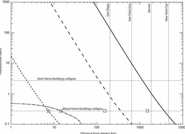
To estimate the extent of devastation at a given distance from a seismic event of this magnitude we determine the intensity of shaking I, as defined by the Modified Mercalli Intensity Scale (see Table 2), the most widely-used intensity scale developed over the last several hundred years to evaluate the effects of earthquakes. We achieve this by defining an “effective seismic magnitude” as the magnitude of an earthquake centered at our specified distance away from the impact that produces the same ground motion amplitude as would be produced by the impact-induced seismic shaking. We then use Table 3, after Richter (1958), to relate the effective seismic magnitude to the Modified Mercalli Intensity. A range of intensities is associated with a given seismic magnitude because the severity of shaking depends on the local geology and rheology of the ground and the propagation of teleseismic waves; for example, damage in alluviated areas will be much more severe than on well-consolidated bed rock.
The equations for effective seismic magnitude use curves fit to empirical data of ground motion as a function of distance from earthquake events in California (Richter 1958, p. 342). We use three functional forms to relate the effective seismic magnitude Meff to the actual seismic magnitude M and the distance from the impact site rkm (in km), depending on the distance away from the impact site. For rkm <60 km:
Meff M 0.0238rkm (41a*) for 60 rkm <700 km:
Meff M 0.0048rkm 1.1644 (41b*) and for rkm 700 km:
Meff M 1.66log10 6.399 (41c*)
To compute the arrival time Ts of the most violent seismic shaking, we assume that the main seismic wave energy is that associated with the surface waves. Then, Ts is simply the user-specified distance rkm (in km) divided by the typical surface-wave velocity of upper-crustal rocks (~5 km s 1):
(42*) Table 1. Ignition factors for various materials.a
Material
Thermal exposure required to ignite material during a 1 Mt explosion ( ignition(1 Mt), MJ m 2) Clothing 1.0 Plywood 0.67 Grass 0.38 Newspaper 0.33 Deciduous trees 0.25
Third degree burns 0.42 Second degree burns 0.25 First degree burns 0.13
aData extracted from Glasstone and Dolan (1977).
Table 2. Seismic magnitude/Modified Mercalli Intensity.a
Richter magnitude Modified Mercalli Intensity
0–1 – 1–2 I 2–3 I–II 3–4 III–IV 4–5 IV–V 5–6 VI–VII 6–7 VII–VIII 7–8 IX–X 8–9 X–XI 9+ XII
aBased on data from Richter (1958).
Ts rkm 5 ---=
EJECTA DEPOSIT
During the excavation of the crater, material originally situated close to the target surface is either thrown out of the crater on ballistic trajectories and subsequently lands to form the ejecta deposit, or is merely displaced upward and outward to form part of the crater rim. This uplifted portion of the crater-rim material is significant close to the transient crater rim but decreases rapidly with distance such that, outside two transient-crater radii from the crater center, the material above the pre-impact target surface is almost all ejecta deposit. For simplicity, we ignore the uplifted fraction of the crater rim material. We estimate the thickness of ejecta at a given distance from an impact by assuming that the material lying above the pre-impact ground surface is entirely ejecta, that it has a maximum thickness te htr at the transient crater rim, and that it falls off as one over the distance from the crater rim cubed:
(43) The power of 3 is a good approximation of data from explosion experiments (McGetchin et al. 1973) and a satisfactory compromise for results from numerical calculations of impacts and shallow-buried nuclear explosions, which show that the power can vary between 2.5 and 3.5.
The ejecta thickness at the transient crater rim (assumed to be equal to the transient crater rim height htr) may be calculated from a simple volume conservation argument where we equate the volume of the ejecta deposit and uplifted
transient crater rim Ve with the volume of the transient crater below the pre-impact surface Vtc. For this simple model, we assume that the transient crater is a paraboloid with a depth to diameter ratio of 1:2 . Ve is given by:
(44)
where Dtr is the diameter of the transient crater at the transient crater rim (see Fig. 3a), which is related to Dtc by:
(45)
The volume of the transient crater is given by:
(46) Equating Ve with Vtc and rearranging to find the rim height gives htr = Dtc/14.1. Inserting this result into Equation 43 gives the simple expression used in the program: (47*) Table 3. Abbreviated version of the Modified Mercalli Intensity scale.
Intensity Description
I Not felt except by a very few under especially favorable conditions. II Felt only by a few persons at rest, especially on upper floors of buildings.
III Felt quite noticeably by persons indoors, especially on upper floors of buildings. Many people do not recognize it as an earthquake. Standing motor cars may rock slightly. Vibrations similar to the passing of a truck.
IV Felt indoors by many, outdoors by few during the day. At night, some awakened. Dishes, windows, doors disturbed; walls make cracking sound. Sensation like heavy truck striking building. Standing motor cars rocked noticeably.
V Felt by nearly everyone; many awakened. Some dishes, windows broken. Unstable objects overturned. Pendulum clocks may stop.
VI Felt by all, many frightened. Some heavy furniture moved; a few instances of fallen plaster. Damage slight.
VII Damage negligible in buildings of good design and construction; slight to moderate in well-built ordinary structures; considerable damage in poorly built or badly designed structures; some chimneys broken.
VIII Damage slight in specially designed structures; considerable damage in ordinary substantial buildings with partial collapse. Damage great in poorly built structures. Fall of chimneys, factory stacks, columns, monuments, and walls. Heavy furniture overturned.
IX General panic. Damage considerable in specially designed structures; well-designed frame structures thrown out of plumb. Damage great in substantial buildings, with partial collapse. Buildings shifted off foundations. Serious damage to reservoirs. Underground pipes broken. Conspicuous cracks in ground. In alluviated areas sand and mud ejected, earthquake fountains, sand craters.
X Most masonry and frame structures destroyed with their foundations. Some well-built wooden structures and bridges destroyed. Serious damage to dams, dikes, and embankments. Large landslides. Water thrown on banks of canals, rivers, lakes, etc. Sand and mud shifted horizontally on beaches and flat land. Rails bent slightly.
XI As X. Rails bent greatly. Underground pipelines completely out of service.
XII As X. Damage nearly total. Large rock masses displaced. Lines of sight and level distorted. Objects thrown into the air.
te htr 8 --- dtr r --- 3 = 2 Ve htrDtr 3 8 --- 2 rdr r3 ---Dtr 2 2 r Dtc 2 Dtr 2 + 4dtc Dtc2 ---r2–dtc dr = 2 --- htrDtr2 dtc Dtr 4 D tc 4 – 4Dtc2 --- Dtr 2 D tc 2 – 2 ---– + = Dtr Dtc dtc+htr dtc ---= Vtc Dtc 3 16 2 ---= te Dtc 4 112r3 ---=
As this model ignores any “bulking” of the ejecta deposit and entrainment of the substrate on which the ejecta lands, it provides a lower bound on the probable ejecta thickness. The use of transient crater diameter instead of final crater diameter avoids the need for a separate rim height equation for simple and complex craters. Rim heights of complex craters, as a fraction of the final crater diameter, are significantly smaller than the scaled rim heights of simple craters because, for complex craters, the thickest part of the ejecta blanket collapses back into the final crater during the late stages of the cratering process. As this collapse process is not fully understood, we only report the ejecta thickness outside the final crater rim. The final rim height of the crater, which is required for our estimate of the breccia-lens thickness in simple craters (above) is found by inserting r = Dfr/2 into Equation 31:
(48*)
The outward flight of rock ejected from the crater occurs in a transient, rarefied atmosphere within the expanding fireball. In large impacts (E >200 Mt), the fireball radius is comparable to the scale height of the atmosphere; hence, the ejecta’s trajectory takes it out of the dense part of the atmosphere, allowing it to reach distances much in excess of the fireball radius. For smaller impacts, however, the ejecta’s outward trajectory is ultimately stifled at the edge of the fireball, where the atmospheric density returns to normal. We incorporate these considerations into our program by limiting the spatial extent of the ejecta deposit to the range of the fireball for impact energies less than 200 Mt.
The ejecta arrival time is determined using ballistic travel time equations derived by Ahrens and O’Keefe (1978) for a spherical planet. Using a mean ejection angle of 45° to the Earth’s surface allows us to estimate the approximate arrival time of the bulk of the ejecta. In reality, material is ejected from the crater at a range of angles, and consequently, the arrival of ejecta at a given location does not occur simultaneously. However, this assumption allows us to write down an exact (although complex) analytical expression for the average travel time of the ejecta Te to our specified location:
(49*)
where RE is the radius of the Earth, gE is the gravitational acceleration at the surface of the Earth, and is the epicentral angle between the impact point and the point of interest. The ellipticity e of the trajectory of ejecta leaving the impact site at an angle of 45° to the horizontal and landing at the point of interest is given by:
(50*) where ve is the ejection velocity, and e is negative when ve2/
gERE 1. The semi-major axis a of the trajectory is given by: (51*) To compute the ejection velocity of material reaching the specified range r RE, we use the relation:
(52*) which assumes that all ejecta is thrown out of the crater from the same point and at the same angle (45°) to the horizontal.
Equation 49 is valid only when ve2/g
ERE 1, which corresponds to distances from the impact site less than about 10,000 km (1/4 of the distance around the Earth). For distances greater than this, a similar equation exists (Ahrens and O’Keefe 1978); however, we do not implement it in our program because, in this case, the arrival time of the ejecta is much longer than one hour. Consequently, an accurate estimate of ejecta thickness at distal locations must take into account the rotation of the Earth, which is beyond the scope of our simple program. Furthermore, ejecta traveling along these trajectories will be predominantly fine material that condensed out of the vapor plume and will be greatly affected by reentry into the atmosphere, which is also not considered in our current model. For ejecta arrival times longer than one hour, therefore, the program reports that “little rocky ejecta reaches our point of interest; fallout is dominated by condensed vapor from the impactor.”
We also estimate the mean fragment size of the fine ejecta at our specified location using results from a study of parabolic ejecta deposits around venusian craters (Schaller and Melosh 1998). These ejecta deposits are thought to form by the combined effect of differential settling of fine ejecta fragments through the atmosphere depending on fragment size (smaller particles take longer to drop through the atmosphere), and the zonal winds on Venus (Vervack and Melosh 1992). Schaller and Melosh (1998) compared a theoretical model for the formation of the parabolic ejecta deposits with radar observations and derived an empirical law for the mean diameter of impact ejecta d (in m) on Venus as a function of distance from the crater center rkm (in km):
(53*) where Dfr is the final crater diameter measured from rim to rim (in km); 2.65, and dc 2400(Dfr/2) 1.62. This relation
neglects the effects of the atmosphere and wind transportation on Earth, which will be more significant for
hfr 0.07Dtc 4 Dfr3 ---= Te 2a 1.5 gERE2 --- 2 –1 1 e– 1 e+ ---4 ---tan e 1 e 2 – sin 2 1 e+ cos 2 ---– tan = e2 1 2 --- ve 2 gERE --- 1– 2 1 + = a ve 2 2gE 1 e– 2 ---= ve2 2gEREtan 2 1+tan 2 ---= d dc Dfr 2rkm ---=
smaller fragment sizes, and the disintegration of ejecta particles as they land. Thus, the uncertainty in these predictions is greatest very close to the crater, where ejecta fragments are large and will break up significantly during deposition, and at great distances from the impact point, where the predicted fragment size is small. We circumvent this problem at small distances by not calculating the mean fragment size for ranges less than two crater radii, which roughly corresponds to the extent of the continuous ejecta blanket observed around extra-terrestrial craters (Melosh 1989, p. 90). We also emphasize that the predicted fragment size is a rough mean value of the ejecta fragment size. At any given location, there will be a range of fragment sizes around this mean including large bombs and very fine-grained dust, which will arrive at different times depending on how easily they traverse the atmosphere.
AIR BLAST
The impact-induced shock wave in the atmosphere is referred to as the air blast or blast wave. The intensity of the blast depends on the energy released during the impact and the height in the atmosphere at which the energy is deposited, which is either zero for impacts where a crater is formed or the burst altitude for airburst events. The effects of the blast wave may be estimated by drawing on data from US nuclear explosion tests (Glasstone and Dolan 1977; Toon et al. 1994, 1997; Kring 1997). The important quantities to determine are the peak overpressure, that is, the maximum pressure in excess of the ambient atmospheric pressure (1 bar = 105 Pa),
and the ensuing maximum wind speed. With these data, tables compiled by the US Department of Defense may be used to predict the damage to buildings and structures of varying constructional quality, vehicles, windows, and trees.
To estimate the peak overpressure for crater-forming impacts, we assume that the impact-generated shock wave in the air is directly analogous to that generated by an explosive charge detonated at the ground surface (surface burst). We found that the expression:
(54*) is an excellent fit to empirical data on the decay of peak overpressure p (in Pa) with distance r1 (in m) for a 1 kiloton (kt) surface burst (Glasstone and Dolan 1977; their Fig. 3.66, p. 109). In this equation, the pressure px at the crossover point from ~1/r2.3 behavior to ~1/r behavior is 75000 Pa
(0.75 bars); this occurs at a distance of 290 m.
The peak overpressure resulting from an airburst is estimated using a similar suite of equations fit to empirical data on the peak overpressure experienced at different distances away from explosions detonated at various heights above the surface (Glasstone and Dolan 1977, p. 113). The relationship between peak overpressure and distance away
from ground zero (the location on the Earth directly below the airburst) is more complex than for a surface burst due to the interaction between the blast wave direct from the source and the wave reflected off the surface. Within a certain distance from ground zero, the delay between the arrival of the direct wave and the reflected wave is sufficient for little constructive interference of the waves to occur; this region is known as the regular reflection region. Beyond this zone, however, the two waves merge in what is known as the “Mach reflection region;” this effect can increase the overpressure at a given location by as much as a factor of two (Glasstone and Dolan 1977, p. 38). Within the Mach region, we found that Equation 54 holds approximately, provided that the crossover distance
rx is increased slightly as a function of burst altitude (rx 289 0.65zb). At distances inside the regular reflection region, we found that the peak overpressure decreases exponentially with distance from ground zero:
(55*) where p0 and are both functions of burst altitude:
p0 3.14 × 10¹¹z
b 2.6 (56a*)
34.87zb 1.73 (56b*)
To extrapolate these relationships to explosions (impacts) of greater energy, we again rely on yield scaling, which implies that a specific peak overpressure occurs at a distance from an explosion that is proportional to the cube root of the yield energy. In other words, the ratio of the distance at which a certain peak overpressure occurs to the cube root of the impact energy (r(p)/E1/3) is constant for all impacts.
Therefore, the peak overpressure at the user-specified distance r away from an impact of energy Ekt (in kilotons) is the same as that at a distance r1 away from an impact of energy 1 kt, where r1 is given by:
(57*) The equivalent burst altitude in a 1 kt explosion zb1 is related to the actual burst altitude by a similar equation zb1 zb/Ekt1/3.
To compute the peak overpressure, we substitute the scaled-distance r1 into Equation 54 or 55, depending on whether the distance r1 lies within the Mach region or the regular reflection region for a 1 kt explosion. The distance from ground zero to the inner edge of the Mach region rm1 in such an explosion depends only on the altitude of burst zb1; we found a good fit to the observational data with the simple function: (58*) p pxrx 4r1 --- 1 3 rx r1 ---- 1.3 + = p p0e– r1 = r1 r EkT1 3 ---= rm1 550zb1 1.2 550 z– b1 ---=