Techniques for augmenting the visualisation of dynamic raster surfaces

CENTRE FOR

ADV

ANCED

SP

A

TIAL

ANAL

YSIS

W

orking Paper Series

Paper 59

TECHNIQUES FOR

AUGMENTING THE

VISUALISATION OF

DYNAMIC RASTER

SURFACES

Centre for Advanced Spatial Analysis University College London

1-19 Torrington Place Gower Street

London WC1E 6BT

[t] +44 (0) 20 7679 1782 [f] +44 (0) 20 7813 2843 [e] [email protected] [w] www.casa.ucl.ac.uk

http//www.casa.ucl.ac.uk/working_papers/paper59.pdf

Date: November 2002

ISSN: 1467-1298

© Copyright CASA, UCL

Techniques for augmenting the visualisation of dynamic raster surfaces

Sanjay Rana and Jason Dykes†

Centre for Advanced Spatial Analysis, University College London, 1-19 Torrington Place, London WC1E 6BT, UK

†

Department of Information Science, City University, London EC1V OHB

Techniques for augmenting the visualisation of dynamic raster surfaces

Sanjay Rana Jason Dykes

Centre for Advanced Spatial Analysis Department of Information Science

University College London City University

London WC1E 6BT London EC1V OHB

[email protected] [email protected]

Abstract

Despite their aesthetic appeal and condensed nature, dynamic raster surface representations

such as a temporal series of a landform and an attribute series of a socio-economic attribute of

an area, are often criticised for the lack of an effective information delivery and interactivity.

In this work, we readdress some of the earlier raised reasons for these limitations -

information-laden quality of surface datasets, lack of spatial and temporal continuity in the

original data, and a limited scope for a real-time interactivity. We demonstrate with examples

that the use of four techniques namely the re-expression of the surfaces as a framework of

morphometric features, spatial generalisation, morphing, graphic lag and brushing can

1. Introduction

Cartographers and researchers in the scientific- and cartographic- visualisation fields have

produced dynamic maps or animated maps over the last three decades, initially as paper-based

cartoons and, after the eighties, in the form of sophisticated 2D and 3D digital representations.

Although it is generally accepted that dynamic maps are a simple and appealing way of

providing a mental model of the dynamic information, their effectiveness has been debated

from as early as the 1960’s (Bertin, 1967). Recent works that have raised doubts on the

effectiveness of dynamic map include Slocum et al. (1990), Ogao and Kraak (2001), Ogao

and Block (2001), and Emmer (2001). Despite the general apprehension, there is a consensus

that the most suitable visual representation of large information collected over continuous

long period, such as weather (Earnshaw and Watson, 1993) and landscape processes (Mitas et

al., 1997), and multiple attributes would be an dynamic map. Other supporters of dynamic

maps including those who have suggested ways to alleviate the limitations of dynamic maps

include Hayward (1984), Koussoulakou (1990), Dibiase et al. (1992), McCloud (1993),

Peterson (1993), and MacEachren (1994).

Bertins’ main criticism of dynamic maps is that the presence of motion distracts a

user’s attention from the important visual variables such as size, colour, and others, thereby

resulting in a limited interpretation. In other words, a dynamic map necessitates an active

attention to interpret the stream of information. In response to this issue, Dibiase et al. (1992)

and MacEachren (1994) proposed the addition of controls called dynamic visual variables,

such as duration, rate of change, frequency, display time and others to manage the flux of

information available during an animation. In essence, the purpose of dynamic visual

variables is to allow a user-defined attention period to interpret the dynamic information.

However, in the absence of formal and generic guidelines on the use of these controls, we

believe that Bertins’ objection is still not satisfied.

Another demanding requirement and limitation has been the interactive visualisation

of the dynamic maps. Refer to Ware (2000) for an overview of the issues related to interacting

with visualisation. Despite the development of excellent two-dimensional (cdv – Dykes,

1999) and three-dimensional (Kreuseler, 2000) visualisation systems, interactivity in dynamic

maps remains a challenge. Recently, Ogao and Kraak (2001) and Ogao and Block (2001)

have objected about the passivity of dynamic map animations and thus raised issues such as

their limited exploratory capabilities.

We believe that the limitations mentioned above arise due to practical and conceptual

bottlenecks. Certainly, our hardware and software to render satisfactory animation with

interactivity in dynamic maps has been improving all the time (Earnshaw and Watson, 1993;

The conceptual limitations are more ill defined and vague but it is something we can address

without requiring a research expertise in hardware limitation. We posed the following two

conceptual questions to us:

(i) Is there an information overload (also raised by Gahegan, 1999), which is causing the

distraction and poor retention?

(ii) Could the lack of a spatial and temporal continuity within our dynamic map series be

the cause of a limited interpretation?

2. Methodology

2.1 Proposal

For simplicity, we decided to address a specific case of dynamic maps in our investigation

viz. The widely used raster surfaces e.g., digital elevation models (DEMs) and population

density surfaces. Formally, a surface in this work refers to a rasterised smooth doubly

continuous function (i.e., no holes or overhangs) of the form

z

=

f

(

x

,

y

)

z

property (e.g., elevation, population density etc.) being mapped and associated with a point

)

,

(

x

y

well.

Dynamic raster surfaces can broadly belong to two types of dynamic map processes

namely the temporal series and the attribute series. A temporal series depicts the

transformation of a property of the surface from a state

z

t

i.e.,

'

'

t

z

z

→

On the other hand, by attribute series generally depicts the different states of a property say

z

t

t t

z

z

→

'

For example, the animation of the evolution of a landscape over a period of time constitutes a

temporal series (Mitas et al., 1997) while the animation of the population density for the

different age groups of a city in a year should be regarded as an attribute series.

We will now introduce a visualisation strategy composed of three techniques for

2.1.1 Ensure high or increased spatial- and temporal- continuity

A coarse spatial- and thematic- resolution of raster surfaces results into a stepped appearance

that makes it difficult to understand and identify spatial patterns in the surfaces (Herzog,

1993). For instance, the population density surfaces in Figure 1 have spatial resolution of 200

m, which in a thematic sense has been found to be the most appropriate resolution for the

description of the distribution (URL#1) but it is clearly not appealing for the visualisation

purpose. While in temporal datasets, sometimes due to practical limitations the sampling of

surface datasets cannot be done frequently enough to create a continuous temporal series. This

leads to abrupt jumps in the visualisation of dynamic surfaces.

Openshaw et al. (1994) suggested the use of density estimation methods such as proposed

by Gatrell (1994) and Bracken (1994) for creating a smooth map display of socio-economic

data. In a recent work, Paddenburg and Wachowicz (2001) studied the use of spatial

generalisation to reduce noise in raster surfaces and concluded that this pre-processing reveals

the true information otherwise suppressed by the noise.

In this work, we suggest the use of visualisation-oriented solutions to create spatial and

temporal continuity in the surfaces. This basically means that we enhance the continuity with

out any knowledge of the surface’s particular process or model partly because this

information is generally missing in most datasets.

For spatial continuity, we fit a bivariate quadratic polynomial function (Wood, 1998)

through the surface to derive the smooth interpolated forms of the surface in the following

two ways:

(i) Interpolation to the current spatial resolution (Figure 2)

(ii) Interpolation to a higher spatial resolution (Figure 2)

A typical example of lack of temporal continuity in the case of a dynamic sand spit on

Norfolk coast is shown in Figure 3. Due to practical limitations the elevation data was

collected only twice a year although the sand spit undergoes constant denudation. One of the

common methods adopted to resolve the lack of a temporal continuity in the dynamic raster

surfaces has been the controlling the “Duration” and “Rate of Change” dynamic visual

variables to fill in the temporal gaps between successive surfaces. It helps but is not the

generic solution.

In this work, we propose and demonstrate the use of the technique of image morphing for

generating the intermediate surfaces. Image morphing is used widely in the computer graphics

field for moulding objects from a shape into another using sophisticated mathematical

(URL #2) provides tools for morphing both raster and vector surfaces. However, an academic

license of 3D studio Max costs approximately £200, requires suitable hardware and provides

minimal data interoperability to a cartographer.

We suggest the following two simple methods for generating the intermediate surfaces

between two surfaces separated by some time period.

(i) Linear interpolation of the change between the two end-surfaces

The value at a location of an intermediate surface could be derived by a linear

interpolation of the values at that location in the first or the last surface or it could be

a weighted combination of the values in the first and last surfaces. Parametrically i.e.,

Let,

g = Number of generations or intermediate surfaces

s

z

e

z

0

≤

i

≥

g

g e s z z z

z = =

∴ ₀,

In the case of linear equal-interval interpolation –

        × − +

= _{z z z} i_g

zi s ( e s)

In the case of linear weighted interpolation –

e i e s i s

i w z w z

z = × + × ; wi_s =1−(i/g),w_ei =1−w_si

(ii) Non-Linear interpolation of the change between the first and last frame.

In this case, the fundamental concept remains as in (i) but the interpolation takes a

non-linear trend. It is expected that some sophisticated interpolations could even be

punctuated. We do not present any treatment of this approach in this work.

Our aim is to demonstrate the potentials of the morphing technique, which we do here

2.1.2 Highlight the information content

We the humans have an acute limitation in grasping parallel processes that characterise most

dynamic processes. Human cognition process especially the working memory (Ware, 2000)

can follow at most three to seven simultaneous cues (Ware, 2000). Tobler (1970) first

suggested that complicated processes could be broken down to simple rules. Dransch (2000)

suggested four functions, which could enhance the cognition processes in multimedia systems

viz., (i) Increase the important information, (ii) Avoid the overload of a single sense, (iii)

Support double encoding of information and (iv) support creation of mental models. We

believe that the underlying notions of these functions are applicable to our work. In our

proposal, we show an idea, which converges the functions (i), (ii) and (iv).

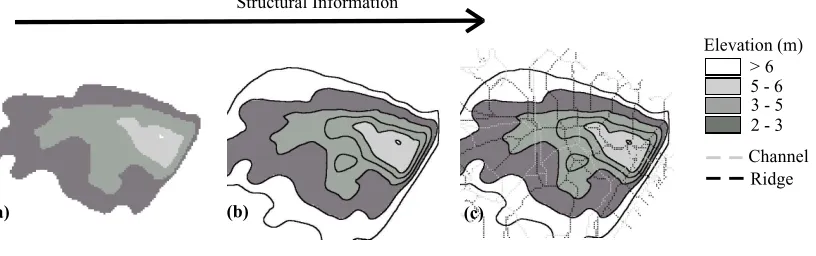
Two key information streams in a dynamic surface are the structure of the surface and the

local importance of points. In the most common representations of surfaces such as the colour

map and contour map, the delivery of the structural information is subjective to the contour

interval, spatial resolution and thematic resolution (Bajaj and Schikore, 1996).

Fowler and Little (1979) proposed that the fundamental morphometric feature networks

of a surface, constructed by connecting the peaks to passes with ridges and the pits to passes

with channels, are sufficient to describe the significant information about a surface. Later,

Helman and Hesselink (1991) and Bajaj and Schikore (1996) demonstrated that the

morphometric feature representation could enhance the visualisation of vector and scalar

surfaces significantly as compared to the colourmaps and contour maps. We suggest that the

re-expression of dynamic surfaces as morphometric feature networks will improve the grasp

of information flow in a dynamic map series. To put this in the terms of the proposal of

Dransch (2000), the morphometric feature re-expression will increase the important

information, reduce the information overload, which would help in creation of a better mental

model of the dynamic processes. Bajaj and Schikore (1996) summarised the following

advantages of using morphometric feature representation of surface:

(i) Contours and Colourmaps tend to wash out the information present within the contour

intervals and class intervals respectively. However, the morphometric features will

represent both the spatial and elevation structure of the surface (Figure 4).

(ii) Morphometric features are objective and scale invariant i.e., the definition of

morphometric feature doesn’t vary with scales.We suggest that the morphometric

(i) As the definition of morphometric feature is objective they can be used to reference

and monitor changes (quantification of movement). The use of the surface network

provides a frame of reference, which could be used to track changes in the surface for

example the rate of the displacement of the ridge lines over time could indicate the

behaviour of the surface under certain conditions (earthquakes, sea-level rise )The use

of a point and line representation of surfaces makes it more easy to follow the

dynamism in a surface as the human eye is particularly suited to monitor these

motions.2.1.2.1 Extraction of the morphometric features

Geographic Information Science and Computer Science researchers have suggested various

ways of extracting the peaks, pits, passes, ridges and channels. Wood (1996) has given a good

treatment for the various ways of extracting the topographic features. We briefly mention the

three popular methods for the classification of the points on the surface into the various

feature types:

(i) Manually by Digitising

This is the most tedious approach for the classification of the points and lines but it

remains as the final resort for the extraction of a structurally consistent (i.e., no

disconnected lines and unidentified points) set of the fundamental topographic

features from contour maps (Wolf, 1984). The automated classification of the

topographic feature suffers from a number of limitations arising out of data-specific

and algorithm-specific issues (Wood, 1998, Wood and Rana, 2000).

(ii) Triangulation

This method involves the triangulation of the surface points over a local

neighbourhood and comparing the elevations of a point with all its adjacent vertices.

The points are then classified based on this comparison (Douglas and Peucker, 1975;

Takahashi et. al., 1995).

(iii) Polynomial Surface Fitting

This method involves fitting a smooth surface through the surface points and the

points are classified based on the curvature of the fitted surface (Wood, 1998). The

advantages of using a polynomial surface fitting, specifically the bivariate quadratic

surface fitting, are described by Wood (1996, 1998).

2.1.2.2 Issues related to feature extraction

It is well known that automated raster processing suffers from the limitation that the results of

centred at the study point, used to perform the processing. This has been termed in the

literature as the scale dependency of the feature extraction (Quattrochi and Goodchild, 1996).

The topographic features exist across various scales of magnitude. While, there have been

many efforts to model the scale-space (Lindeberg, 1994) of surfaces using wavelets

(Quattrochi and Goodchild, 1996; Starck et. al, 1998), Fractals (Emerson and Quattrochi,

2000), scale-space theory (Lindeberg, 1994), Quadtrees (Csillag, 1996) to-date a unified

treatment is not agreed upon. The triangulation based feature extraction method has the

limitation that it only triangulates over a 3 points x 3 points window therefore features of a

larger magnitude may remain undetected. In contrast, the bivariate quadratic surface fitting

has the advantage that window size can be increased/decreased iteratively until a visually

acceptable level of extraction has been achieved. However, it is clear that the extraction of the

features at all the scales cannot be guaranteed.

2.1.3 Ensure periodicity and interactivity

In this proposal, our aim is to provide ways in which the information delivery can be adjusted

to data-specific and user-specific learning requirements. There is always a danger with points

and lines based dynamic maps that the duration of their display may not be suitable for

data-specific requirements (e.g., too much change displayed too much quickly) or user-data-specific

requirements (e.g., beginners). Previously, Dibiase et al. (1992) and MacEachren (1994)

proposed the use of dynamic visual variables such as moment, duration and others, which

could be used to control the information delivery pace. Openshaw et al. (1994) proposed the

idea of a progressive decay of luminosity with time until the points or symbols disappear

altogether after some fixed time. We introduce a similar capability called graphic lag

between successive events that provides more flexibility in the map interpretation process.

This has been widely in the video media as the Fading in and Fading out effect. Such a

control will provide a reference for the grasping the change, which could be useful in

observing the evolution of the map. Technically graphic lag would control the lag in time for

which a previous graphic remains on the display until the new one appears. The essential aim

of the graphic lag is to augment the working memory (Ware, 2000).For interactivity, we

propose the use of application programming environments such as Tcl/Tk (URL #3) that can

easily be coded to provide interactive graphic user interfaces (GUI) with sophisticated query

functionalities (Dykes, 1999).

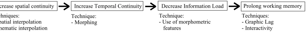
The overall flow of the implementation process in our proposal is shown in Figure 5. For the

attribute series, we decided to compare the population density of an area Northeast of

Leicester, UK, between different age groups (Figure 1). The population density surfaces are

raster of 200m spatial resolution obtained from the Small Area Statistics Dataset maintained

by the Census Dissemination Unit at the Manchester Information and Associated Services,

UK.

For the temporal series, we obtained the DEM of an active sand spit located at the

Scolt Head, Norfolk coast, UK, to model a temporal series. The point elevation data was

collected by Jonathan Raper based at City University (For a more detailed treatment of this

dataset refer to Raper, 2000) twice a year from 1992 to 1999 (Figure 2).

2.2.1 Increasing the spatial and temporal continuity

The population density surfaces of 200m spatial resolution were interpolated into 50m (i.e.,

interpolation to a higher spatial resolution) and 200m (i.e., interpolation to the existing spatial

resolution) spatial resolutions using the software LandSerf. LandSerf is a freeware developed

by Jo Wood (URL #4) provides functions for a bivariate quadratic interpolation of a raster

surface to an arbitrary spatial resolution.

The point elevation data were gridded into raster format of 6.6m spatial resolution

using Inverse Distance Weighted interpolation in the software ArcView (URL #5). This

particular spatial resolution was calculated by ArcView to be suitable to cover the geographic

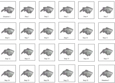
extent of the point dataset. Thereafter, the temporal gap (7 months) in each pair of

consecutive surfaces was filled with 22 intermediate surfaces by morphing the first surface in

the pair into the last surface in the pair. Morphing was done in ArcView using ArcViews’

scripting language Avenue. The user has the flexibility to specify the number of intermediate

surfaces and any number of pairs of consecutive surfaces. Perspective view of all the surfaces

was then generated using the 3D Analyst Extension in ArcView to visualise the terrain

denudation processes better. Screen grabs of a sequence of perspective grabs was then

converted into animation using the software Animation Shop (URL# 6). However, it will be

trivial to assemble all above steps into one single Avenue script in ArcView.

2.2.2 Morphometric feature extraction

The morphometric features were extracted from the population density and elevation surfaces

using the software LandSerf (URL #4). LandSerf utilises the polynomial surface fitting

extract the features defines the spatial extent of the surface’s structure yielded by the feature

extraction process. A filter size of 9 i.e., 450 m x 450 m, was used to extract the

morphometric features in the population density surfaces. In the case of elevation rasters, after

a few iterations with different filter window sizes and visual inspection a 7 x 7 window i.e.,

46.2m x 46.2m, was observed to be suitable for representing the elevation structure.

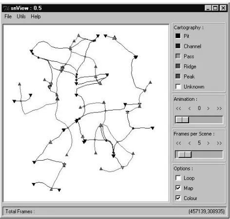
2.2.3 Graphic Lag

Graphic Lag has been implemented in an application called surface network

visualisation (SNV) (Figure 6; URL #6) developed by JD in Tcl/TK. The input in the

SNV is the morphometric feature dataset of the temporal and attribute series.

Sometimes the feature dataset, especially the ridges and channels, could have too

many vertices, which slows down the performance of the SNV. Therefore, a simple

line simplification utility has been built-in the SNV, which can downsample a ridge or

channel by skipping a user-defined number of vertices. SNV provides the flexibility to

select a user-defined graphic lag and allows querying the features, while the animation

is on display.

3. Results

3.1 Temporal Series

Figure 7 shows an example of the temporal continuity achieved by morphing the February

1997 terrain into the September 1997 terrain. While we can feel the relief changes, however it

is not possible to assess the changes in the structure of the surface, as the structure is not

obvious from the field view. Figure 8 shows a part of the same sequence of the morphing with

the overlay of the surface network, in which the changes in the structure can be spotted,

especially note the detection of the evolution of minor morphometric features in the NE

otherwise suppressed in Figure 7. The animation can be viewed at

http://www.soi.city.ac.uk/~jad7/snv/. For a more detailed discussion on the

coastal-sedimentological processes at the sand spit refer to Livingstone and Raper (1999) and Raper

et al (1999). Figure 9 shows the application of graphic lag in monitoring the splitting of the

central ridge in the sandpit with a graphic lag of? frames (can we quantify graphic lag?). As

can be clearly seen the graphic lag prolongs the working memory about the splitting of the

3.2 Attribute Series

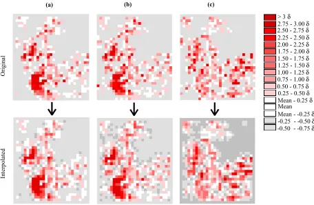
The interpolation of population density surfaces into 200m spatial resolution (Figure 10)

improves the spatial continuity from Figure 1 but the cell edges are still visible. However,

interpolation into 50m spatial resolution gives a much smoother appearance albeit it increases

the data file sizes by 4 times (Figure 11). As the morphometric feature extraction is based on

the curvature therefore, the smoother the local neighbourhood, the more reliable will be the

polynomial surface fitting. Therefore, we decided to use the 50m spatial resolution

interpolated surfaces.

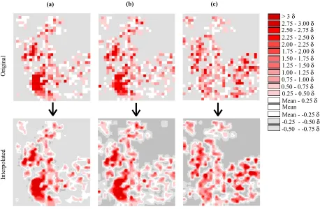
During the morphometric feature extraction, the characteristic spatial distribution of

the different age groups was revealed successfully (Figure 12). The morphometric feature

representation of the population density surfaces reveals the following interesting

observations:

- The morphometric feature networks of the 5-15 years and 60+ years age group are

generally more sparse than the 15-59 years age group.

- Some of the local population density peaks suppressed in the colour maps (Figure

11) are revealed by the morphometric feature representation. For example see the

cluster of points in the NW quadrant with some of the highest deviation from the

average population density.

4. Conclusion and Future Work

Information visualisation is not a mathematical equation, which has fixed solution domain.

One could solve mathematical equations in many ways but all the methods have to achieve an

exactly same result. The definition of information lies in the “eye of the beholder”. Therefore,

we believe (at least SR does), a good information visualisation method will always be judged

based on its qualities for a particular application. Therefore, it would be most fruitful to

combine visualisation methods employed in various disciplines to propose a working model.

Dynamic maps are perhaps the most abused forms of cartographic representations

especially now with the availability of inexpensive sophisticated hardware and software (data

and applications). It may sound daring but we would like to pose the question that does an

average human has the physical capability to fully understand a dynamic maps, especially

with our limited cognitive capabilities for parallel processing?

However, getting back to our work, generally, there is a lack of guidance on the

optimal exploitation of animated maps. We, with the examples of two types of animated

- Use of morphometric data derivatives to attract user’s attention and objective

visualisation - This achieves to attract user’s attention.

- Increasing/Enhancing the spatial/temporal autocorrelation – This helps to maintain the

attention. Use of Graphic Lag for providing more ways of feeding user’s attention time

span – This allows the user-defined flexibility in the attention span.

It is difficult to conclude on the advantages so we have left our ideas the WEB

CARTOGRAPHY FORUM (URL #8) for a field test. As part of future work, we anticipate to

work on improving the interactivity of SNV with functionalities such as the addition of colour

graphic lags, zooming in a particular part of the map during animation and others.

Acknowledgements

Thanks to Jonathan Raper for giving us the point elevation data of Scolt Head. Any

References

Bajaj, C., and Schikore, D.R., 1996. Visualization of scalar topology for structural

enhancement. Technical Report CSD-TR-96-006, Department of Computer Sciences, Purdue

University.

Bertin, J., 1967. Semiologie Graphique. Den Hagg: Mouton.

Bracken, I., 1994. Towards improved visualization of socio-economic data, In: H. M.

Hearnshaw and D. J. Unwin (Editors) Visualization in Geographical Information Systems,

Wiley and Sons, Chichester, 76-84

Csillag, F., 1996. Quadtrees: Hierarchical Multiresolution Data Structures for Analysis of

Digital Images. In: D. A. Quattrochi and M. F. Goodchild (Eds.), Scale in Remote Sensing

and GIS, Lewis Publishers: Boca Raton, Fla., 247-272.

Dibiase, D., MacEchren, A.M., Krygier, J.B., Reeves, C., 1992. Animation and the role of

map design in scientific visualization. Cartography and Geographic Information Systems, 19

(4), 201-204.

Douglas, D. and T. K. Peucker, 1975, "Detection of surface-specific points by local parallel

processing of discrete terrain elevation data". Computer graphics, Visions and Image

Processing, Vol. 4, No. 2, pp. 375-387.

Dransch, D., 2000. The use of different media in visualizing spatial data, Computers and

GeoSciences, v. 26(4), 5-9

Dykes, J.A., 1999. Scripting Dynamic Maps: Some Examples and Experiences with Tcl/Tk,

in Cartwright, W., Peterson, M.P. & Gartner, G., Multimedia Cartography, Springer-Verlag,

Berlin, 195-204.

Earnshaw, R.A., and Watson, D., 1993. Animation and scientific visualization: tools and

applications. Academic Press: London ;San Diego.

Emmer, N.N.M., 2001. Determining the effectiveness of animations to represent geo-spatial

Information Science, Association of Geographic Information Laboratories in Europe. Brno,

585-589.

Emerson, C.W., and Quattrochi, D.A., 2000. Applications of fractal analytical techniques in

the estimation of operational scale, Proceedings IAPRS, v. XXXIII, Amsterdam, Netherlands.

Fowler, R. J., Little, J.J, 1979. Automated extraction of irregular network digital terrain

models. Computer Graphics 13,199 - 207.

Gahegan, M., 1999. Four barriers to the development of effective exploratory visualisation for

the geosciences. International Journal of Geographical Information Science, 13(4), 289-309.

Gatrell, A., 1994. Density estimation and the visualization of point systems, In: H. M.

Hearnshaw and D. J. Unwin (Editors) Visualization in Geographical Information Systems,

Wiley and Sons, Chichester, 65-75

Gomes, J., Costa, B., Darsa, L., and Velho, L., 1999. Warping & Morphing of Graphical

Objects, Morgan Kaufman, 490 pp

Hayward, S., 1984. Computers for animation. Page Bros.: Norwich, UK.

Helman, J.L., and Hesselink, L., 1991. Visualizing Vector Field Topology in Fluid Flows.

IEEE Computer Graphics and Applications, 11(3), 36-46.

Koussoulakou, A., 1990. Computer-assisted cartography for monitoring spatio-temporal

aspects of urban air pollution. PhD Thesis, Delft Press: University of Delft, Netherlands.

Kreuseler, M., 2000. Visualization of geographically related multidimensional data in virtual

3D scenes, Computers and GeoSciences, v. 26, 101-108

Lindeberg, T., 1994. Scale-space Theory in Computer Vision. Kluwer Academic Press:

Dordrecht.

Livingstone, D.L., and Raper, J.F., 1999. Developing a visualisation system for simulating the

Livingstone, D.L., Raper, J.F., and McCarthy, T.M., 1999. Integrating aerial videography and

digital photography with terrain modelling. Geomorphology, 29(1), 77-92.

MacEchren, A.M., 1994. How Maps Work: Issues in Representations and Design, Guildford

Press: New York.

McCloud, S., 1993, Understanding comics. Kitchensink Press: Northampton, USA.

Mitas, L., and Brown, W.M., and Mitasova, H. , 1997. Role of dynamic cartography in

simulations of landscape processes based on multi-variate fields. Computers and Geosciences,

23(4), 437-446.

Morse, S.P., 1968. A Mathematical Model for the Analysis of Contour-Line data. Journal of

the Association for Computing Machinery, 205 – 220.

Morse, S.P., 1969. Concepts of Use in Contour Map Processing. Communications of the

Association for Computing Machinery, 147 – 152.

Ogao, P.J. and C.A. Blok, 2001. Cognitive aspects on the representation of dynamic

environmental phenomena using animations. In: C. Rautenstrauch and S. Patig (Eds).

Environmental Information Systems in Industry and Public Administration, Idea Group

Publishers, USA,13-24.

Ogao, P.J. and Kraak, M-J., 2001. Geospatial data exploration using interactive and intelligent

cartographic animations. Proceedings of the International cartographic conference, August

Beijing, China.

Openshaw, S., Waugh, D., and Cross, A., 1994. Some ideas about the use of map animation

as a spatial analysis tool. In: H. M. Hearnshaw and D. J. Unwin (Editors) Visualization in

Geographical Information Systems, Wiley and Sons, Chichester, 131-138.

Paddenburg, A.V. and Wachowicz, M., 2001. The effect of generalisation on filtering noise

for spatio-temporal analyses

Peterson, M.P., 1993. Interactive cartographic animation. Cartography and GIS, 20(1), 40-44.

Pfaltz, J.L., 1978. Surface Networks, An Analytic Tool for the study of Functional Surfaces.

Final Report NSF Grant DCR-74-13353, Department of Applied Math and Computer

Science, University of Virginia.

Quattrochi, D.A. and Goodchild, M.F., 1996. Scale in Remote Sensing and GIS. Lewis

Publishers: Boca Raton, Fla.

Slocum, T.A., Robeson, S.H., Egbert, S.L., 1990. Traditional versus sequenced choropleth

maps: an experimental investigation. Cartographica, 27(1), 67-88.

Stark, J.L., Murtagh, F., and Bijaoui, A., 1998. Image Processing and Data Analysis – The

Multiscale Approach, Cambridge University Press: Cambridge.

Ware, C., 2000. Information Visualisation: Perception for Design, Morgan Kaufmann, CA, p.

368

Werner, C., 1988. Formal Analysis of Ridge and Channel Patterns in Maturely Eroded

Terrain. Annals of the Association of American Geographers, 253-270.

Takahashi, S., Ikeda, T., Shinagawa, Y., Kunii, T.L., and Ueda, M., 1995. Algorithms for

Extracting Correct Critical Points and Constructing Topological Graphs from Discrete

Geographical Elevation Data. The International Journal of the Eurographics Association, 14

(3), C-181- C-192.

Tobler, W.R., 1970. A computer movie simulating urban growth in the Detroit region,

Economic Geography, 46, 234 - 240

Whigham, P., 2001. Spatial Information: Problems, Challenges and Directions. Key Note

Lecture at the GeoComputation 2001 September 24 -26, University of Queensland, Australia.

Wolf, G.W., 1984. A mathematical model of cartographic generalization. Geo-Processing, 2

(3), 271-286.

Wood, J.D., 1996. The geomorphological characterisation of Digital Elevation Models. PhD

Wood, J.D., 1998. Modelling the continuity of Surface form using Digital Elevation Models.

In: Proceedings 8th International Symposium on Spatial Data Handling, Vancouver, Canada, 725-736.

Wood, J., and Rana, S., 2000, Construction of Weighted Surface Networks for the

Representation and Analysis of Surface Topology, In: Proceedings Geocomputation 2000

August 23 -25, University of Greenwich, UK.

URLS:

1. http://census.ac.uk/cdu/surpop/background.html

2. http://www.discreet.com

3. http://www.scriptics.com

4. http://www.soi.city.ac.uk/~jwo/landserf/

5. http://www.esri.com

6. http://www.jasc.com

7. http://www.soi.city.ac.uk/~jad7/snv/

> 3 δ 2.75 - 3.00 δ Population Density

2.25 - 2.50 δ

1.75 - 2.00 δ

0.25 - 0.50 δ 1.25 - 1.50 δ

Mean 0.75 - 1.00 δ

-0.25 - -0.50 δ 2.50 - 2.75δ

2.00 - 2.25 δ

1.50 - 1.75 δ

Mean - 0.25 δ 1.00 - 1.25 δ

Mean - -0.25 δ 0.50 - 0.75 δ

-0.50 - -0.75 δ

(a) (b) (c)

Figure 1. Population density surfaces of an area in NE Leicestershire. (a) 5-15 years (b) 15-59 years (c) 60-60+ years. The rasters have been classified in 1/4 standard deviation classes.

To same spatial resolution Original surface with a data value

Interpolated surface with a data value

To higher spatial resolution

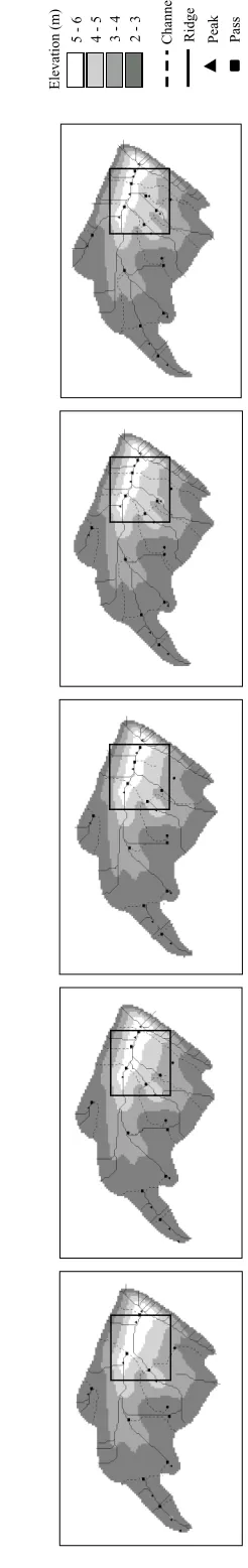
Figure 3. Digital elevation models of a sand spit at Scolt Head, Norfolk coast during (a) February, 1997 and (b) September, 1997.

?

Elevation (m)

3 - 5 2 - 3

Figure 4. Increase in the structural information delivery with the addition of (a) Raster colour map of a part of Scolt Head sand spit, (b) Contour map of (a), and (c) Morphometric features in the sand spit.

morphometric features.

> 6 5 - 6

Channel Ridge Structural Information

Elevation (m)

3 - 5 2 - 3

Figure 5 Proposed implementation of techniques to augment the visualisation of dynamic raster surfaces

Increase spatial continuity

Techniques:

- Spatial interpolation - Thematic interpolation

Technique: - Morphing

Techniques: - Graphic Lag - Interactivity Technique:

- Use of morphometric features

Prolong working memory Decrease Information Load

Figure 7. 22 Intermediate surfaces (microsteps) generated by blending the February, 1997 surface (Situation 1) into the September, 1997 (Situation 2) surface.

Situation 2 Step 6

Step 12

Step 18 Step 19

Step 13 Step 14

Step 7 Step 8 Step 9 Step 10 Step 11

Situation 1 Step 1 Step 2 Step 3 Step 4 Step 5

Step 15 Step 16 Step 17

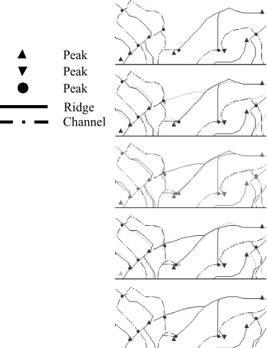
Figure 8. Use of the morphometric features to highlight the changes in the morphometry of the sand spit. A box is used to indicate an area of interest. Note that the morphometric features identify changes that are not evident from the representation that uses color to show variation in elevation.

time

5 - 6 4 - 5 Channel Ridge Peak Pass Pit

Elevation (m)

Frame 1: initial state shows a split ridge (centre of frame - see key) with bifurcation. This is the main feature in the sand bar.

Frame 2: a light outline of the network associated with the subsequent event is added ensuring visual smoothing

Frame 3: the network associated with the first event is lightened whilst that of the subsequent event is darkened

Frame 4: the process continues with the subsequent event clearly showing the development of an additional bifurcation: a discernable ridge joining two other ridge features

Frame 5: all evidence of the initial event is removed. The process continues between successive frames in the animation.

Figure 9. Use of the graphic lag to the highlight the changes in the Scolt Head dynamic sand spit.

Figure 10. Interpolation of the NE Leicestershire population density surfaces to 200 m spatial resolution. (a) 5-15 years (b) 15-59 years (c) 60-60+ years. The rasters have been classified in 1/4 standard deviation classes.

> 3 δ 2.75 - 3.00 δ

O

ri

gi

na

l

In

te

rpol

at

ed

2.25 - 2.50 δ

1.75 - 2.00 δ

0.25 - 0.50 δ 1.25 - 1.50 δ

Mean 0.75 - 1.00 δ

-0.25 - -0.50 δ 2.50 - 2.75δ

2.00 - 2.25 δ

1.50 - 1.75 δ

Mean - 0.25 δ 1.00 - 1.25 δ

Mean - -0.25 δ 0.50 - 0.75 δ

-0.50 - -0.75 δ

> 3 δ 2.75 - 3.00 δ

O

ri

gi

na

l

In

te

rpol

at

ed

2.25 - 2.50 δ

1.75 - 2.00 δ

0.25 - 0.50 δ 1.25 - 1.50 δ

Mean 0.75 - 1.00 δ

-0.25 - -0.50 δ 2.50 - 2.75δ

2.00 - 2.25 δ

1.50 - 1.75 δ

Mean - 0.25 δ 1.00 - 1.25 δ

Mean - -0.25 δ 0.50 - 0.75 δ

-0.50 - -0.75 δ

(a) (b) (c)

> 3 δ 2.75 - 3.00 δ

O ri gin al In te rp o lat ed M o rphom et ri c F ea tu re s

2.25 - 2.50 δ

1.75 - 2.00 δ

0.25 - 0.50 δ 1.25 - 1.50 δ

Mean 0.75 - 1.00 δ

-0.25 - -0.50 δ 2.50 - 2.75δ

2.00 - 2.25 δ

1.50 - 1.75 δ

Mean - 0.25 δ 1.00 - 1.25 δ

Mean - -0.25 δ 0.50 - 0.75 δ

-0.50 - -0.75 δ

(a) (b) (c)

Channel Ridge Peak Pass Pit