Forecasting time series with complex seasonal patterns using exponential smoothing

Department of Econometrics and Business Statistics

Forecasting time series with

complex seasonal patterns using

exponential smoothing

Alysha M De Livera and Rob J Hyndman

seasonal patterns using exponential

smoothing

Alysha M De Livera

Department of Econometrics and Business Statistics, Monash University, VIC 3800

Australia.

Email: [email protected]

Division of Mathematics, Informatics and Statistics,

Commonwealth Scientific and Industrial Research Organisation, Clayton, VIC 3168

Australia.

Email: [email protected]

Rob J Hyndman

Department of Econometrics and Business Statistics, Monash University, VIC 3800

Australia.

Email: [email protected]

seasonal patterns using exponential

smoothing

Abstract

A new innovations state space modeling framework, incorporating Box-Cox transformations, Fourier series with time varying coefficients and ARMA error correction, is introduced for forecasting complex seasonal time series that cannot be handled using existing forecasting models. Such complex time series include time series with multiple seasonal periods, high frequency seasonality, non-integer seasonality and dual-calendar effects. Our new modelling framework provides an alternative to existing exponential smoothing models, and is shown to have many advantages. The methods for initialization and estimation, including likelihood evaluation, are presented, and analytical expressions for point forecasts and interval predictions under the assumption of Gaussian errors are derived, leading to a simple, comprehensible approach to forecasting complex seasonal time series. Our trigonometric formulation is also presented as a means of decomposing complex seasonal time series, which cannot be decomposed using any of the existing decomposition methods. The approach is useful in a broad range of applications, and we illustrate its versatility in three empirical studies where it demonstrates excellent forecasting performance over a range of prediction horizons. In addition, we show that our trigonometric decomposition leads to the identification and extraction of seasonal components, which are otherwise not apparent in the time series plot itself.

Keywords: exponential smoothing, Fourier series, prediction intervals, seasonality, state space models, time series decomposition.

1

Introduction

Many time series exhibit complex seasonal patterns. For example, Figure1(a) shows the number of retail banking call arrivals per 5-minute interval between 7:00am and 9:05pm each weekday. There is a daily seasonal pattern with frequency 169 and a weekly seasonal pattern with frequency 169_×5=845. If a longer series of data were available, there may also be an annual seasonal pattern. Such multiple seasonal patterns are becoming more common with high frequency data recording. Further examples where multiple seasonal patterns can occur include daily hospital admissions, requests for cash at ATMs, electricity and water usage, and access to computer web sites.

Other time series (most commonly weekly data) have patterns with a non-integer frequency. Fig-ure1(b) shows the weekly United States finished motor gasoline products in thousands of barrels per day. The time series clearly exhibits an annual seasonal pattern with frequency 365.25/7≈52.179. In addition, some time series may have dual-calendar seasonal effects. Figure1(c) shows the daily electricity demand in Turkey over nine years, from 1 January 2000 to 31 December 2008. A clear weekly seasonal pattern and an annual seasonal pattern can be observed in the time series. The annual seasonality consists of two separate seasonal patterns with frequencies of 354.37 and 365.25, following the Hijri and Gregorian calendars respectively. The Islamic Hijri calendar is based on lunar cycles and is used for religious activities and related holidays. It is approximately 11 days shorter than the Gregorian calendar. The Jewish, Hindu and Chinese calendars create similar effects that can be observed in time series affected by cultural and social events (e.g., electricity demand, water usage, and other related consumption data), and need to be accounted for in forecasting studies (Lin & Liu 2002,Riazuddin & Khan 2005). Unlike the multiple periodicities seen with hourly and daily data, these dual calendar effects involve non-nested seasonal periods.

Most existing time series models are designed to accommodate simple seasonal patterns with a small integer-valued periodicity (such as 12 for monthly data or 4 for quarterly data). There are a few models which attempt to deal with more complex seasonal patterns (e.g.,Harvey & Koopman(1993),

Harvey et al.(1997),Pedregal & Young(2006),Taylor(2003b),Gould et al.(2008),Taylor & Snyder

(2009),Taylor(2009)), but none that is able to handle all of the complexities above.

In this paper we introduce a new innovations state space modeling framework based on a trigono-metric formulation which is capable of tackling all of these seasonal complexities. Using the above time series, we show that these trigonometric exponential smoothing models provide exceptional

100

200

300

400

5 minute intervals

Number of call arrivals

3 March 17 March 31 March 14 April 28 April 12 May

(a)Number of call arrivals handled on weekdays between 7am and 9:05pm from March 3, 2003, to

May 23, 2003 in a large North American commercial bank.

6500 7000 7500 8000 8500 9000 9500 Weeks

Number of barrels (Thousand barrels per day)

1991 1993 1995 1997 1999 2001 2003 2005

(b)US finished motor gasoline products supplied (thousands of barrels per day), from February 1991

to July 2005. 10000 15000 20000 25000 Days Electricity demand (MW) 2000 2001 2002 2003 2004 2005 2006 2007 2008

(c)Turkish electricity demand data from January 1, 2000, to December 31, 2008.

out-of-sample forecasting performances and offer an elegant decomposition of complex seasonal time series.

In Section 2 we discuss the existing exponential smoothing models, their weaknesses and their inadequacy in handling complex seasonal patterns, and present a modified, generalized modeling framework in order to overcome these problems. We then introduce in Section3the new trigono-metric innovations state space modeling framework, which is capable of handling complex seasonal patterns, as well as the usual single seasonal patterns, in a straightforward manner with fewer parameters. Section4describes both analytical and simulated prediction distributions, as well as point and interval predictions for the models. Section5presents the methods used for initialization and estimation, including the derivation of maximum likelihood estimators and the methodology used in applying the models. In Section6, we explain the trigonometric formulation as a way of decomposing complex seasonal time series, which cannot be decomposed using any of the existing decomposition techniques. The proposed models are then applied to the US gasoline products data, the call center data and the Turkey electricity demand data in Section7, and it is shown that these new trigonometric exponential smoothing models provide outstanding forecasting performances over a range of forecasting horizons, compared to the existing models. Furthermore, using these applica-tions, we demonstrate the decomposition of complex seasonal time series using our trigonometric approach. Some conclusions are drawn in Section8.

2

Exponential smoothing models for seasonal data

2.1 Traditional models

Single seasonal exponential smoothing methods are among the most widely used forecasting pro-cedures in practice (Snyder et al. 2002,Makridakis et al. 1982,Makridakis & Hibon 2000). These methods have been shown to be optimal for a class of innovations state space models (Ord et al. 1997,

Hyndman et al. 2002), thus allowing a stochastic modelling framework for exponential smoothing including likelihood calculation, prediction intervals, model selection, and so on. The single source of error or innovations approach is known to be simple yet robust, and has been shown to have several advantages over the multiple source of error models (Ord et al. 2005,Hyndman et al. 2008). The most commonly employed seasonal models in the innovations state space modeling framework include the underlying models for the well-known Holt-Winters’ additive and multiplicative seasonal exponential smoothing methods. However, these models are inadequate for handling complex

seasonal time series such as multiple seasonality, non-integer seasonality and dual-calender effects.

Taylor(2003b) extended the single seasonal Holt-Winters’ model to accommodate a second seasonal component in order to handle time series with two seasonal patterns. This requires a large number of values to be estimated for the initial seasonal components, especially when the frequencies of the seasonal patterns are high, which may lead to over-parameterization. Gould et al. (2008) attempted to reduce the over-parameterization of this model by dividing the longer seasonal length into sub-seasonal cycles that have similar patterns. However, this model is relatively complex and can only be used in modeling double seasonal patterns when one seasonality is a multiple of the other. Using six years of British and French electricity demand data,Taylor(2009) illustrated that extended additive seasonal versions of the above models to handle a third seasonal pattern can outperform the double seasonal exponential smoothing models. However, none of these models can be used to model complex seasonal patterns such as non-integer seasonality and calendar effects, or time series with more than two non-nested seasonal patterns.

In addition, the non-linear versions of exponential smoothing models, although widely used, suffer from some important weaknesses. Akram et al. (2009) showed that most non-linear seasonal exponential smoothing models can be unstable, having infinite forecast variances beyond a certain forecasting horizon. Of the multiplicative error models which do not have this flaw, Akram et al.

(2009) proved that sample paths will converge almost surely to zero even when the error distribution is non-Gaussian. Furthermore, for non-linear exponential smoothing models, analytical results for the prediction distributions are not available.

The models used for exponential smoothing assume that the error process is serially uncorrelated. However, the assumption of an uncorrelated error process does not always hold. In an empirical study, using the Holt-Winters’ method for multiplicative seasonality,Chatfield(1978) showed that the error process is correlated and can be described by an AR(1) process. This was further illustrated byTaylor(2003b) in a study of electricity demand forecasting using a double-seasonal Holt-Winters’ multiplicative method. Gardner(1985),Reid(1975), andGilchrist(1976) have also mentioned this issue of correlated errors, in improving the forecast accuracy.

2.2 Modified models

We now consider various modifications to the standard exponential smoothing models to enable them to handle a wider variety of seasonal patterns, and to deal with the problems raised above.

Extending non-linear exponential smoothing models to handle more than two seasonal patterns may make these models unnecessarily complex, and the estimation and model selection procedure may become cumbersome. Also, the problems with non-linear models that are noted above are also a problem in any extended versions. Consequently, rather than allow non-linear forms, we restrict attention to linear homoscedastic models but allow some types of non-linearity using Box-Cox transformations (Box & Cox 1964). The notation y_t(ω)is used to represent Box-Cox transformed observations with the parameterω, where ytis the observation at timet.

We can extend exponential smoothing models to accommodateT seasonal patterns as follows.

y_t(ω)=    y_tω−1 ω ; ω6=0 logyt ω=0 y_t(ω)=`t−1+φbt−1+ T X i=1 s(<sub>t</sub>i<sub>−</sub>)<sub>m</sub> i +dt `t=`t−1+φbt−1+αdt (1) b_t=φb_t−1+βdt s(_ti)=s(_ti₋)_m i +γidt dt= p X i=1 ϕidt−i+ q X i=1 θi"t−i+"t,

wherem1, . . . ,mT denote the seasonal periods,`t and bt represent the level and trend components

of the series at timet, respectively,s(_ti)represents theith seasonal component at time t,d_t denotes an ARMA(p,q) process and "_t is a Gaussian white noise process with zero mean and constant varianceσ2. The smoothing parameters are given byα,β,γ_ifori=1, . . . ,T, andφis the dampening parameter, which gives more control over trend extrapolation when the trend component is damped (Hyndman et al. 2002,Taylor 2003a).

The notation BATS(p,q,m1,m2, . . . ,mT) is used for these models. B stands for the Box-Cox

trans-formation, A stands for the ARMA residuals, T stands for the trend component in the model and S stands for the seasonal components. The arguments indicate the ARMA parameters (p and q) and the seasonal periods (m1, . . . ,mT). For example, BATS(0, 0,m1) with φ =1 andω=1

rep-resents the underlying model for the well-known Holt-Winters’ additive single seasonal method. The double seasonal Holt-Winters’ additive seasonal model described byTaylor(2003b) is given by BATS(0, 0,m1,m2) withφ=1 andω=1, and that with the residual AR(1) adjustment in the model

ofTaylor(2003b,2008) is given by BATS(1, 0,m1,m2). The Holt-Winters’ additive triple seasonal

model with AR(1) adjustment inTaylor(2009) is given by BATS(1, 0,m₁,m₂,m₃).

The BATS model is the most obvious generalization of the traditional exponential smoothing models to allow for multiple seasonal periods. However, it is not capable of handling non-integer seasonality, and it suffers from a very large number of parameters that require estimation; the initial seasonal component alone containsm1+m2+· · ·+mT parameters. This becomes a huge number of values

when the frequencies of the seasonal patterns are high. For example, for the call center data shown in Figure1(a), 169+845=1014 initial seasonal values must be estimated.

3

Trigonometric exponential smoothing models for seasonal data

Consequently, we introduce a new trigonometric representation of seasonal components based on Fourier series. We could replace the equation fors(_ti)in the BATS model with

s(_ti)= ki X j=1 α(i) j,tcos(λ (i) j t) +β (i) j,tsin(λ (i) j t) (2a) α(i) j,t=α (i) j,t−1+κ (i) 1 dt (2b) β(i) j,t =β (i) j,t−1+κ (i) 2 dt, (2c)

whereκ(₁i)andκ(₂i)are the smoothing parameters andλ(_ji)=2πj/m_i. This is an extended, modified single source of error version of a single seasonal multiple source of error representation suggested byHannon et al.(1970), and is equivalent to index seasonal approaches when ki=mi/2 for even

values ofm_i, and whenk_i= (m_i−1)/2 for odd values ofm_i. But most seasonal terms will require much smaller values ofk_i, thus reducing the number of parameters to be estimated.

In the single seasonal multiple source of error setting (Harvey 1989), an alternative, but equivalent formulation of representation (2) is preferred (Durbin & Koopman 2001), which can be obtained by re-parameterizing the single seasonal multiple source of error version of (2) using

α(i) j,t=s (i) j,tcos(λ (i) j t)−s ∗(i) j t sin(λ (i) j t)

For our modified multiple seasonal single source of error formulation, it can be shown (see Ap-pendixA) that the above re-parametrization leads to the following:

s(_ti)=

ki

X

j=1

s(_ji_,)_t, (3)

where s(_ji_,t)=s(_j,i_t)₋₁cosλ(_ji)+s∗_j,(_ti₋)₁sinλ(_ji)+hκ₁(i)cos(λ(_ji)t) +κ(₂i)sin(λ(_ji)t)id_t s∗_{j t}(i)=−sj,t−1sinλ( i) j +s ∗(i) j,t−1cosλ (i) j + h κ(i) 2 cos(λjt)−κ( i) 1 sin(λjt) i dt

This then gives rise to a heteroscedastic error process. However, to be consistent with the homoscedas-tic nature of the traditional additive innovations state space models, the following representation is employed in our models:

s(_ti)= ki X j=1 s(_ji_,)_t (4a) s(_ji_,)_t=s(_ji_,)_t−1cosλ(_ji)+s∗_j,(_ti₋)₁sinλ(_ji)+γ(₁i)d_t (4b) s∗_{j t}(i)=−sj,t−1sinλ(_ji)+s∗_j,(ti−)1cosλ (i) j +γ (i) 2 dt. (4c)

In the single seasonal multiple source of error setting, (2) is equivalent to (4) (Proietti 2000). In our multiple seasonal single source of error setting, the seasonal representations (2) and (4) are equivalent only when the smoothing parameters are equal to zero. This then reduces to a standard Fourier series representation when the initial state values s(_ji_,0) and s∗_j,0(i) are set to Fourier series coefficients for theith seasonal component. Then, followingKoopman & Lee(2005), it can be shown thats∗_{j t}(i)= 1 λ(i) j ds(_ji_,)_t d t . Thuss ∗(i)

j t is proportional to the rate of growth ins (i)

j,tfor each seasonal component.

Hence, in the representation (4), the terms(_ji_,)_tcould be defined as the stochasticlevelterm of theith seasonal component and the terms∗_{j t}(i)as a stochasticauxiliaryvariable describing the growth in the

levelof the ith seasonal component that is needed to describe the change in the seasonal component over time.

Replacing the seasonal component s(_ti) in (1) with that given by (4), a new class of exponential smoothing models, termedtrigonometric exponential smoothing models, is obtained. The notation TBATS(p,q,_{m1,k1},{m2,k2}, . . . ,{mT,kT}) is used for these trigonometric models. These models

require the estimation of 2(k1+k2+· · ·+kT)initial seasonal values, which is expected to greatly

reduce the number of parameters required compared to BATS models. The use of trigonometric functions also allows the modelling of non-integer seasonal frequencies.

4

Point forecasts, prediction distributions and interval

predic-tions

The BATS and TBATS models can be written in the following linear innovations state space form:

y_t(ω)=w0x_t−1+"_t (5a)

x_t=F x_t−1+g"_t, (5b)

wherew0is a row vector,g is a column vector,F is a matrix andx_t is the unobserved state vector at timet.

To obtain the matrices in (5a), we first define ˜s_t(i)= (s_1,(i)_t,s_2,(i)_t, . . . ,s(_ki)

i,t), ˜s ∗(i) t = (s∗( i) 1,t ,s ∗(i) 2,t , . . . ,s ∗(i) ki,t), s_t(i)= (˜s_t(i),˜s_t∗(i))0; let1_r= (1, 1, . . . , 1)and0_r= (0, 0, . . . , 0) be row vectors of length r; letγ(₁i)=

γ(i) 1 1ki, γ (i) 2 =γ( i) 2 1ki, γ (i)_{= (γ}(i) 1 ,γ( i) 2 )0, ϕ= (ϕ1,ϕ2, . . . ,ϕp)andθ= (θ1,θ2, . . . ,θp); letOu,v be a

u×vmatrix of zeros, letI_u,v be au×vrectangular diagonal matrix with element 1 on the diagonal, and leta(i)= (1_k

i,0ki)

0_{. We shall also need the matrices}

B=       γ(1)_ϕ .. . γ(T)_ϕ       , C =       γ(1)_θ .. . γ(T)_θ       , A_i =    C(i) S(i) −S(i) C(i)   , ˜ A_i=    0_m i−1 1 I_m i−1 0 0 mi−1   , and A=LT

i=1Ai, whereC(i) and S(i) are ki ×ki diagonal matrices with elements cos(λ( i)

j ) and

sin(λ(_ji)), respectively, for j=1, 2, . . . ,k_i and i=1, . . . ,T, and whereL

denotes the direct sum of the matrices. Letτ=2P_iT₌₁ki.

Then the TBATS model can be written in the form (5a) with

x_t=`_t,bt,s( 1) t 0 , . . . ,s_t(T)0,dt,dt−1, . . . ,dt−p+1,"t,"t−1, . . . ,"t−q+1 0 w= 1,φ,a(1)0, . . . ,a(T)0,ϕ,θ 0 g =α,β,γ(1)0, . . . ,γ(T)0, 1,0_p−1, 1,0q−1 0

and F =                   1 φ 0_τ αϕ αθ 0 φ 0_τ βϕ βθ 00_τ 00_τ A B C 0 0 0_τ ϕ θ 00_p−1 00_p−1 O_p−1,τ Ip−1,p Op−1,q 0 0 0_τ 0_p 0_q 00_q−1 00_q−1 O_q−1,τ Oq−1,p Iq−1,q                   .

These matrices are for the TBATS model when all of the components are present in the model. When a component is omitted, the corresponding terms in the matrices must be omitted.

The state space form of the BATS model can be obtained by lettings_t(i)= (s(_ti),s(_ti₋)₁, . . . ,s(_ti₋)_(m

i−1)) 0_, a(i)= (0_m i−1, 1) 0_{, γ}(i) _{= (γ} i,0mi−1) 0_{, A=}LT

i=1A˜i, and by replacing 2ki with mi in the matrices

presented above for the TBATS models.

Let ϑ be a vector of all parameters to be estimated in the model, consisting of the smoothing parameters and the Box-Cox parameter, and letnbe the length of the time series,hthe length of the forecast horizon, and yn+h|n≡ yn+h|xn,ϑthe prediction distribution of a future value of the series

given the model, its estimated smoothing parameters and the state vector at the last observation. A Gaussian assumption for the errors implies that y_n(ω₊)_h|n is also normally distributed, with mean E(y_n(ω₊)_h|n)and variance V(y_n(ω₊)_h|n)given by the equations (Hyndman et al. 2005):

E(y_n(ω₊)_h|n) =w0Fh−1x_n (6a) V(y_n(ω₊)_h|n) =      σ2 _ifh=1; σ2 – 1+ h−1 X j=1 c2_j ™ ifh_≥2; (6b)

where c_j = w0Fj−1g. Point forecasts and forecast intervals may be obtained using the inverse Box-Cox transformation. Point forecasts obtained this way are equal to the median of the conditional probability density of y_n+h|n. Forecast intervals retain the required probability coverage under back-transformation because the Box-Cox transformation is monotonic.

5

Estimation and model selection

5.1 Maximum likelihood estimation

The Box-Cox parameter and smoothing parameters,ϑ, and the initial states, x₀, can be estimated from the observed data y= (y₁, . . . ,y_n)by maximizing the likelihood. If"_t∼N(0,σ2)and x₀ andϑ are known, then y_t(ω)∼N(w0x_t−1,σ2). Thus,

p(y(_tω)|x0,ϑ) = n Y t=1 p(y(_tω)|x_t−1,ϑ) = n Y t=1 p("_t) = 1 (2πσ2)n2 exp −1 2σ2 n X t=1 "2 t ! and so p(y_t|x0,ϑ) =p(yt(ω)|x0,ϑ) det ‚ ∂y_t(ω) ∂y Œ =p(y_t(ω)|x0,ϑ) n Y t=1 y_tω−1 = 1 (2πσ2)n2 exp −1 2σ2 n X t=1 "2 t ! _n Y t=1 y_tω−1.

Therefore, the log likelihood is given by

L = −n 2 log(2πσ 2₎ − Pn t=1" 2 t 2σ2 + (ω−1) n X t=1 logyt. (7)

The maximum likelihood estimate of the error variance is obtained by letting the partial derivative of

L with respect toσ2be equal to zero, giving

ˆ σ2_=n−1 n X t=1 "2 t (8)

Then, substituting (8) into (7), multiplying by₋2, and omitting constant terms, we obtain

L∗(ϑ,x₀) =nlog ‚ _n X t=1 "2 t Œ −2(ω₋1) n X t=1 logy_t. (9)

This quantity can be minimized to obtain maximum likelihood estimates.

To start the optimization, we need some initial estimates ofx₀andϑ. If a Box-Cox transformation is required for the data, an initial value for the Box-Cox parameterωhas to be approximated first. This could be done by inspection of the data under different transformations or simply by lettingω=0 to start with. (We found this choice led to better model selection and forecasting than other initial

Let m∗ =bmax(m1, . . . ,mT)c. Then we compute a 2×m∗ moving average through the first few

seasons of transformed data. Denote this by_{f_t}(t=m∗/2+1,m∗/2+2, . . .), and letz_t =y_t(ω)₋f_t. For TBATS models, the seasonal component is then approximated using

z_t≈ T X i=1 ki X j=1 a(_ji)cos(λ(_ji)t) +b(_ji)sin(λ(_ji)t), (10)

whereaˆ(_ji)andˆb(_ji)are estimated by regressingztagainst the trigonometric terms. The initial seasonal

states for theith seasonal component can then be set toaˆ(_ji)andˆb(_ji). For BATS models, we follow the same procedure but replaceki withmi/2 for even frequencies and(mi−1)/2 for odd frequencies in

equation (10), in order to obtainaˆ(_ji)andˆb(_ji). Using these values, we define the initial seasonal state estimates aszˆ(_ti)=Pki j=1 h ˆ a(_ji)cos(λ(_ji)t) + ˆb(_ji)sin(λ(_ji)t) i .

The initial level and trend components can be approximated by computing a linear regression on the firstm∗deseasonalized values, against a time variablet=1, . . . ,m∗. Then set the initial level to be the intercept of this regression and let the initial trend be equal to the slope. For BATS models with

T=1, this is equivalent to the procedure proposed byHyndman et al.(2002).

These initial state values can then be optimized along with the Box-Cox parameter and the smoothing parameters. In practice, the initial seasonal states can only be optimized when there are a small number of values. For this reason, when handling high frequency data, the initial seasonal values can not be optimized in the BATS model. One of the advantages of the TBATS model is that there are fewer initial seasonal values, and hence the initial seasonal states may be optimized.

For the BATS model, the seasonal values are constrained when optimizing, so that each seasonal component sums to zero. For both models, using the matrices and vectorsD,g andw from equation (5a), the smoothing parameters are restricted to theforecastibility regiongiven byHyndman et al.

(2007). Restricting the parameters in this way, rather than restricting them to the usual parameter region of [0, 1], serves two purposes. First, it guarantees stable forecasts. Second, if the usual parameter region lies within the forecastibility region, then restricting the parameters to the usual region may lead to inferior forecasts as the maximum likelihood parameters may lie outside that region. In addition, ARMA coefficients are restricted to the causality and invertibility regions.

5.2 Model selection

In this paper, the AIC=_L∗( ˆϑ,xˆ₀)+2Kis used for choosing between the models, whereKis the total number of parameters inϑplus the number of free states inx , andϑˆandˆx denote the estimates

ofϑandx₀. When one of the smoothing parameters takes the boundary value 0, the value ofK is reduced by one as the model simplifies to a special case. For example, ifβ=0, then b_t=b₀for allt. Similarly, when eitherφ=1 orω=1, the value ofKis reduced by one in each instance to account for the resulting simplified model.

In an empirical study,Billah et al.(2005) indicated that information criterion approaches, such as the AIC, provide the best basis for automated model selection, relative to other methods such as the prediction-validation method. Alternative information criteria such as the AICc or BIC (Burnham & Anderson 2002) may also be used.

Selecting the number of harmonics k_i in the trigonometric models

The forecasts from the TBATS model depend on the number of harmonicsk_i used for theith seasonal component. It would be impractical to consider all possible combinations when searching for the optimalk_icombination. Instead, the following procedure was used to obtain the number of harmonics for the applications in this paper. In practice we have found that this approach leads to good models and further computational effort rarely leads to much improvement.

Using the first few seasons, we use multiple linear regression applied to (10) to find the trigonometric coefficients. Starting with a single harmonic, we gradually add harmonics, testing the significance of each one usingF-tests. Letk∗_i be the number of significant harmonics (withp<0.001 ) for theith seasonal component. We then fit the required model to the data withk_i=k∗_i, and compute the AIC. Considering one seasonal component at a time, we repeatedly fit the model to the estimation sample, gradually increasingki but holding all other harmonics constant for eachi, until the minimum AIC is

achieved.

Selecting the ARMA orders pandqfor the models

In selecting a model, suitable values for the ARMA orderspandqmust also be found. We do this using a two-step procedure. First, a suitable model with no ARMA component is selected. Then the automatic ARIMA algorithm ofHyndman & Khandakar(2008) is applied to the residuals from this model in order to determine the appropriate orders p and q (we assume the residuals are stationary). The selected model is then fitted again but with an ARMA(p,q) error component. The ARMA component is only retained if the resulting model has lower AIC than the model with no ARMA component.

6

Decomposition of complex seasonal time series

Decomposing a time series into constituent latent subseries is a vital aspect in practical, retrospective time series analysis such as deseasonalisation, analyzing seasonal effects and isolating latent, quasi-cyclical components (West & Harrison 1997,Pole et al. 1994). None of the existing decomposition methods are capable of handling all of the seasonal complexities described in this paper, such as multiple seasonality, non-integer seasonality, and dual-calendar effects. Our trigonometric formulation offers an elegant way of decomposing complex seasonal time series into trend, seasonal and irregular components. In particular, it leads to the identification and extraction of one or more seasonal components, which may not be apparent in the time series plots themselves.

Using our trigonometric models for multiple seasonal time series, the overall seasonal component can be decomposed into several individual seasonal components with different frequencies. Each of these individual seasonal components are obtained bys(_ti)of the model and the trend component is obtained by`_t. Extracting the trend and seasonal components then leaves behind a covariance stationary irregular component, denoted bydtin the model.

In decomposing time series, TBATS approach has several important advantages over BATS. First, sea-sonal components obtained from BATS model are not normalized. Although normalized components may not be necessary if one is only interested in the forecasts and the prediction intervals, when the seasonal component is to be analyzed separately or used for seasonal adjustment, normalized seasonal components are required (Archibald & Koehler 2003,Hyndman et al. 2008). Thus, BATS models have to be modified, so that the seasonal components are normalized for each time period, before using them for time series decomposition. In contrast, the trigonometric terms in TBATS models do not require normalization, and so are more appropriate for decomposition.

Second, in estimating the seasonal components using BATS, a large number of parameters are required, which often leads to noisy seasonal components. In contrast, a smoother seasonal decom-position is expected from TBATS where the smoothness of the seasonal component is controlled by the number of harmonics used.

In addition, BATS model cannot be used to decompose time series with non-integer seasonality and dual calendar effects.

7

Empirical analysis

7.1 Application to weekly US gasoline data

Figure1(b) shows the number of barrels of motor gasoline product supplied in the United States, in thousands of barrels per day, from February 1991 to July 2005. These data were part of the Transportation competition. (Seewww.forecastingprinciples.com/files/T_competition_new. pdf for details.) The data are observed weekly and show a strong annual seasonal pattern. The length of seasonality of the time series is m1 =365.25/7≈52.179. The time series exhibits an

upward additive trend and an additive seasonal pattern; that is, a pattern for which the variation does not change with the level of the time series.

The data consist of 745 observations and were split into two segments: an estimation sample period (484 observations) and test sample (261 observations). The estimation sample was used to estimate the initial values, select the appropriate number of harmonics, and estimate the smoothing parameters. Following the procedure for finding the number of harmonics to start with, it was found that only one harmonic was highly significant. Hence, starting withk∗₁=1, the initial values were estimated using the heuristic method. The model was then fitted to the whole estimation sample of 484 values and optimized to minimize equation (9). The values of the AIC decreased untilk1=7,

then started to increase.

In order to investigate the out-of-sample performance, we computed the Root Mean Square Error (RMSE), defined as RMSE= v u u t 1 p−h+1 n+p−h X t=n (yt+h−ˆyt+h|t)2, (11)

where p =261 is the length of the test sample, n=484 is the length of the estimation sample andhis the length of the forecast horizon. Further analysis showed that changing the value ofk1

from 7 generated worse out of sample results, indicating that the use of the AIC as the criterion for this model selection procedure is a reasonable choice. Hence, the TBATS(0, 0,_{365.25/7, 7_}) model withω=φ=1 was fitted. As a second step, ARMA models were fitted to the residuals withp,q

combinations up to p =q=5, and it was discovered that the TBATS(0, 1,_{365.25/7, 7_}) model minimizes the AIC.

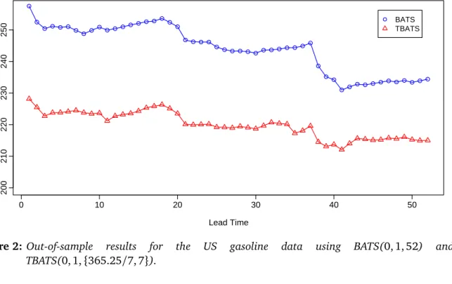
The BATS model was considered next, withm1 =52, and, following the above procedure, it was

discovered that the BATS(0, 1, 52) model withω=φ=1 minimized the AIC. Figure2shows the out-of-sample RMSEs obtained for the two models, and it can be seen that the trigonometric model clearly performs better for all lead times.

This result can be explained by some of the advantages the trigonometric representation has over the traditional seasonal representation. First, the BATS model cannot handle the non-integer frequency, and hence it had to be rounded off to the nearest integer. Second, the BATS model may be over-parameterized, as 52 initial seasonal values have to be estimated for the model. Third, these initial values cannot be optimized along with the smoothing parameters, due to the high dimensionality of the optimization space. These problems are overcome in the trigonometric formulation, which allows for non-integer frequencies and requires fewer initial values to be estimated for the initial seasonal component, hence allowing them to be optimized.

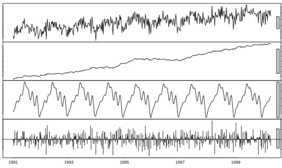
Decomposition of the Gasoline time series obtained using the fitted TBATS model is shown in Figure3. The vertical bars at the right side of each plot are of equal heights but plotted on different scales; thus providing a comparison of the size of each component. The trigonometric formulation in TBATS models allows for more randomness to be eliminated from the seasonal component, yet allowing for those influential bumps to be revealed.

0 10 20 30 40 50 200 210 220 230 240 250 Lead Time RMSE ● ● ● ● ● ● ● ●● ●_{● ●} ● ●● ● ● ● ● ● ● ● ● ● ● ● ● ● ● ● ● ● ●● ● ●● ● ● _● ●● ● ● ● ●● ● ● ● ● ● ● _BATS TBATS

Figure 2: Out-of-sample results for the US gasoline data using BATS(0, 1, 52) and

6500 8000 data 7200 7800 8400 trend −400 0 400 annual −500 0 500 remainder Weeks 1991 1993 1995 1997 1999

Figure 3:Trigonometric decomposition of the US gasoline data.

7.2 Application to call center data

The call center data shown in Figure1(a) consist of 10,140 observations, that is 12 weeks of data starting from 3 March 2003 (Weinberg et al. 2007). They contain a daily seasonal pattern with frequency 169 and a weekly seasonal pattern with frequency 169_∗5=845. The fitting sample consists of 7,605 observations (9 weeks). The trend appears to be close to zero, and hence the growth rate bt was omitted from the models.

The model selection procedure led to the model TBATS(3, 1,_{169, 29_},_{845, 15_}) withω=φ=1 andβ=b₀=0. The BATS model, withm₁=169 andm₂=845, was then considered. The model selection procedure led to the BATS(3, 0, 169, 845) model withω=0.317,φ=1 andβ=b0=0

was chosen. (Other BATS models withω=1 were also tried, but their forecasting performance was worse.)

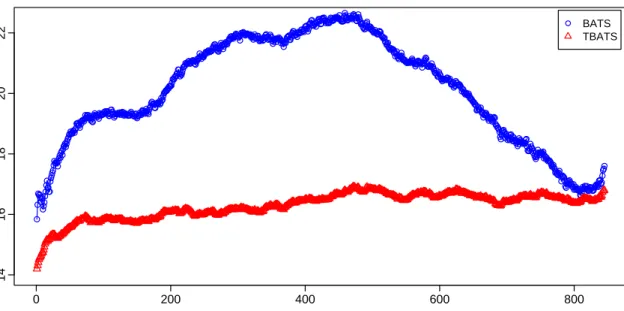
Figure4compares the post-sample forecasting accuracies of the selected BATS and TBATS models, and it can be seen that the TBATS model, which requires the estimation of 102 values, provides much greater forecasting accuracy than the BATS model, which requires the estimation of 1025 values, for all forecast horizons.

0 200 400 600 800 14 16 18 20 22 Lead Time RMSE ● ● ●●●_● ●●● ●●● ●● ●●_●●_●●● ●●● ●● ●●●●●_●●●●● ●●_●●●●●●●● ●●●●●●●●●●●●● ● ●●●●●●●●●●● ● ●_●●●●●●●_●●_●●●●●●●●●●_●●●●●●●●●●●●●●_● ●●●●●●●●_●●●●●●●●●●●●●●_●●●●●●●●●●●●●●●●●●●_● ●●●●●●●●●●●●●●●●●●●● ● ●●●●●_● ●●●●●●●●● ● ●●●●● ● ●●●●●●●●●●●●● ●●●●●●●●●●●●● ● ●●●●●●●●●●●●●●●●_●●●●●●●●●●_●●●●●●●●●●●●●●●●●●●●●●●●●●●●●●●●_●●●●●●●●●●●●● ●●●●●●●●●●●●_●●●●●●●●●●●●●●●●●_●●●_●●●●●●●●●_●●●●●●●●●●●●●●●●●●●_● ●●●●●●●●●●●●●●●_● ●●●● ● ●●●●_● ● ●●●●●●●●●●●●●●●● ●●●●●●●●●●●●●● ● ● ●●●●●_●●●●●●●_●●●●●●●●_●●●●●●●●●●●●●●●●●●●●●●●●●●●● ●●●●●●●●●●●●●●●●●●●●●●●●●●●_● ●●●●●●●●●●●_●●●●●●●●●●●●●●●_●● ●●●●_●● ●●●_● ● ●●●●●●_●● ●●●●●●●●●●●_●●●● ●●●●●●●●●●●●●●●●●●●●●●●●●_●●●●●●● ●●●●●●●●●●_● ●●●●●●●●●●_● ●●●●●●●●●●●●●●_●●●● ●●●●●●●●●●●●_●●●_●● ●●●●●●●_●●● ● ●●●●●● ●●●●●●●●●● ●●●●●●●●●●●●●●●●●● ●●●●●●_● ●●● ●●●● ● ●●●_●●●●●●●●●●●●●_●●_●●●●●●●●●●●●●●_● ●●●●●●●● ●●_● ●●●● ● ●_●●●●●●●_●●●●●●●●●●●●●●●●●_●●●●●●●●● ●●●●●● ●●●●●●●●●●●●●●●●_●●●●●●_●●●●●●●●●●●●●●●●●●●●●●●●●●●● ● ●●_●●● ●●● ● _BATS TBATS

Figure 4: Out-of-sample results for the call center data using BATS(3, 0, 169, 845) and

TBATS(3, 1,_{169, 29_},_{845, 15_})

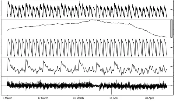
The decomposition obtained from TBATS is shown in Figure5, which clearly exhibits strong daily and weekly seasonal components. The weekly seasonal pattern seems to be evolving rapidly with time while the daily seasonal pattern stays relatively more constant. As is seen from the time series plot itself, the trend component is very small in magnitude compared to the seasonal components.

7.3 Application to the Turkey electricity demand data

The Turkey electricity demand data shown in Figure1(c) have a number of important features that should be reflected in the model structure. Three seasonal components with frequencies m1=7, m2=354.37 andm3=365.25 exist in the series. The sharp drops seen in the seasonal component

with period 354.37 are due to the Seker and Kurban religious holidays, which follow the Hijri calendar, while those seen in the seasonal component with frequency 365.25 are due to national holidays which follow the Gregorian calendar.

In this study, the data, which cover a period of 9 years, are split into two parts: a fitting sample of

n=2191 observations (6 years) and a post-sample period of p=1096 observations (3 years). The order selection procedure was followed and the TBATS(3, 2,_{7, 3_},_{354.37, 23_},_{365.25, 3_}) model withω=0.00165 andφ=1 was selected.

None of the existing exponential smoothing models can handle this time series; however, the BATS model was applied with the frequencies rounded off to the nearest integer (i.e., m1 =7,m2 =

100 300 data 194.5 195.5 trend −100 0 100 daily −40 0 40 weekly −100 0 100 remainder 5 minute intervals

3 March 17 March 31 March 14 April 28 April

Figure 5:Trigonometric decomposition of the call center data.

354,m3 =365), which is expected to affect the accuracy of the forecasts. In addition, this model

requires the estimation of 354+365+7=726 values for the seasonal component alone.

Figure6shows the exceptional post-sample forecasting performance of the TBATS model compared to the BATS model.

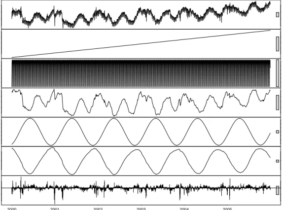
The decomposition of the series obtained by using the chosen TBATS model, is shown in Figure7. The first panel shows the transformed observations and the second shows the trend component. The third panel shows the weekly seasonal component which does not seem to have much variation with time. The fourth panel shows the overall annual component, which is composed of a seasonal component based on the Hijri calendar with frequency 354.37 and a seasonal component based on the Gregorian calendar with frequency 365.25, which are shown separately in the fifth and the sixth panels respectively.

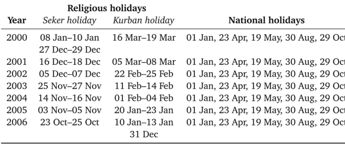
The rather wiggly seasonal components has probably occurred due to the use of a large number of harmonics in each seasonal component. This is necessary to capture the sharp drops seen in the time series plot. If we assume that the stochastic seasonal component is augmented by deterministic holiday effects, we can reduce the number of harmonics required by using dummy variables in handling those sharp drops which occur due to holidays. Table 1gives the dates of the holidays

0 100 200 300 500 1000 1500 2000 2500 Lead Time RMSE ● ● ● ● ● ●● ●●●●●● ●●● ●●●●●●●●●●●●●● ●●●●●● ●●●● ●●●●●●●●● ●●●●●●●●●●●●●●●●_● ●_● ●●● ●● ●●● ●●●●●●●●●●●●●●●●●●●●●●●●●●●●●●●●●●●●●●●●●●●_● ●●●●●●●●●●●●_● ●●●●●●●●●●●●●●●●●●●●●●●●●●●●●●●●●●●●●●●●●●●●●●●●●●●●●●●●●●●●●●●●●●●●●●●●●●●●●● ●●●●●●●●●● ●●●●●●●●●●●●●●●●●●●●●●●● ●●●●●●●●●●●●●●●●●●●●●●●●●●●●●●●●●●●●_● ●_● ●●●● ●● ●●●●●●●●●●●●●●●●●●●●●●●●●●●●●●●●●●●●●_● ●●●●●●●_● ●●●_● ●_● ●●●●●_● ● ● ● ● ● ●●● ● ● ●● ●●●_● ● ● _BATS TBATS

Figure 6: Out-of-sample results for the Turkey electricity demand data using BATS(0, 0, 7, 354, 365)

and TBATS(3, 2,_{7, 3_},_{354.37, 23_},_{365.25, 3_}) 9.0 9.6 10.2 data 9.74 9.80 trend −0.10 −0.02 weekly −0.4 −0.1 0.2 annual −0.3 0.0 Hijri −0.3 0.0 0.3 Gregorian −0.3 0.0 0.2 remainder Days 2000 2001 2002 2003 2004 2005

celebrate the end of the fast of Ramadan. Kurban is a four-day festival when sacrificial sheep are slaughtered and their meat distributed to the poor. In addition, there are national holidays which follow the Gregorian calendar as shown in the table. Using a trend component, a seasonal component and holiday dummy variables, regression was performed on the transformed y_t(ω)values. The term P3_i=1Pki j=1a (i) j cos(λ (i) j t) +b (i) j sin(λ (i)

j t) was used in capturing the multiple seasonality

withk1=3,k2 =k3=1. The estimated holiday effect was then removed from the series and the

remainder was decomposed using TBATS to achieve the decomposition shown in Figure8.

Religious holidays

Year Seker holiday Kurban holiday National holidays

2000 08 Jan–10 Jan 16 Mar–19 Mar 01 Jan, 23 Apr, 19 May, 30 Aug, 29 Oct 27 Dec–29 Dec

2001 16 Dec–18 Dec 05 Mar–08 Mar 01 Jan, 23 Apr, 19 May, 30 Aug, 29 Oct 2002 05 Dec–07 Dec 22 Feb–25 Feb 01 Jan, 23 Apr, 19 May, 30 Aug, 29 Oct 2003 25 Nov–27 Nov 11 Feb–14 Feb 01 Jan, 23 Apr, 19 May, 30 Aug, 29 Oct 2004 14 Nov–16 Nov 01 Feb–04 Feb 01 Jan, 23 Apr, 19 May, 30 Aug, 29 Oct 2005 03 Nov–05 Nov 20 Jan–23 Jan 01 Jan, 23 Apr, 19 May, 30 Aug, 29 Oct 2006 23 Oct–25 Oct 10 Jan–13 Jan 01 Jan, 23 Apr, 19 May, 30 Aug, 29 Oct

31 Dec

Table 1:The dates of Turkish holidays between 1 January 2000 to 31 December 2006.

The fourth panel shows the overall annual component, which comprises the Hijri seasonal effect (fifth panel) and the Gregorian seasonal effect (sixth panel). It is seen that this now provides a much smoother seasonal decomposition and only one harmonic is required for each seasonal component (i.e.,k2=k3=1) in capturing seasonal calendar effects. This analysis demonstrates the capability of

our trigonometric decomposition in extracting those seasonal components which are otherwise not apparent in graphical displays. Existing decomposition techniques are unable to handle such complex seasonalities.

In forecasting complex seasonal time series with such deterministic effects, both BATS and TBATS models may be extended to accommodate regressor variables, allowing additional information to be included in the models.

9.4 9.8 data 9.65 9.80 trend −0.10 −0.02 weekly −0.10 0.05 annual −0.6 0.0 0.6 Hijri −0.5 0.5 Gregorian −0.2 0.0 remainder Days 2000 2001 2002 2003 2004 2005

Figure 8: Trigonometric decomposition of the regressed Turkey electricity demand data.

8

Concluding remarks

A new state space modeling framework, based on the innovations approach, is developed for forecasting time series with complex seasonal patterns which cannot be forecast using any current forecasting approaches. The new approach not only offers an alternative to both linear and non-linear traditional exponential smoothing models, but also has many advantages and provides additional options, some of which are not seen in any of the existing forecasting approaches. The new approach is also capable of decomposing and forecasting time series with multiple seasonality, high frequency seasonality, non-integer seasonality and dual calendar effects.

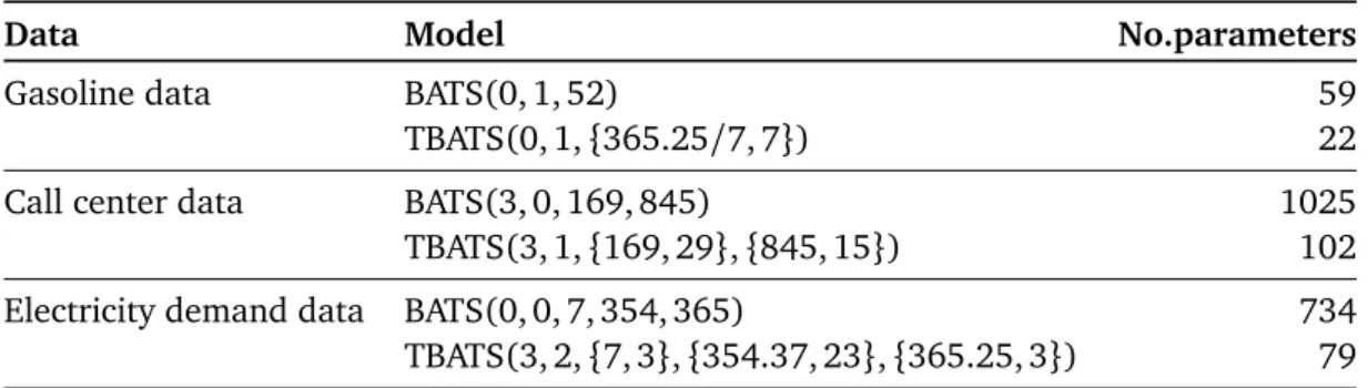
The superiority of the new modeling framework in handling such seasonal patterns is illustrated in three empirical studies, where it is shown to greatly improve the out-of-sample forecasting accuracy. It is also shown that our trigonometric approach offers an elegant way of decomposing complex seasonal time series, which cannot be decomposed using any of the existing methods. Table 2

than traditional seasonal exponential smoothing models in all three applications. Moreover, these models also overcome the weaknesses of the existing exponential smoothing models, such as the instability of non-linear models and correlated errors.

Table 2: Number of estimated parameters for each model in each application.

Data Model No.parameters

Gasoline data BATS(0, 1, 52) 59

TBATS(0, 1,{365.25/7, 7}) 22 Call center data BATS(3, 0, 169, 845) 1025 TBATS(3, 1,{169, 29},{845, 15}) 102 Electricity demand data BATS(0, 0, 7, 354, 365) 734 TBATS(3, 2,{7, 3},{354.37, 23},{365.25, 3}) 79

Acknowledgement

We thank Ralph Snyder and Peter Toscas for helpful comments that improved this paper. We are also grateful to Derek K. Baker and Merih Aydinalp Koksal for providing the Turkish electricity data.

Appendix A

Equation (2) can be written in the following form:

s_t= k X j=1 (cosλ_jt, sinλ_jt)0x_j,t (12) x_j,t=xj,t−1+κt, (13)

wherex_j,t= (α_j,t,β_j,t)0andκt= (k₁"_t,k₂"_t)0. We re-parameterize using

x_j,t=A_j,ts_j,t, where sj,t = (sj,t,s∗j,t)0 andAj,t =    cos(λ_jt) ₋sin(λ_jt) sin(λ_jt) cos(λ_jt)  

. Then, substituting this into equation

(13), we obtain A_j,ts_j,t=A_j,t−1s_j,t−1+κt s_j,t=A−_j,1_tA_j,t−1s_j,t−1+A−_j,1_tκt, where A−_j,t1 =    cos(λ_jt) sin(λ_jt) −sin(λ_jt) cos(λ_jt)  

. Using well-known trigonometric identities, A

−1 j,tAj,t−1 =    cos(λ_j) sin(λ_j) −sin(λ_j) cos(λ_j)  

References

Akram, M., Hyndman, R. J. & Ord, J. K. (2009), ‘Exponential smoothing and non-negative data’,

Australian & New Zealand Journal of Statistics51(4), 415–432.

Archibald, B. C. & Koehler, A. B. (2003), ‘Normalization of seasonal factors in Winters’ methods’,

International Journal of Forecasting19, 143–148.

Billah, B., Hyndman, R. J. & Koehler, A. B. (2005), ‘Empirical information criteria for time series forecasting model selection’,Journal of Statistical Computation and Simulation75, 831–840. Box, G. E. P. & Cox, D. R. (1964), ‘An analysis of transformations’, Journal of the Royal Statistical

Society, Series B26(2), 211–252.

Burnham, K. P. & Anderson, D. R. (2002), Model selection and multimodel inference: a practical information-theoretic approach, 2nd edn, Springer-Verlag.

Chatfield, C. (1978), ‘The Holt-Winters forecasting procedures’,Applied Statistics27, 264–279. Durbin, J. & Koopman, S. (2001),Time series analysis by state space methods, Oxford University Press. Gardner, Jr, E. S. (1985), ‘Exponential smoothing: The state of the art’,Journal of Forecasting4, 1–28. Gilchrist, W. (1976),Statistical Forecasting, Wiley: Chichester.

Gould, P. G., Koehler, A. B., Ord, J. K., Snyder, R. D., Hyndman, R. J. & Vahid-Araghi, F. (2008), ‘Forecasting time series with multiple seasonal patterns’,European Journal of Operational Research

191(1), 207–222.

Hannon, E. J., Terrel, R. & Tuckwell, N. (1970), ‘The seasonal adjustment of economic time series’,

International Economic Review11, 24–52.

Harvey, A. (1989),Forecasting structural time series models and the Kalman filter, Cambridge University Press.

Harvey, A. & Koopman, S. J. (1993), ‘Forecasting hourly electricity demand using time-varying splines.’,Journal of the American Statistical Association88, 1228˝U1236.

Harvey, A., Koopman, S. J. & Riani, M. (1997), ‘The modeling and seasonal adjustment of weekly observations’,Journal of Business and Economic Statistics15, 354–368.

Hyndman, R. J., Akram, M. & Archibald, B. C. (2007), ‘The admissible parameter space for exponential smoothing models’,Annals of the Institute of Statistical Mathematics60, 407–426.

Hyndman, R. J., Koehler, A. B., Ord, J. K. & Snyder, R. D. (2005), ‘Prediction intervals for exponential smoothing using two new classes of state space models’,Journal of Forecasting24, 17–37. Hyndman, R. J., Koehler, A. B., Ord, J. K. & Snyder, R. D. (2008), Forecasting with exponential

smoothing: the state space approach, Springer-Verlag, Berlin.

URL:www.exponentialsmoothing.net

Hyndman, R. J., Koehler, A. B., Snyder, R. D. & Grose, S. (2002), ‘A state space framework for automatic forecasting using exponential smoothing methods’,International Journal of Forecasting

18(3), 439–454.

Hyndman, R. & Khandakar, Y. (2008), ‘Automatic time series forecasting: The forecast package for R’,

Journal of Statistical Software26(3).

Koopman, S. J. & Lee, K. M. (2005), ‘Measuring asymmetric stochastic cycle components in U.S. macroeconomic time series’, (05-081/4).

URL:http://ideas.repec.org/p/dgr/uvatin/20050081.html

Lin, J. & Liu, T. (2002), ‘Modeling lunar calendar holiday effects in Taiwan’,Taiwan Economic Forecast and Policy33(1), 1–37.

Makridakis, S., Anderson, A., Carbone, R., Fildes, R., Hibon, M., Lewandowski, R., Newton, J., Parzen, E. & Winkler, R. (1982), ‘The accuracy of extrapolation (time series) methods: results of a forecasting competition’,International Journal of Forecasting1, 111–153.

Makridakis, S. & Hibon, M. (2000), ‘The M3-competition: Results, conclusions and implications’,

International Journal of Forecasting16, 451–476.

Ord, J. K., Koehler, A. B. & Snyder, R. D. (1997), ‘Estimation and prediction for a class of dynamic nonlinear statistical models’,Journal of the American Statistical Association92, 1621– 1629. Ord, J. K., Snyder, R. D., Koehler, A. B., Hyndman, R. J. & Leeds, M. (2005), Time series forecasting:

the case for the single source of error state space approach, Working paper 7/05, Department of Econometrics & Business Statistics, Monash University.

compo-Pole, A., West, M. & Harrison, J. (1994),Applied Bayesian forecasting and time series analysis, Chapman & Hall/CRC.

Proietti, T. (2000), ‘Comparing seasonal components for structual time series models’,International Journal of Forecasting247-260, 16.

Reid, D. J. (1975), A review of short-term projection techniques. Practical aspects of forecasting, Operational Research Society: London.

Riazuddin, R. & Khan, M. (2005), ‘Detection and forecasting of Islamic calendar effects in time series data’,State Bank of Pakistan Research Bulletin1(1), 25–34.

Snyder, R., Koehler, A. & Ord, J. (2002), ‘Forecasting for inventory control with exponential smooth-ing’,International Journal of Forecasting18(1), 5–18.

Taylor, J. (2008), ‘An evaluation of methods for very short-term load forecasting using minute-by-minute British data’,International Journal of Forecasting24(4), 645–658.

Taylor, J. (2009), ‘Triple seasonal methods for short-term electricity demand forecasting’,European Journal of Operational Research.

Taylor, J. W. (2003a), ‘Exponential smoothing with a damped multiplicative trend’,International Journal of Forecasting19, 715–725.

Taylor, J. W. (2003b), ‘Short-term electricity demand forecasting using double seasonal exponential smoothing’,Journal of the Operational Research Society54, 799–805.

Taylor, J. W. & Snyder, R. D. (2009), ‘Forecasting intraday time series with multiple seasonal cycles using parsimonious seasonal exponential smoothing’, (9/09).

URL:http://ideas.repec.org/p/msh/ebswps/2009-9.html

Weinberg, J., Brown, L. & Stroud, J. (2007), ‘Bayesian forecasting of an inhomogeneous Poisson process with applications to call center data’, Journal of the American Statistical Association

102(480), 1185–1198.

West, M. & Harrison, J. (1997),Bayesian forecasting and dynamic models, 2nd edn, Springer-Verlag, New York.