Crosswalk Identification
for Decision Making
Paraskevi Christodoulou
SID: 3308170006SCHOOL OF SCIENCE & TECHNOLOGY
A thesis submitted for the degree of
Master of Science (MSc) in Data Science
DECEMBER 2018
Crosswalk Identification
for Decision Making
Paraskevi Christodoulou
SID: 3308170006Supervisor: Rigas Kotsakis
SCHOOL OF SCIENCE & TECHNOLOGY
A thesis submitted for the degree of
Master of Science (MSc) in Data Science
DECEMBER 2018
Abstract
This dissertation is a part of the MSc in Data Science at the International Hellenic University. The main topic of this research was the identification of crosswalks through images in order to use the results for further decision making. The idea has emerged from the ever-evolving car industry, in which more and more manufacturers are leaning towards the autonomous driving. Driverless vehicles were just a dream a few decades ago, but now they are closer to become reality than ever before. There are already autonomous systems, like Cruise Control and Emergency Braking system, which give drivers the opportunity to already enjoy some privileges of driverless driving. Nevertheless, the target is to reach an autonomous level such that no human intervention will be necessary. For that reason, crosswalk identification is also a crucial aspect in autonomous driving since crosswalks are places where the possibility to meet an obstacle is really high. Thus, a system that identifies them should be implemented in order to make decisions itself such as whether to slow down or even stop the vehicle without the drivers’ help. Briefly, this dissertation contains the process of knowledge extraction from images in Matlab as well as the classification procedure in Weka, in which different classifiers have been trained and tested regarding the presence of a crosswalk. In addition, the dataset that was used in the experiments was a primary material which contained images from roads across Thessaloniki, the second largest city of Greece.
Acknowledgement
I would like to acknowledge my thesis supervisor, Prof. Riga Kotsaki, for his consulting services, my brother, Nickolao Christodoulou, for his contribution as the photographer of the dataset images and the two colleagues of mine, Charalampia Komopoulou and Aikaterini Mantela, for their participation into the annotation process of the images. At last, I would like to acknowledge Christo Kasketi for his contribution in the final English language editing of this dissertation.
CONTENTS
Abstract ... 3 1. INTRODUCTION ... 5 2. RELATED WORK ... 10 3. DATASET ... 21 3.1. Crosswalk characteristics ... 21 3.2. Dataset description ... 22 4. TOPIC DESCRIPTION ... 265. FEATURE EXTRACTION PROCESS ... 28
5.1. Contrast ... 29 5.2. Homogeneity ... 30 5.3. Correlation ... 30 5.4. Energy ... 30 5.5. Entropy ... 31 5.6. Statistical Measures ... 31 5.7. Edges ... 32 5.8. Lines ... 33 5.9. Rectangles ... 33
5.10. Number of white pixels ... 34
6. CLASSIFICATION & EXPERIMENTAL RESULTS ... 35
6.1. Attributes’ Evaluation ... 35 6.2. Classifiers’ Description ... 36 6.2.1. Decision Trees ... 36 6.2.2. Statistical Regression ... 37 6.2.3. Bayesian classifiers ... 39 6.3. Evaluation metrics ... 39 6.4. Experimental results ... 40
6.4.1. 10-fold Cross Validation ... 42
6.4.2. 5-fold Cross Validation ... 43
6.4.3. 2-fold Cross Validation ... 45
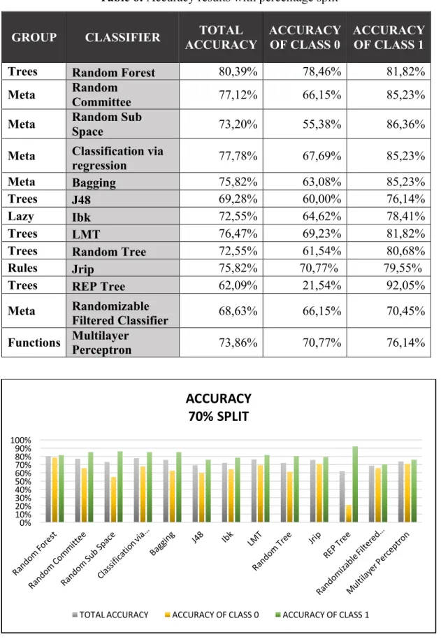
6.4.4. Percentage split ... 46
7. CONCLUSION – DISCUSSION ... 49
8. FUTURE WORK ... 50
APPENDICES ... 51
A. Granting Rights ... 51
B. Matlab code sample ... 51
C. “.arff” file sample ... 53
1.
INTRODUCTION
In the past, it was only in people’s dream that in the near future there will be self-driving cars that will “feel” their environment and react accordingly to each situation with a little or even without the help of humans (Thrun & Sebastian, 2010). Autonomous vehicles have different kinds of sensors like radars, GPS, LIDAR, computer vision and odometer, which are responsible for giving information so that the vehicle could navigate itself and even more recognize potential obstacles on the road.
Driverless cars like that have a lot of benefits in different fields. Such benefits involve cost and traffic collision reduction, traffic flow and safety increase, a better and improved mobility for children, elderly and disabled people as well as more restful traveling conditions for travelers (Azizi, Pushkin, Gueraiche, & Hamid, n.d.).
However, there is a giant gap between fully manual and fully automated driving. Thus, SAE International (Society of Automotive Engineers) published a 6-level classification system in 2014, describing the transition from the fully manual to the fully automated driving systems, as shown in the picture below (image 1) (SAE, 2014).
Image 1: SAE International autonomous level (SAE, 2014)
In more detail, level 0 is the fully manual system where drivers control the entire process. Level 1 is when the driver and the system have both the control. For example,
in some cases like Adaptive Cruise Control, the system is responsible for the maintenance of the speed while the driver controls the steering and in some other cases like Parking Assistance where the process is inverted, the system controls steering and the speed is manually defined. However, in any case, the driver should be able to take the full control in any time needed. In Level 2, steering, braking and accelerating are automated by the system and the driver must only monitor the driving in order to interfere in any time. Likewise, in level 3, the whole process is automated again by the system, but now the driver could safely do also other things and not pay attention to the driving at all. However, there is also the need here for the driver to interfere, but only at the time when the vehicle is asking to do it. Moving forward to Level 4, there is no need for the driver to pay attention to any phase of driving under specific circumstances. Apart from these cases, the vehicle should be able to park the car if the driver never interacts at all. Last but not least, level 5 is the fully automated stage, where the system never demands a human intervention (SAE, 2014).
Autonomous driving experiments took place in the 1920s (Sentinel, 1920) and the first trials implemented in the 1950s. In 1977, a Mechanical Engineering Laboratory developed a truly automated vehicle, which could be able to identify the white street markets from two cameras that were installed on the vehicle. It could also reach speeds of up to 30km/h with the help of an elevated rail (Thrun & Sebastian, 2010). Since then, a lot of autonomous prototype cars appeared in the early 2000s, the first self-parking systems were introduced and made the autonomous vehicles dream more realistic than ever. Specifically, Toyota’s Japanese Prius hybrid vehicle and Lexus LS sedan introduced an automatic parallel parking assistance in 2003. A few years later, in 2009, Ford offered the Active Park Assist and in 2010, BMW released its own automated parallel parking assistance. Also, in 2009, Google started developing its own self-driving car secretly, which is now called Waymo and had covered about 482.803 kilometers with only computer control and without any accident occurred. Furthermore, in 2014, Google introduced a driverless car with the absence of steering wheel, gas and brake pedal, which by the end of 2017 had done more than 3 million kilometers. In addition, the 2014 Mercedes S-Class included semi-autonomous features like the ability of the car to stay within road lines or avoid accidents as well as self-steering (Dormehl & Edelstein, 2018).
In fact, by 2013, almost all car companies such as General Motors, Ford, Mercedes Benz, BMW, and others were working on several self-driving car
technologies. Specifically, Nissan claims that it will present several autonomous driverless cars by 2020, while Audi insists that the A8 luxury sedan will be the first car with a Level 3 autonomy system according to SAE. The specific model will include the A8’s Traffic Jam Pilot which will allow the car to navigate itself without any driver intervention. This automated system will work only under certain circumstances, which will allow speeds up to 60km/h in traffic and work perfectly with clearly-hatched entrance and exit lanes in highways (Dormehl & Edelstein, 2018).
According to the autonomous car history above, it is obvious that the future consists of smart and driverless vehicles, which will give the potentials to improve the quality of human lives. At first, according to experts, traffic jams would be eliminated, since many times traffic collisions are caused by human mistakes, like distracted or nervous drivers (Cowen, 2011; Whitwam, 2014; Zhang, 2014). Also, travelers could spend those driving hours by doing something else more beneficial for them or spend this time working. In addition, it would be a great opportunity for mobility enhancement for children, elderly or disabled people. In any case, there will be more prosperity in human lives (Cowen, 2011; Zhang, 2014).
Moreover, one article mentions that in highways, drivers usually keep a safe distance of about 40m away from the leading car, which increases the highway capacity and results in traffic collisions. Hence, authors claim that using autonomous and connected vehicles, the distance between one car and another could be only 6m and traveling could be safe even at 120km/h. Also, having safer driving conditions result in reduced vehicle insurance costs and in higher fuel economy since autonomous cars would be able to break or accelerate more efficiently (Ackerman, 2012).
Nowadays, vehicles have already automated features regarding emergency braking, cruise control for speed management and automated systems that keep the vehicle inside road lanes. Specifically, cruise control is a system, which gives the opportunity to drivers to define a specific speed level, leave the gas pedal and let the system maintain that speed. In this case, drivers control only the steering wheel and the brake pedal and they are able to take the full control of the vehicle back in any time needed. Moreover, emergency braking system is an autonomous feature that automatically activates the brakes in case of a collision. At first, it warns the driver in order to give him the time to interfere, and if he doesn’t respond in time, the system brakes the car by its own. Most car companies are using a combination of tools such as cameras and sensors in order to implement this feature. Sensors are able to detect the
distance between the car and the obstacle in front of it and cameras, which are placed closed to the rear-view mirror, are capable of identifying the nature of the objects. Hence, in case of a collision, the system warns the driver with an audio and visual signal. If the driver doesn’t respond immediately, the system pushes the brakes and gives some assistance to the driver in order to fill the gap of not responding on time. At last, if the driver still doesn’t respond, the system moves into the full stop mode.These systems are made for helping drivers to avoid potential accidents and in cases when the crash is unavoidable to reduce the damage by reducing at least the speed of the car (Nowak, 2018).
Nevertheless, despite all the benefits that driverless cars could bring, there are also some challenges regarding automated processes referred to privacy, moral and ethical issues. Also, fatal incidents have been already recorded around the world related to autonomous vehicles and many question marks are raised in the air. Hence, a lot of research and experiments should be implemented in order to produce more accurate and specialized results.
Additionally, in the same context of autonomous driving is the identification of a crosswalk. Crosswalks are placed in order to help pedestrians cross the road. Even though it is a road mark, the probability of meeting obstacles like pedestrians is really high. Thus, the development of automated systems that can automatically identify crosswalks and make decisions is mandatory in autonomous and driverless driving. However, in order to jump into the implementation of automated systems like that, which will make decisions regarding stopping or slowing up the car, it is firstly necessary to recognize and locate the crosswalks. Many types of research have been done so far and they will be presented in section 2. In addition, this research is also an effort of correctly identifying crosswalks from images in order the results to be used in a future car tool, which will contribute in automating the process of driving with more accurate and safer results. The experiments were implemented in Matlab (The MathWorks, 2017), where feature extraction was made from images that have been manually captured and then the results were used for classification using the Weka platform in order to calculate the accuracy of different models (Hall et al., 2009).
Specifically, this research contains the following. Section 1 is a brief introduction in autonomous driving and the related topic of this paper, which is the identification of a crosswalk through images. All the related work from other researchers, who have done a similar research in crosswalks - identification can be
found in section 2. Moving forward to section 3, the used dataset is presented and in section 4 there is a description of the whole process from the conception of the idea to its realization through the process and all the experiments that have been carried out. In addition, section 5 and 6 include the feature extraction in Matlab and the classification process in Weka respectively, while section 7 summarizes the entire research. Finally, section 8 is a discussion regarding suggestions for future analysis and the implementation of an autonomous car tool.
2.
RELATED WORK
In the literature, several approaches to the crosswalk detection problem were found and a large number of different kinds of proposed algorithms and systems were retrieved. The main scope for the majority of the articles focuses on detecting a crosswalk for pedestrian safety reasons, either for helping visually impaired people or for autonomous driving systems.
In the case of people with visual disabilities, an application on a cell phone was presented in an article. The city intersections are too dangerous for visually impaired or blind people. Thus, to help those people in situations like that, authors present the “Crosswatch system”, which uses only computer vision from a camera cell phone in order to address the orientation and the location of a crosswalk. The system was installed on a Nokia N95 camera phone and runs in real time by automatically taking a few pictures per second, analyzes them and produces a sound when it identifies a crosswalk. The algorithm was implemented in two parts. The first one was the feature extraction and especially the extraction of straight lines from the images using some edge filtering since crosswalks consist of typical white colored lines. After that, a factor graph model was used in order to classify them into crosswalk and background classes. In addition, the algorithm was implemented in Matlab with 25 images as a train set and 90 images as a test set, where only 30 of them included a crosswalk. The results have shown that the true positive rate of the algorithm was 72% and the false positive one was 0.5%. Also, the model is able to locate the general borders of a crosswalk and provides the user with an audio notation, like “the crosswalk is at 12 o’clock”, in order to direct properly and safely blind people in the direction of the crosswalk (Ivanchenko, Coughlan, & Shen, 2008).
From the same perspective, in another article a wearable system that captures images in RGB-D form is presented. The colored images were 2500 and after filtering, a Convolutional Neural Network was trained and evaluated. The accuracy level was 88.97% and after some head adjustments, it became 91.59% (Poggi, Nanni, & Mattoccia, 2015). RGB-D images were also used in order to detect stairs, crosswalks and traffic lights. For the crosswalk and the stair detection part, authors proceeded in image processing by extracting the depth feature and used a Support Vector Machine classifier in order to discriminate them. The dataset included 228 images, from which
only 30 of them have a crosswalk, and consequently their algorithm has an accuracy of 78.90% (Wang, Pan, Zhang, & Tian, 2014).
Moreover, authors in another article proposed a crosswalk classification system, which was implemented based on deep learning. Specifically, the system takes advantage of platforms, such as Google Street View, in order to train a Convolutional Neural Network (CNN) to automatically classify an image in real-time based on the existence of a zebra crossing in a developing country like Brazil. Also, the paper includes a comparison study between two models. One model uses completely automatic image annotation, in contrast to the other, which uses a partially manually one. Furthermore, the total system is presented in two parts. The first one is the automatic data retrieval, where the data was downloaded, processed and annotated automatically, and the second one is the Convolution Neural Network training phase, where the CNN model is trained and then used to classify new unseen before images (Berriel, Rossi, de Souza, & Oliveira-Santos, 2017).
According to the same paper, the gain and the annotation of a large dataset is very crucial and important for the CNN part. The images can be annotated fully automatically or manually by users, who can change part of the dataset in order to correct potential mistakes and increase the final accuracy. In the case of automatically acquisition, the only thing that users should do is the outline of the appropriate regions, which are in a rectangular form. The user can select one or more areas of interest, and for each area the system looks for crosswalk locations according to OpenStreetView. All regions must be no bigger than ¼ degrees, so anything above that threshold is automatically divided into sub-areas. Then, another separation is put into effect in order to end up having sub-areas with more than 50 and less than 2000 crosswalks. Following the procedure above, all crosswalk locations have been identified. However, it is also very important to identify locations very close to the crosswalk places, which can become feasible using Google Maps Directions API.
After that, the annotation part took place. First, there was the automated process, where images that include a crosswalk located within a specific range of view were described as a positive sample. In any other case, the sample was characterized as negative. Also, there was the manual annotation process where users made the decision whether an image includes a crosswalk or not having two specific things in mind: (a) all crosswalks should capture a satisfying part of the image and (b) all crosswalks should be from the vehicle point of view.
As mentioned before, authors trained a CNN, which contains 16 layers, 13 convolutional and 3 fully connected layers. However, the last layer was transformed with only 2 neurons, one for each category, positive (crosswalk inclusion) and negative (crosswalk absence) sample. Also, for the training phase, all images were downsized to 256 x 256 pixels.
Moreover, the proposed system used three different datasets, Google Street View, IARA and GOPRO dataset. The Google Street View dataset was retrieved and annotated automatically and all images were from Brazilian roads. However, there were some challenges in this dataset, such as in some cases the crosswalk paint was fading away, there were shadows from different objects like vehicles, trees, and pedestrians or there were different colored crosswalks. The second dataset was the IARA dataset, which was a collection of images taken by an autonomous car, the Intelligent Autonomous Robotic Automobile (IARA). It is an autonomous car that was developed in the High-Performance Computing Lab of a university in Brazil. The vehicle contains many sensors, but only a camera placed on top of the car and facing forward was used to collect the dataset images. The images were taken during day and night in a weekday and in total, there were 12.441 images from 4 different sequences in Vitoria. At last, the GOPRO dataset consists of 11.070 images from different city roads and highways.
For the system evaluation, accuracy and F1 score were mainly used. However, the authors proposed one more metric, the instance accuracy, which uses crosswalks as instances. In more details, this metric will be positive only if the system classifies correct at least the half of a sequence, which means that if a crosswalk is included in 20 images in a row, the system should classify correctly at least 10 of these images. At last, for the statistical analysis, the t-test has been used as well. The experiments on the fully automatic annotated dataset gave an accuracy of 94.12% and 89% of the F1 score. In contrast to that, the partially automatic dataset gave 96.3% and 92.78%, respectively. So, it is observed that both accuracy and F1 level have a slight improvement as expected.
After the evaluation, authors also investigated why some images were annotated incorrectly and they end up with the following observations. When an image was manually annotated as positive, but the system classifies it as a negative one, the errors have been occurred because of authentic mistakes, powerful obstructions and not preserved and different kind of crosswalks. On the other side, when the image was manually labeled as negative and the system predicted it as positive, the problems
occurred because crosswalks were too far or were not in the traffic direction and sometimes there were other road signs on the crosswalk (Berriel, Rossi, et al., 2017).
A very similar approach is presented by almost the same authors as in the previous paper in a letter form, where similar steps were taken in order to classify images regarding the presence of a crosswalk from satellite pictures. Briefly, the system consists of two parts, the automatic image retrieval, and labeling and the classification part using deep learning, CNN. First, users choose the areas of interest, which are in a rectangular shape, OpenStreetMap locates crosswalks within those regions and Google Static Maps API downloads those images. Then the labeling is achieved automatically since the crosswalk locations were known and consequently those images were used to train a CNN. In this experiment, there are two main model categories. The first one is the “intra-based” model, where crosswalks belong to the same city, same country etc. and the second one is the “cross-based” model, where the model has been trained with some images and assessed with some others with the same locality (Berriel, Lopes, de Souza, & Oliveira-Santos, 2017).
Three different architectures were evaluated for this experiment, AlexNet, VGG and GoogleNet with 5, 16 and 22 layers, respectively. The results showed that VGG had a better performance than the others since its accuracy level using intra-based model was slightly higher in both city and country landscapes. The intra-based model achieved almost 97% of accuracy in contrast to the cross-based model, which achieved a lower accuracy level in average (Berriel, Lopes, et al., 2017).
One more related approach that uses satellite imagery is the paper that describes the following. The article uses two kinds of images, the high-resolution ones, where road lines, cars, and crosswalks are visible in details and images based on the surface elevation. Authors implemented a circle mask template and a Speeded Up Robust Features (SURF) method so as to identify and evaluate the crosswalk location in a colored aerial picture. The experiment results showed that their method identifies 306 crosswalks in only 739.2 seconds and the accuracy level is 96.5%, which means that the proposed algorithm can run quickly enough and produce a really good accuracy (Herumurti, Uchimura, Koutaki, & Uemura, 2013).
Another system, which uses aerial geospatial images in order to locate crosswalks and improve guidance applications for visually impaired people, is presented in another article. The proposed algorithm, which has been trained automatically with known data, comprised of the Histogram of Oriented Gradients
(HOG) method and the Local Binary Pattern Histograms (LBPH) method. Also, Support Vector Machine (SVM) has been used for the classification part (Koester, Lunt, & Stiefelhagen, 2016).
Firstly, the aerial images were retrieved from different sources like AeroWest and Google Maps and were preprocessed regarding road locations and directions from OpenStreetMap. Following, a combination of HOG and LBPH were extracted and the SVM was used for classification. Furthermore, the resulting classifier was also used for detecting yet uncharted crosswalks on images, which then are needed to be validated by hand. The results presented a high accuracy level of 98,9% in case of the HOG method with 20 x 20 block size and a radial basis function SVM kernel, compared to 92,4% of the same method with 30 x 30 block size and linear SVM kernel. However, the LBP method has a great performance as well with an accuracy of 98,4%, but a really high precision of 99,7% (Koester et al., 2016).
Staying in the same perspective of aerial images, some other authors proposed an algorithm for automatic crosswalk detection from LiDAR mobile data. Taken images were preprocessed at first with several techniques and segmentation and from the 30 images with crosswalks, 25 of them (83.33%) were classified correctly. However, authors investigated the images that are misclassified and the errors occurred due to paint distortion and obstruction from other objects like cars (Riveiro, González-Jorge, Martínez-Sánchez, Díaz-Vilariño, & Arias, 2015).
Traffic light detection is also a crucial aspect to take into consideration since traffic lights and crosswalks exist together. Most of the algorithms use data not only from images but also from GPS (Levinson, Askeland, Dolson, & Thrun, 2011) or camera calibration (Tae-Hyun, In-Hak, & Seong-Ik, 2006). For example, in the first case, authors propose a traffic light detection algorithm using camera calibration rates, pictures from that camera and GPS location data, while in the other article an algorithm, which uses probability graph with all the global positions of traffic lights.
Another approach is presented in another paper, where the main purpose was to introduce an algorithm that identifies crosswalks and traffic lights with as reduced false negative and positive errors as it can. An assumption that those two exist frequently together was also taken. Their algorithm was created to operate in real time with small computational complexity. In addition, authors were focused more on decreasing false negative rather than false positive errors, since the target was to install the specific
algorithm on Autonomous Vehicle System (AVS), where missing a crosswalk is more harmful than a misdetection one (Choi, Ahn, & Kweon, 2013).
For the crosswalk detection, all images were preprocessed following specific steps. At first, the original images were converted to V ones and after that, 1-D mean filters were applied. Then, using the previous filtered pictures, the algorithm produced two binary pictures, which are retrieved by setting a threshold θ between the original V image and the filtered ones. For the first binary picture, if each pixel’s difference was larger than θ, it became 1. However, for the other binary image each pixel assigned to 1 when the difference was smaller than -θ. After that, those images were denoised through corrosion, expansion, and blob-labeling and then these two denoised binary images were converted into one using the OR operation. The final picture indicates the presence and the location of a crosswalk if the result of the filter is larger than a foregone threshold (Choi et al., 2013).
As for the traffic light detection, authors considered an algorithm from another paper (Levinson et al., 2011) and they tried to improve it in order to solve the problem of time since the referred algorithm was too slow and with high computational complexity. Firstly, the original image was converted to HSV (hue, saturation, value) domain image so as to ensure the robustness in brightness changes and then U, which is the probability that each pixel is the traffic light center, was computed as in (Levinson et al., 2011). At next, the G (H, S, V), which is the probability that each pixel looks like a traffic light, was evaluated. G was also calculated describing a rectangular black area, but it was excluded so as to keep computational complexity low. In addition, a Gaussian- filtered template T was computed.
However, probability G was not able to detect a non-circular object. So, the traffic light could only be identified by the combination of a G image and a circle kernel T. Moreover, according to the above, each pixel has too many values as the template size and thus an R image is also taken, which is the combination of images G and C.
As mentioned before, authors made the assumption that crosswalks are placed next to traffic lights. Each algorithm separately gives very frequently false positive errors and small false negative errors. In contrast to that, when the two algorithms are combined into one, false positive errors are significantly lower. So, the combination of the two algorithms can be generalized since it doesn’t miss any target and the false positive level is low.
The proposed algorithm was implemented by using videos from cameras located on a vehicle. The first camera was a zoom one for a faraway view, the second one was a camera placed in front of the car for the front view and the last one was a bent camera facing down the road. For the traffic light detection, the algorithm used the zoom and the front camera and for the crosswalk identification, the tilted camera. Also, the ground truth included pictures with crosswalks and traffic lights together, which were annotated manually by users. The algorithm results showed that true positive (TP) level is bigger than 95%, so the false negative one is less than 5%. It was also observed that the false positive ratio was 0,02% in case of the combined algorithm in contrast to the false positive ratios from individual traffic light and crosswalk algorithms, which was 0,23% and 0,66% respectively (Choi et al., 2013).
In addition, there are papers, in which authors presented a crosswalk classification algorithm based on an aggregation of Hough transform (Se & Brady, 2003), some others using Fourier transform and augmented bipolarity (Sichelschmidt et al., 2010), while some others proposed a crosswalk detection system after implementing all road markings recognition (Foucher, Sebsadji, Tarel, Charbonnier, & Nicolle, 2011).
Due to the numerous pedestrian accidents in Japan and Europe and especially in urban areas where many citizens live, authors indicate that the already proposed systems like LIDAR sensor are not enough to prevent such accidents. Also, it is very important for systems like that to be implemented in a way that they could become commercial at a low cost and be installed in vehicles. For that reason, the paper introduces an ongoing crosswalk identification system with the usage of a monocular camera and a warning system for pedestrians (Sakai et al., 2013).
It has been shown that mortality rates in Europe, Japan and the, US are 17%, 35%, and 12% respectively. Thus, authors emphasize the importance of such advanced systems in order to protect pedestrians and reduce the fatalities rates. In this research, two approaches were implemented. The first one consisted of the combination of a millimeter wave radar and a monocular camera, which retrieve information about moving objects and crosswalk locations. And the second one was a classification algorithm that detects pedestrian appearances, which tends to increase the computational cost in image processing.
However, the same authors have introduced the efficiency of the first approach in order to reduce the high computational cost. Their algorithm is based on the
assumption that all objects that are moving on a crosswalk could be identified as pedestrians. Hence, the pedestrian detection algorithm is not mandatory in the image processing and the main task should be the crosswalk identification in front of the car. The experiments were made using a vehicle, which was reinforced with a monocular camera that identifies lines, traffic signs and other vehicles and a PC computer for data retrieving and processing.
As mentioned before, an assumption that all moving objects were considered as pedestrians is made. Thus, the algorithm of image processing is depended only on the images that the ongoing front camera captures so as to detect the presence of a crosswalk and to provide a warning notification to drivers in order to prevent a potential accident. The first step, that the proposed system is using, is to binarize, detect the edges with Canny’s algorithm and combine those two from the input images. At next, the algorithm classifies the pattern regarding the vertical edge changes into two types. One category is the outer limit where the brightness changes from dark to light and the other one is from bright to light. Then, a measure to detect a crosswalk, called “cross-ratio”, was used and it was calculated given four collinear points by the following formula.
As for the second part, where the pedestrian detection took place, the algorithm followed the next steps. First, the region of interest (ROI) was retrieved regarding the distance of the crosswalk. After that, in order to get the visual flow vectors, the system calculates the visual flow only inside that region. Next, the visual flow vectors which diverge from the crosswalk lines and the distance between those lines and edges is higher than a threshold are categorized as “outliers”. Those outliers that are closer together are merged and classified as moving objects and consequently as pedestrians. After some experiments in Japan, the proposed algorithm had a true positive rate of 90%, which means that in the 90% of the cases the system identifies correctly the presence of a crosswalk (Sakai et al., 2013).
Another paper also describes how the warning algorithm is working. The proposed system offers an audiovisual warning sign to drivers regarding a potential accident with a pedestrian. The algorithm calculates approximately the accident risk from the potential location of the pedestrian, the moving vehicle velocity, and the crosswalk detection information (Suzuki, Raksincharoensak, Shimizu, Nagai, & Adomat, 2010). An index like Time-to-Collision (TTC) does not take the lateral pedestrian location into consideration. Thus, the paper proposes a system that composes the TTC index and the prognosis about the pedestrian location. At first, it defines the
pedestrian movement and the time (Tp) needed for the moving vehicle to reach him. In addition, the algorithm uses the following assumptions:
• The moving car and the pedestrian keep moving with a fixed velocity
(Vcar=constant, Vped=constant).
• The car is moving straight ahead and its direction is vertical to the crosswalk
(Ycar=0).
• The pedestrians are moving across the above axis with a stable average speed.
According to the assumptions above, the predicted time (Tp) needed and the pedestrian location can be computed in real time through sensors.
After these implementations, the warning system is put into effect according to the pedestrian position and his speed. It consists of audio and visual warning signs in different colors. The sign turns out Green if neither a crosswalk nor a pedestrian are detected, Yellow with a “CROSSWALK DETECTED” sign if only a crosswalk is detected and Red with a “CROSSWALK OCCUPIED” sign when there is a crosswalk and moving objects (pedestrians) together.
The experiments were made using a car system with a fixed speed of 20km/h, while pedestrians start walking vertically to the vehicle when the TTC is under 3 seconds. As soon as the pedestrian entered the region of interest (ROI), the warning sign turned out from Yellow to Red (Suzuki et al., 2010).
Just like the papers above, the main scope of another research was to find an effective way to identify crosswalks in order to enhance driver assistance systems. The crosswalk identification system was implemented in four stages. The first step was to input the original images of the system. Next, a filtering method was applied using Haar-like features such as the crosswalks to appear more intense than other objects in the filtered image. Next, after the image filtering, it was time for the regions of interest detection, where some basic crosswalk dimensions were used. Then, the filtered images were converted into binary ones, in order to separate the crosswalk lines from background noise. The last step was the crosswalk classification part, where authors claim that crosswalks detection is not as complicated as pedestrians’ detection. For that reason and in order to reduce the computational cost, they have used a simple Bayesian classification approach rather than more complicated ones, like support vector machines and neural networks (Haselhoff & Kummert, 2010).
Moreover, even before the classification process, a feature extraction from images was needed. The features that have been used were:
• the average value of the 2-D image. • the relative smoothness.
• the skewness. • the uniformity.
• the average entropy and • some invariant moments.
However, not all of these features are necessary in order to produce auspicious results. There is a higher possibility that some weak features could harm rather than benefit the effectiveness of the classification accuracy. Thus, authors automatically selected a feature subset in order to overpass overfitting and decrease the computational complexity, by implementing a cross-validation process for 10 times in order to determine the critical number of features needed.
Tracking was the final step for the crosswalk identification. The parameters that a Kalman image plane tracker takes were the centroid of the horizontal bottom edge, the width and the height of the bounding rectangular. The proposed algorithm was examined on different kinds of lighting circumstances and it had a decent overall performance. Also, this system was created to identify crosswalks horizontal to the driving route and some slight differences in the angle do not affect the results. In addition, under some specific conditions, their system can be used for a distance up to 45m and a crosswalk with 3m width rate (Haselhoff & Kummert, 2010).
Another article that introduces an algorithm for crosswalk detection, based on laser feature extraction from Laser Measurement System(LMS), implemented the crosswalk identification process in three steps (Hernandez, Filonenko, Seo, & Jo, 2015).
1. Lane Surface Identification (LSI) 2. Lane Marking Recognition (LMR) and 3. Crosswalk Marking Detection (CMD).
The used LMS was placed on top of the vehicle at 1.7m height and 2.3m from the front part of the car. Below, the three steps are presented in detail.
LSI
The surface of the road could be presented like an area, which consists of dark-colored asphalt and white markings. According to this, both features regarding structure and color were used for the laser beam. As for the regional features, authors depended on the distances that LMS coordinator system was produced and highlighted the fact that
all the information was based on the US Federal Highway Administration, in which the lane width ranges between 2.6m and 3.6m.
LMR
The main scope of LMR is to take advantage of the feature points from the dataset that are not continuous by defining the peak values. In order to complete that, noise reduction and peak identification are mandatory.
At first, according to the LSI results, the LMR is based on the center point and the radius of the detected lanes and starts the process by choosing the input points from the laser scanning that exist on both sides of the lane markings. The number of points that outline the left and the right lane marking places are retrieved using the radius number from the LSI. As a result, all points which their distance from the line is greater than 40cm were deleted.
CMD
In order to create an effective and efficient filter, authors focused on the distance between stripes and the amplitude of input data from the laser. However, due to the fact that the width stripes distance is not fixed across countries, the design template was chosen to be a square wave signal with a distance period from 0.9m and 1.2m. Also, the LSD is more likely to be affected by the movement or the different road surfaces, so the slope adjustment uses the LMR results in order to identify if the inliers are adequately enough and only if the number of the inliers is smaller than a threshold, the CMD begins.
Results showed that the average processing time for the CMD to begin in real time application was 0.18 milliseconds and in the case of lane marking and surface were 0.07 and 10.42 milliseconds respectively. In general, the proposed algorithm is capable of identifying crosswalk markings within the region of the road surface, but there is still need for improvements since traffic signs like arrows, traffic lights, and other signs should be considered as well (Hernandez et al., 2015).
3.
DATASET
3.1.Crosswalk characteristics
Before moving forward into the used dataset description, it is deemed necessary to mention some basic features of crosswalks. Pedestrian crossings, as they are used to be called, are very common and they can be found mostly at intersections. However, crosswalks like that could also be found in places where crossing the road without any help is too risky or in places like shopping areas or schools, where a huge amount of pedestrians could be found.There are different kinds of crosswalks around the world such as solid lines, two smaller solid or dashed lines, the zebra crossings, where alternate black and white stripes are painted on the road or even crosswalks in an art form. From all the different kinds above, the most common one in Europe and especially in Greece is the black and white zebra crossing.
In addition, in Greece, there is also the chance to find zebra crossings in black and yellow instead of black and white colors. Those crosswalks are placed in locations where constructions are in progress in order to be easier for drivers and pedestrians to recognize them and to pay more attention in places like that. In general, in construction areas, all road mark signs are in yellow colors in order to be more visually clear (image 2).
Image 2: Crosswalk in a construction area.
It should be noted here, that crosswalks like these, where black and yellow colors take place, were not included in the experiments.
According to the Ministry of Environment and Energy of Greece, crosswalks indicate that pedestrians have priority in that area and they should be placed every 100m at least and vertical to the traffic flow, while their width should be minimum 2,50m for roads where the speed limit is up to 60km/h and minimum 4m where the speed limits are higher than 60km/h. The space between each line should be at least equal to the width of the lines and not overcome twice that width. The width of such line and its space together should be between 80 and 140cm.
In addition, in places where the crosswalks coexist with traffic lights, an audio sound is recommended as well in order to help people with visual disabilities to identify the presence of a crosswalk and which time is safer to cross the road. This audio sound could be automated or manually be activated from pedestrians from a button which is at between 0,90m and 1,20m height from the ground. However, when the road width is above 12m, the construction of a middle islet of 1,50m width at least is mandatory. In any other case, when the road width is much higher, underground or overhead crosswalks are recommended.
Nevertheless, in Greece, diversity is observed as for the crosswalks measurements and especially in the provision and the line widths, so for that reason, drivers and pedestrians should be much more careful in any situation.
3.2.Dataset description
Moving forward, the dataset that was used for this research includes images from different places where crosswalks exist or not. Specifically, all the captured images were a primary material from a photographer, who granted all the rights to use, publish and process the photos in any way (Appendix A). The dataset consists of 394 images in total, from which 210 include a crosswalk and 184 do not.
Below a sample of his work regarding roads and crosswalks is presented.
(c) (d)
Image 3: Pictures with crosswalks
(a) (b)
(c) (d)
Image 4: Pictures without a crosswalk
The photo shoot took place in Greece and more specifically in the city of Thessaloniki, which is the second largest city of Greece and it is located in the north part of the country, in the center of Macedonia. According to the Greek statistical authority and the population census of 2011, the city has 1.110.551 residents (Greek Statistical Authority, 2011). Also, Thessaloniki has a Mediterranean climate with mild to cold winters and hot dry summers. During the winter, the temperature ranges from -1oC to 3oC with a lot of rain and more rarely snow, while in the summer the temperatures reach up to 40oC.
As mentioned before, the images were captured around the city of Thessaloniki and specifically in locations such as Ano and Kato Toumpa, Pylaia, Kalamaria, and
Thermi (image 5). In addition, as shown in the pictures above (image 3 and 4), pictures have been captured during daylight and with the usual traffic on roads. Hence, there are also some shades on the road as well as moving cars.
Image 5: Thessaloniki – Areas where pictures were captured.
The used camera was Canon 600D with the Cinestyle Technicolor filter which reduces the contrast of the daylight and smooths the colors around. Another filter that was applied was a Neutral Density filter, which helps record movement in subjects like cars, separates them from their background and also helps in capturing bright scenes without the effect of overexposure. The photo shoot was held in August 2018 and such filters like the above were deemed necessary from the photographer. Also, the ISO, which controls the brightness, was set between 100 and 800. As the number increases, the brightness also increases. The shutter speed was from 300 to 1300 and the f-stop from 2.8 to 5.6. The shutter speed defines the time that the camera spends to take the picture. For example, if the shutter speed is big, then a blur effect appears, in which moving objects appeared to be blurred along the motion direction. At last, the f-stop
numbers define the light quantity that enters the lens. Bigger f-numbers mean small aperture, which leads to less light quantity input.
From the above images, a common issue of the most crosswalks in Greece is observed. Their color is faded away and not all of them are clearly visible. Their color is not actually black and white, but instead, it is a graduation of different shades of grey, which makes things a little more challenging.
4.
TOPIC DESCRIPTION
The reason for researching this specific topic has emerged from the great interest in autonomous driving that exists nowadays, and due to the fact that more and more companies are starting to think or have even started implementing experiments on that case. Specifically, in the same context as the autonomous braking system, which takes the control when an object is detected, is the crosswalk identification system. As mentioned before, crosswalks exist in places where crossing the road is needed. Thus, it is an area of high importance where the potentials to meet an obstacle are really high and autonomous driving systems should be able to make decisions according to the crosswalks as well, and not just from the potential barriers in front.
In a driverless vehicle, it is very important to be able to identify a crosswalk from some meters behind in order for the system to have the time to warn the driver or even slow down the car by itself just like the automated emergency braking. The decision that an autonomous crosswalk identification system should make, is regarding the presence of a pedestrian crossing. The first thing that the system should be able to do is to locate the zebra crossing and calculate the distance from the car. In the second phase, it should warn the driver for the upcoming crossing and give him the time to respond. If the driver does not respond in time, then the system should slow down the speed of the car in order to have the time needed to detect also the presence of pedestrians. If the system identifies a pedestrian crossing, the road should be able to connect with the autonomous braking system and let it make the following decisions.
However, this research focuses on the first step, where the identification of the crosswalk takes part. In order to implement that, a dataset containing images from different roads was used as mentioned in section 3. After creating the dataset, which was a primary material, it was time for the annotation part, where someone has to define which pictures contain a crosswalk and which of them do not. With the help of the photographer and two other colleagues of mine, the annotation was done manually. Each picture was examined separately and two groups were created regarding the presence of the crosswalk, in which all the images were distributed.
It was also a common decision that even if a small part of the crosswalk appears in the image, then this image will be annotated as positive in the sense of crosswalk presence. Hence, all the images in the first group included a crosswalk regardless of the
distance between the vehicle and the zebra crossing and respectively the second group contained all the remaining pictures where no crosswalk was observed at all.
The next phase of the experiments was to extract some knowledge from the images. All images were transferred in Matlab, where all the image processing has done. Each group was processed separately from the other in order to first get familiar with the pictures and try to figure out which features would be helpful in the further process. After a lot of trials, the features that took place in the final experiments were the following:
• image contrast, homogeneity, energy, and entropy • statistical measures like mean and standard deviation • the average length and the number of edges in the image • the average length of lines
• the number of rectangles and
• the number of white pixels in the images.
All the above features will be explained in details in the next section.
At the end of the feature extraction process, two CSV files that contained the features above were extracted. One file was about the group of images that contained a crosswalk and the other one concerned about the no crosswalk group of images. Each file was converted into an excel file, in which each column depicted one feature from the above and each row represented one image. In both cases, one more column was added manually, which was filled with 1s and 0s if the image contained a crosswalk or not respectively. This is also one more reason why the dataset was worked separately in those two groups. After that, both files were combined into one in order to come up with the final dataset, which would be used into the next step.
Moving forward, the classification part was implemented. A classification tool (WEKA) was chosen and the classification process was applied. In this step, the tool should be able to correctly identify if an image contains a crosswalk or not regarding the given dataset. Different classifiers were used and their accuracy was extracted in order to distinguish the ones that produce better results. In addition, further experiments were implemented in classifiers with the higher accuracy, in order to optimize accuracy levels.
5.
FEATURE EXTRACTION PROCESS
The next procedure, after the selection and the annotation of the ground truth dataset, was to extract some knowledge from the images. In order to do that, several image features were computed in Matlab with the corresponding commands (Appendix B) and they are presented below. Specifically, two Matlab codes were generated, one for the images that included a crosswalk and one for the ones that did not. The two codes were developed with the exact same commands. However, the extracted excel files had to be separated in order to mark them as 1s and 0s respectively.
At the beginning, all images were converted into grayscale ones (image 6).
Image 6: A sample of a grayscale image.
Then, the Gray Level Co-occurrence Matrix (GLCM) for 256 levels of grey was computed for each one of them in order to extract the contrast, the homogeneity, the correlation, and the energy for each picture. Briefly, GLCM is the representation of how many times a pixel with i value appears horizontally next to a pixel with j value in the grayscale image. So, each element (i, j) of GLCM is thought to be the probability that a pixel with i value is next to the j value pixel.
5.1. Contrast
At first, the image contrast was extracted. It is also known as inertia and it measures the intensity contrast between a pixel and its neighbor. A good contrast means that the image has sharp differences in places where black and white are alternated.
For example, the grayscale picture above has a good contrast, the intensity values cover the entire range of [0, 255] in the histogram below (image 7) and they are not gathered in one specific part of the range.
Image 7: Histogram of the grayscale image.
Matlab uses the formula below to calculate the contrast and produces results for every picture in the dataset.
𝐶
"=
𝑖 − 𝑗
'∙ 𝑔𝑙𝑐𝑚(𝑖, 𝑗)
0 123 0 423, 𝑤ℎ𝑒𝑟𝑒 𝐾 = 256 𝑙𝑒𝑣𝑒𝑙𝑠
The contrast will be 0 if the image is constant, which means that all pixels in the image are of the same color. So, in this experiment, the contrast number will always be different than 0.
5.2.
HomogeneityThe second calculated measure was the homogeneity of the image, which calculates the distance among pixels. It is calculated from the formula below and it is in the range of [0,1]. Homogeneity also becomes 1 when the GLCM is diagonal, which means that the image texture is coarse enough. The following formula calculates the homogeneity of each image. 𝐻" = 𝑔𝑙𝑐𝑚(𝑖, 𝑗) 1 + 𝑖 − 𝑗 0 123 0 423 , 𝑤ℎ𝑒𝑟𝑒 𝐾 = 256 𝑙𝑒𝑣𝑒𝑙𝑠 5.3. Correlation
This feature measures the correlation between a pixel and its neighbor and it takes values from -1 to 1. If the value is 1 or -1 means that the pixels are positively or negatively correlated respectively. In addition, if the image is constant, the correlation value will not be available. The used formula is the following:
𝐴𝐶" = 𝑖 − 𝜇𝑖 ∙ 𝑗 − 𝜇𝑗 ∙ 𝑔𝑙𝑐𝑚(𝑖, 𝑗) 𝜎4 ∙ 𝜎1 0 123 0 423 , 𝑤ℎ𝑒𝑟𝑒 𝐾 = 256 𝑙𝑒𝑣𝑒𝑙𝑠 5.4. Energy
The feature about energy measures the image energy as its name implies and it returns the sum of squared elements in the GLCM. It takes values between 0 and 1 and specifically, it becomes 1 if the image is constant. In addition, Matlab uses the following formula to calculate it.
𝐸
"=
𝑔𝑙𝑐𝑚(𝑖, 𝑗)
' 0 123 0 423, 𝑤ℎ𝑒𝑟𝑒 𝐾 = 256 𝑙𝑒𝑣𝑒𝑙𝑠
5.5. Entropy
Another calculated feature is the entropy of an image. Entropy is a statistical measure of randomness which can be used in order to describe the texture of an image and it is computed as follows.
𝑒𝑛𝑡𝑟𝑜𝑝𝑦 𝑋 = −
𝑋 𝑖, 𝑗
M 123∙ 𝑙𝑜𝑔
'𝑋 𝑖, 𝑗
N 423,
𝑤ℎ𝑒𝑟𝑒 𝑋 = 𝐼 𝑔𝑟𝑎𝑦𝑠𝑐𝑎𝑙𝑒 , 𝑅, 𝐺, 𝐵
5.6. Statistical MeasuresIn addition, two statistical properties such as mean and standard deviation, which compute the mean and the standard deviation of the elements of each matrix were computed as well. Those two measures are calculated with the following formula and they are the last two features that have been calculated regarding the GLCM matrix.
𝑚𝑒𝑎𝑛 𝑋 =
1
𝑁 ∙ 𝑀
𝑋(𝑖, 𝑗)
M 123 N 423𝑠𝑡𝑑 𝑋 =
1
𝑁 ∙ 𝑀
𝑋 𝑖, 𝑗 − 𝑚𝑒𝑎𝑛
' M 123 N 423,
𝑤ℎ𝑒𝑟𝑒 𝑋 = 𝐼 𝑔𝑟𝑎𝑦𝑠𝑐𝑎𝑙𝑒 , 𝑅, 𝐺, 𝐵
After all the calculations from the GLCM, all the colored (RGB) pictures were converted into binary ones in order to proceed into the extraction of the following features (image 8).
Image 8: Black and white image.
5.7. Edges
The first feature that was extracted from the Black and White (bw) binary images was the edges’ detection. All the edges in each image were detected, as presented in the following image (image 9). Then, they have been counted and their average length was computed.
5.8. Lines
Lines are another feature that was extracted from the images. They were identified as shown in the picture and their average length in each picture was calculated (image 10).
Image 10: Lines’ detection in the black and white image.
5.9. Rectangles
Another important feature was the identification of the rectangle shapes in each image as the picture below implies (image 11). Here, their average length also has been computed.
5.10. Number of white pixels
Finally, the number of white pixels from each image was calculated. This was an important feature since pictures that contained a crosswalk normally would have a larger amount of white pixels in contrast to the pictures that they do not include one.
All the features above were extracted twice and stored into two different excel files, one for the images with a crosswalk and one for the images without one. In both files, each column represented a feature and each row represented a picture. In addition, one more column was added manually at the end, which took the value 1 if the image includes a crosswalk and 0 if it does not, according to the earlier annotation of the images. Then, the two files were combined into one in order to proceed to the next phase of the research, which was the classification procedure (section 6).
6.
CLASSIFICATION & EXPERIMENTAL RESULTS
After the feature extraction, the excel file was converted appropriately into an “.arff” file in order to be loaded on Weka (Appendix C). As mentioned before, the main goal was to predict the presence of a crosswalk in an image. Thus, it was a binary classification problem, in which the classifiers would be trained with the given dataset and then they should be able to predict if an unseen before image has a crosswalk or not. However, in order not to create a new test dataset and keep the initial dataset intact, the k-fold cross validation and the percentage split of the dataset were implemented. In both cases, one part of the dataset is used as a train set and the rest as a test set, which means that classifiers learn from the train set and produce results according to the test set.6.1. Attributes’ Evaluation
Before moving forward into the classification process, the correlation attribute evaluation was implemented in order to identify which features are more important into the classification phase (Bouckaert et al., 2016). The results are presented in the image below.
As it can be seen, the most important features that will affect the biggest part of the experiments are the homogeneity and the number of white pixels in each image, which seems reasonable, since pictures with crosswalks tend to have more white pixels than the pictures without the presence of them. In addition, the least significant measures are the mean and the entropy, which were calculated from the GLCM matrix, and they affect too little the accuracy of each classifier.
6.2. Classifiers’ Description
The two most used machine learning tasks for predicting values, identifying patterns and categorize instances are the supervised and the unsupervised learning. In supervised learning, the target value (class) is known and according to the given dataset, models should be able to predict in which class the new unseen before instances belong. On the other hand, in unsupervised learning the main task is to find specific patterns (clusters) or extreme cases (outliers) from the given dataset and be able to categorize a new unknown instance in one of these clusters. Nevertheless, in this research, the supervised learning method will be implemented, since the main target of the experiments was to identify if a picture includes a crosswalk or not. Thus, it is a binary classification problem in which models will be trained with the given dataset and they should be able to generate results regarding the presence of the crosswalk. There are different kinds of classifiers and below there is a brief description of some of them. Additionally, in the first phase of the experiments, all the available classifiers in Weka have been evaluated (Bouckaert et al., 2016; Hall et al., 2009).
6.2.1. Decision Trees
Decision trees can be described as a connected graph, which consists of nodes in different layers (Song & Lu, 2015). For the construction of a decision tree, a train set with known data from the dataset is necessary, in order to be used for the gradually configuration of the tree. The rest of the dataset is used as a test set, which determine the accuracy level of the tree. It is obvious that the majority of the dataset should be used as the train set and fewer as a test set, since the more the train set is, the more effective the tree results are.
However, decision trees present a high complexity in their structure when the dataset includes a lot of attributes and targets. In addition, one more disadvantage is
that the trees are completely dependent with the given dataset, which means that even a small differentiation could lead to a completely different structure of the tree and accordingly, completely different results.
6.2.2. Statistical Regression
In this method, the dependent variable that will be predicted from the given dataset is a linear combination of one or more from the independent variables. Specifically, statistical regression could be separated into different models which are presented below.
Ø Linear Regression
Linear Regression is determined by the following function:
𝑦 = 𝑎𝑥 + 𝑏
where y is the output dependent variable and x the input independent variable, while a and b are two constants that are determined after the training phase of the model. For the determination of the constants a and b, the model usually uses the least square method, in which a and b are chosen in a way that they minimize the sum of the squared differences between real and foreseen output values. Since the above formula includes only one output variable, the simple linear regression is not the best choice in data mining problems where a lot of dependent and independent variables exist. In the picture below, a simple linear regression model is presented with a simple line that minimizes the distance error from all the instances (image 13).
Ø Multiple Linear Regression The model uses the following formula:
𝑦 = 𝑎3𝑥3+ 𝑎'𝑥'+ 𝑎Y𝑥Y+ ⋯ + 𝑎[𝑥[+ 𝑐
where y is the dependent variable and x1, x2, xn are the independent ones. Also, a1, a2, an, c are the constants that are generated in the training phase. In this case, like the simple linear model, a surface is produced as it presented in the picture below in order to minimize the distance error between instances and itself. Furthermore, unlike simple linear regression, this model could be used in data mining problems, since a lot of independent input variables could be implemented (Kotsakis, 2015).
Image 14: Multiple Linear Regression (Kotsakis, 2015) Ø Regression Trees
Regression trees are very similar to the decision trees with only one difference, the nodes consist of numerical instead of categorical values. Also, the value of each node could be calculated as the mean value from all the tree nodes until the presence node.
Ø Logistic- Logarithmic Regression
As its name implies, the logarithmic regression is not a linear regression model. Specifically, this model uses logarithms in order generate results in the range [0, 1]. In this way, the output variable could be seen as a conditional probability and it is calculated as follows:
𝑦 = 1 1 + 𝑒(\]^_)
where y is the dependent variable, x is the independent one and a and b are two constants that are determined during the training phase.
6.2.3. Bayesian classifiers
Those classifiers are using the Bayes theorem, who’s the mathematical formula is the following:
𝑃 𝐴 𝐵 =𝑃 𝐵 𝐴 ∙ 𝑃(𝐴)
𝑃(𝐵)
where A is the input independent variable and B the output dependent one, while the probability P(B|A) is the probability of B given A. Also, probability P(A) and P(B) are the a priori probabilities of A and B respectively. All the a priori probabilities as well as the conditional ones could be calculated from the given dataset and be used to evaluate results for the unseen before new instances (Bouckaert et al., 2016).
6.3. Evaluation metrics
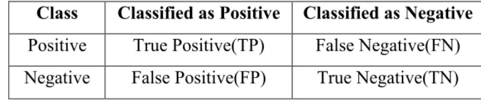
The results that have been evaluated in this experiment were the accuracy, the precision, the recall, the F-score and the time taken to build the model for each classifier, since the results should be extracted and evaluated in almost no time. Nevertheless, in order to give the explanation of accuracy, precision, recall and F-score, it is deemed necessary to present the confusion matrix as shown in Table 1 (Sokolova & Lapalme, 2009).
Table 1: Confusion Matrix
Class Classified as Positive Classified as Negative Positive True Positive(TP) False Negative(FN) Negative False Positive(FP) True Negative(TN)
Briefly, True Positive (or True Negative) means that a sample is in class Positive (or Negative) and correctly classified in the same class, while False Positive (or False Negative) means that a sample is in class Positive (or Negative) and it has been misclassified as Negative (or Positive).
According to the above, the accuracy, which is given by the following formula, is the number of instances that have been correctly classified, which means that if an
instance is in class Positive (or Negative), it is also classified in class Positive (or Negative). It can also be described with the following formula.
𝐴𝑐𝑐𝑢𝑟𝑎𝑐𝑦 = 𝑇𝑃 + 𝑇𝑁
𝑇𝑃 + 𝐹𝑃 + 𝑇𝑁 + 𝐹𝑁
In addition, precision is calculated with the formula below:
𝑃𝑟𝑒𝑐𝑖𝑠𝑖𝑜𝑛 = 𝑇𝑃
𝑇𝑃 + 𝐹𝑃
And it is the number of instances that correctly classified as Positives divided by the number of instances that the classifier has classified as Positives even if some of them are Negative.
On the same aspect, recall is given by the following formula:
𝑅𝑒𝑐𝑎𝑙𝑙 = 𝑇𝑃
𝑇𝑃 + 𝐹𝑁
And it is the number of instances that correctly classified as Positives divided by the number of all Positive instances.
At last, F-score is the combination of precision and recall and it is calculated as follows:
𝐹 − 𝑠𝑐𝑜𝑟𝑒 =2 ∙ 𝑝𝑟𝑒𝑐𝑖𝑠𝑖𝑜𝑛 ∙ 𝑟𝑒𝑐𝑎𝑙𝑙 𝑝𝑟𝑒𝑐𝑖𝑠𝑖𝑜𝑛 + 𝑟𝑒𝑐𝑎𝑙𝑙 6.4. Experimental results
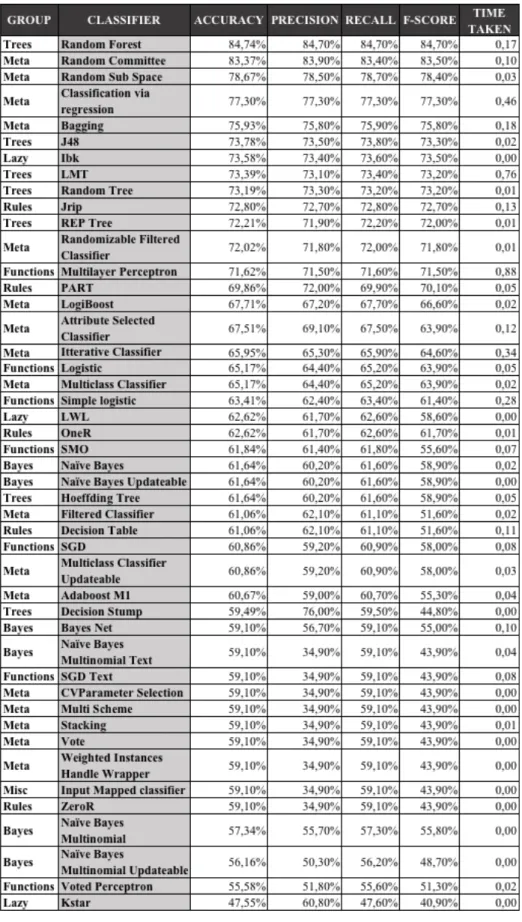
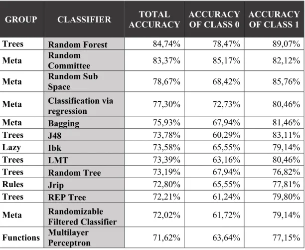
The first experiment was to evaluate all the available classifiers in Weka regarding the measures above with the given dataset intact. Also, the default parameters of each classifier were selected and as mentioned before the experiments were carried out with 10-fold cross validation (Bouckaert et al., 2016). The results are presented in Table 2 with a descending order from the classifier with the largest accuracy to the one with the smallest one.
Table 2: Classifier Results – Default Parameters – 10fold Cross Validation
As shown in the table above, 28.16% of the classifiers has an accuracy over 70%, 39.13% of them between 60% and 70% and 32.61% under 60%, while only 4.35%