Sever Institute
School of Engineering and Applied Science Department of Computer Science and Engineering
Dissertation Examination Committee: Ron K. Cytron, Chair
Steven Brams Jeremy Buhler Robert Pless
Itai Sened Aaron Stump
COMPUTATIONAL ASPECTS OF APPROVAL VOTING AND DECLARED-STRATEGY VOTING
by
Robert Hampton LeGrand III, B.S., M.C.S. A dissertation presented to the Graduate School of Arts and Sciences of Washington University in partial fulfillment
of the requirements for the degree of Doctor of Philosophy
May 2008 St. Louis, Missouri
Acknowledgements
I will always be grateful to my research advisor, Ron K. Cytron, for his guidance, perspective, encouragement and patience. He has been a pleasure to work with and a great help in exploring and evaluating research ideas and directions. I am passionate about this research and feel very lucky to have had the opportunity to work with him on it.
I also appreciate Steven J. Brams of NYU for his groundbreaking ideas that inspired much of this work. He has been extraordinarily encouraging and generous with his time, and it was a great honor to have him serve on my dissertation examination committee.
I would also like to thank the rest of my committee, Jeremy Buhler, Robert Pless, Itai Sened and Aaron Stump, for their time and valuable comments, and the DOC Group, especially James Brodman, Delvin Defoe, Morgan Deters, Scott Friedman, Richard Hough, Tobias Mann and Justin Thiel, who made it such a fun lab to work in.
Finally, for their love, support and pride, I owe my parents, Robert H. LeGrand Jr. and Marsha LeGrand, the most thanks of all.
Robert Hampton LeGrand III
Washington University, St. Louis May 2008
Contents
Acknowledgements . . . i
List of Tables . . . v
List of Figures . . . vi
Preface . . . ix
1 Introduction and Background . . . 1
1.1 Declared-Strategy Voting . . . 1
1.2 Approval voting . . . 4
1.3 Notions of sincerity . . . 5
1.4 Existing strategic approaches . . . 7
1.5 Computationally simple approval strategies . . . 9
2 Manipulation (or, What You Will) . . . 13
2.1 Notions of manipulation . . . 14
2.1.1 Election specification . . . 15
2.1.2 Ballot choice of voters . . . 15
2.2 Manipulation decision problems . . . 16
2.3 Strategic insincerity and DSV . . . 19
2.3.1 An NP-hard result . . . 19
2.5 Summary of contributions . . . 22
3 DSV and Approval-Rating Polls . . . 23
3.1 Approval ratings and their aggregation . . . 24
3.1.1 Examples of approval rating polls . . . 24
3.1.2 Formulation . . . 25
3.1.3 Aggregating approval ratings . . . 27
3.2 Rationally optimal strategy for Average aggregation . . . 31
3.2.1 Strategy for a final, omnisicent voter . . . 31
3.2.2 Equilibrium fornstrategic voters . . . 33
3.3 Multiple equilibria can exist . . . 36
3.4 At most one equilibrium average rating can exist . . . 37
3.5 At least one equilibrium always exists . . . 39
3.6 Average-Approval-Rating DSV . . . 47
3.6.1 A new class of rating systems . . . 49
3.6.2 Monotonicity of AAR DSV . . . 51
3.6.3 AAR DSV is immune to Average-style strategy . . . 52
3.6.4 AAR DSV never rewards insincerity . . . 55
3.7 A simpler AAR DSV algorithm . . . 58
3.8 Parameterizing AAR DSV . . . 62
3.9 Evaluation of AAR DSV systems . . . 64
3.10 Generalizations to more dimensions . . . 67
3.11 Summary of contributions . . . 70
4 Comparing Approval Strategies for DSV . . . 71
4.1 The space of approval ballots . . . 73
4.2 A new declared strategy for approval voting . . . 73 iii
4.3.1 Evaluating election states directly . . . 74
4.3.2 Evaluating election states by looking ahead . . . 77
4.4 General results using the Merrill election-state metric . . . 81
4.4.1 Comparing strategies A and T in the three-alternative case . . . 81
4.4.2 Comparing strategies A and J in the three-alternative case . . . 84
4.4.3 Comparing strategies T and J in the three-alternative case . . . 86
4.4.4 Comparing strategies A and Z in the three-alternative case . . . 89
4.4.5 Comparing strategies A and T in the four-alternative case . . . 92
4.4.6 A general result for strategy A using the Merrill metric . . . 99
4.5 General results using the branching-probabilities election-state metric . . . 100
4.5.1 A general result for strategy A using the branching-probabilities metric . . . 102
4.6 Summary of contributions . . . 104
5 Fixed-size Minimax . . . 106
5.1 Introduction . . . 106
5.1.1 Related work . . . 108
5.2 Definitions and notation . . . 109
5.3 NP-hardness and approximation algorithms . . . 110
5.4 Local search heuristics for fixed-size minimax . . . 112
5.4.1 A framework for FSM heuristics . . . 112
5.4.2 Evaluating the heuristics . . . 114
5.5 Manipulation . . . 116 5.6 Future work . . . 119 5.7 Acknowledgements . . . 120 5.8 Summary of contributions . . . 120 References. . . 121 iv
List of Tables
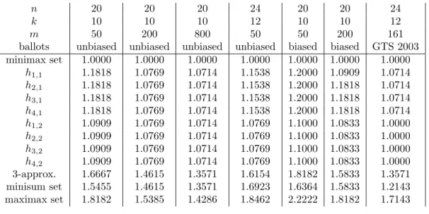
5.1 Largest approximation ratios found for local search heuristics . . . 115 5.2 Average approximation ratios found for local search heuristics . . . 116 5.3 Average scaled performance of local search heuristics . . . 117
List of Figures
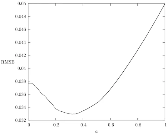
1.1 Outline of DSV operation . . . 2 1.2 Approval strategy Z . . . 10 1.3 Approval strategy T . . . 11 1.4 Approval strategy B . . . 11 1.5 Approval strategy J . . . 123.1 RMSE, varyingaand fixingb= 0.5000 . . . 65
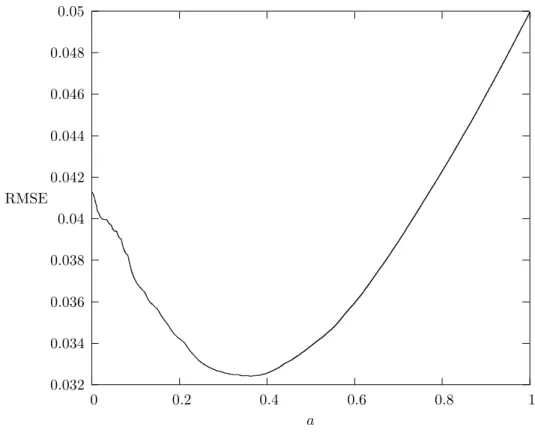
3.2 RMSE, varyingaand fixingb= 0.4820 . . . 66
3.3 RMSE, fixinga= 0.3647 and varyingb. . . 67
3.4 Φ0.3647,0.4820(~v) vs. ¯vscatterplot . . . 68
4.1 Approval strategy A . . . 74
Computational Aspects of Approval Voting and Declared-Strategy Voting
by
Robert Hampton LeGrand III
May 2008 Washington University
St. Louis, Missouri
Professor Ron K. Cytron, Chairperson
Computational social choice is a relatively new discipline that explores issues at the intersection of social choice theory and computer science. Designing a protocol for collective decision-making is made difficult by the possibility of manipulation through insincere voting. In approval voting systems, voters decide whether to approve or disapprove available alternatives; however, the specific nature of rational approval strategies has not been adequately studied. This research explores aspects of strategy under three different approval systems, from chiefly a computational viewpoint. While traditional voting systems elicit only the outcome of a voter’s strategic thinking, a
Declared-Strategy Voting (DSV) system accepts such strategies directly and applies them
according to the voter’s preferences over the available alternatives. Ideally, when rational strategies are employed on behalf of the voters, voters are discouraged from expressing insincere preferences. Approval voting is a natural fit for use with DSV, but, unlike for the common plurality voting system, there is no extant theory regarding the most effective approval strategies in a DSV context. We propose such a theory.
Approval-rating polls already serve an important role in assaying the views of an electorate on some subject of interest. Sites such as Rotten Tomatoes and Metacritic.com collect and display the results of approval-rating polls for movies and games. Moreover, sites such as Amazon and eBay
rational voter’s approval or disapproval will sometimes be insincere so as to move the result in a desired direction. A nonmanipulable protocol would allow indication of a voter’s ideal outcome and would never reward an insincere such indication. We present and analyze a large new class of such nonmanipulable protocols motivated by the DSV concept.
The minimax procedure is a multiwinner form of approval voting that aims to maximize the satisfaction with the outcome of the least satisfied voter. Unfortunately, computing the minimax winner set is computationally hard. We propose an approximation algorithm for this problem, a framework for polynomial-time heuristics that perform very well in practice, and a preliminary analysis of strategic voting under minimax.
Preface
Computer technology has been made to serve mankind in many ways. Today computers make simple many tasks that were previously more difficult or even impossible. Many public elections remained largely mechanical with little help from computers well into the information age, but computerized voting systems have received rapidly increasing attention since 2000 [40, 31]. Much has been written [3, 41] about real and theoretical computerized systems that verify voters, collect ballots and count votes, but there has been relatively little exploration of the possibility of
computers assisting voters with making strategic voting decisions.
When voting in elections, voters often find that a sincere ballot is unlikely to be the most effective one. For example, imagine an election for a single winner with three alternatives in which each voter is allowed to give a vote to one alternative. If a specific voter prefersAtoB andB toC, but estimates thatAis likely to finish a distant third, that voter may decide that choosingB is more likely to have a positive effect on the outcome. The outcome of an election can depend greatly on the extent and quality of this kind of strategically insincere voting in the electorate.
But choosing the most effective ballot is not always straightforward for a human voter, especially when the voter has little information on the alternatives’ relative strengths. Even when rich information regarding the current vote totals and other voters’ preferences is available, the most effective ballot—that is, the one that is likeliest to lead to the optimal reachable outcome—may not be obvious to a human voter. What is needed, then, is a system that will carry out the calculations required to find an optimally effective ballot for the voter. Such a system would make both na¨ıvely sincere and sophisticated voters equally effective.
Chapter 1
Introduction and Background
In this chapter we will introduce important concepts and review previous work relevant to our research directions.
1.1
Declared-Strategy Voting
In 1996, Lorrie Cranor and Ron K. Cytron [23] described a hypothetical voting system they called Declared-Strategy Voting (DSV). DSV arose from the desire to elicit richer, more sincere1
preferences from voters by using that information to find a winning alternative in such a way that voters would be unlikely to gain a superior result by submitting insincere preferences.
DSV can be seen as a meta-voting system, in that it uses voters’ expressed preferences among alternatives to vote rationally in their stead in repeated simulated elections. The repeated
simulated elections are run according to the rules of some underlying voting protocol, which can be any protocol that accepts any kind of ballots and uses them to elect one winner. Cranor [22] explored using DSV with plurality, but DSV, as a meta-voting system, could conceivably work with any voting protocol.
1Unfortunately, the terms “sincerity” and “manipulation” are used with little consistency in the social-choice
literature. We will review the various uses of these terms and define the senses in which we use them, “sincerity” in this chapter and “manipulation” in the next.
ballot vector
.
..
.
.
.
state election visible ballot current ballot processor executor state calculator program program program generators ("voters") program winner(s) program judge selectorFigure 1.1: Outline of DSV operation
As depicted in Figure 1.1, a DSV system maintains aballot vector and anelection state through a series of rounds. The ballot vector is empty at the beginning of the election and is updated after each voter’s program executes to hold all of the current ballots. The election state consists of a vector of rational numbers, one for each alternative in the election, that correspond to the current vote totals. It is updated using the ballot vector; the DSV mode (described below) of the election determines when and how that update takes place.
In a DSV election, a voter submits not a ballot but a DSVprogram. A program is essentially a function that takes some set of updated information about an election in progress as input and uses it to decide on a ballot to vote in the voter’s stead. In the most general case, the program itself can be any algorithm taking in all input related to the election in progress, such as all ballots previously voted, the contents of all other submitted programs and the number of ballots processed so far. But few real-world voters are sophisticated enough to provide such a program directly. In this research, a program is assumed to consist of a set of a voter’scardinal preferences (or utility ratings) over the alternatives and a rule, known as adeclared strategy, that generates an appropriate ballot at that point in the election. The cardinal preferences (ratings) are constrained to rational numbers between 0 and 1 inclusively; a rating measures the utility of an alternative to a voter—the degree to which that alternative’s victory is desirable. For example, if alternatives are candidates for public office, a rating can be interpreted as an estimate of the proportion of issues on which the voter and candidate agree, weighted by importance to the voter and likelihood of
relevance during the period of representation. Ratings are assumed to scale linearly and otherwise behave as von Neumann–Morgenstern utilities [57].
The declared strategy is a precisely defined algorithm that takes as input only the current election state, the voter’s cardinal preferences and the voter’s previously voted ballot; notably, the declared strategy has no knowledge of when it will next be executed or which voters’ programs have already executed. The declared strategy is expressed by submitting a well defined algorithm or choosing one from a predetermined list. The aim of the declared strategy is to maximize the result of the election according to the voter’s submitted cardinal preferences.
Once all programs are submitted, aselector selects a program to be executed. The selector effectively determines the order in which the programs are executed. Theithround consists of the
ith execution of each program and the processing of the resulting ballots. Each program must be selecteditimes before any program may be selected in round (i+ 1), but apart from that restriction the selection is random and impartial.
Anexecutor interprets the selected program and runs it with the current election state as input to produce a ballot as output. Only a finite number of computational steps is allowed to the program; if the program has not finished execution in the allotted number of steps, it is halted and an empty ballot results. This number can be made large enough for any reasonable program to complete comfortably but must be finite to guarantee progress and eventual completion of the election. The declared strategies considered in this research will be polynomial-time algorithms and will be assumed to finish in the allotted number of steps.
The ballot that is generated is then passed on to theballot processor, which checks whether the ballot is well formed according to the underlying voting protocol. For example, if plurality were being used as the underlying voting protocol, the ballot [1,1,0] would be rejected since plurality only allows one vote for at most one alternative. If the ballot is accepted as valid, the ballot processor then integrates it into the current ballot vector; the election’smode determines how that integration occurs.
The two modes described by Cranor [22] are ballot-by-ballot mode and batch mode. In this research, a mode can further benon-cumulative(like Cranor’s modes) orcumulative, giving four
possible DSV modes: ballot-by-ballot, batch, cumulative ballot-by-ballot and cumulative batch. If an election is run in one of the cumulative modes, the ballot processor adds a newly voted ballot to the ballot vector; if a non-cumulative mode is used, the ballot processor uses a newly voted ballot to replace that voter’s previously voted ballot, so that each voter has at most one ballot in the ballot vector at any time.
Thestate calculator uses the current ballot vector to update the election state; the election’s mode also determines how this update occurs. If the system is in a ballot-by-ballot mode, whether cumulative or not, the ballots in the ballot vector are summed and the summed vector replaces the previous election state after each ballot is processed. In a batch mode, the summed vector replaces the previous election state only after the last ballot of each round, that is, when each program has been executed the same number of times.
The underlying voting protocol (e.g., plurality), the mode (e.g., non-cumulative batch mode) and the number of rounds (e.g., 30) are the only settings needed to specify a DSV voting system fully.
1.2
Approval voting
Approval voting is a simple single-winner voting protocol. It was used in the Republic of Venice and to elect the pope in the thirteenth through seventeenth centuries [47], and it was rediscovered independently in the 1970s by several authors, including Guy Ottewell [44], Robert Weber [59] and Steven Brams and Peter Fishburn [13]. Under approval voting each voter may approve any subset of the available alternatives, effectively recording ayes orno vote for each alternative. In this version of approval voting that elects exactly one of a finite number of discrete alternatives, the one alternative that receives the most approval votes is chosen as the winner.
We propose that approval voting is a good candidate for use with DSV. DSV with plurality has been previously explored [22]; a plurality vote that can be expected to maximize a voter’s utility of the eventual outcome often deserts a favorite alternative to vote for another. More generally, it is sometimes rational to vote forA (and notB) even thoughB is preferred toA. Under approval voting a voter could vote fully for the same compromise alternative while also supporting fully his
or her favorite. Assuming the favorite has a nonzero chance of winning, doing so will further increase expected utility of the outcome, so perhaps approval voting induces less insincere voting by some measure. For example, unlike under plurality, it may never be rational under approval voting to vote forAand notB whenB is preferred toA.
1.3
Notions of sincerity
Under most voting systems,insincere voters can gain an advantageous outcome. Specifically, for most systems it sometimes happens that the most effective ballot contradicts a voter’s true preferences. For example, if a voter’s true preferences are forAoverB andB overCand the other votes total 40 forA, 50 forB and 50 forC, the single most effective plurality ballot is one forB. It is reasonable to consider such a ballot insincere because it expresses a pairwise preference forB
overA, contradicting the voter’s sincere preferences.
Standard since Arrow’s seminal impossibility result [4] in the realm of voting theory is to assume ordinal preferences and ordinal ballots. In such a world, a sincere ordinal ballot is simply one that exactly reflects the voter’s ordinal preferences. (Of course, if voters may have tied preferences, then they must be allowed to vote tied rankings to maintain the possibility of sincerity.)
This notion of sincerity can be generalized to cardinal preferences and ballots in different ways, but we focus on two in this work.2 First, If voters are assumed to have Von Neumann–Morgenstern [57] (cardinal and linearly scalable) utilities over the available alternatives, wherep(i) is a voter’s cardinal preference (utility) for alternativei, and any particular allowed ballot is interpreted to assign a ratingv(i) to each alternative, then at least two notions of sincerity can be easily defined:
strong sincerity A ballot is strongly sincere if and only if, for all alternativesiandj,
v(i)> v(j)←→p(i)> p(j).
2We assume that any voting protocol accepts ballots that can be interpreted to assign some rating to each
al-ternative. For example, plurality only allows assigning the rating 1 to one alternative and 0 to the rest; approval voting allows assigning either 0 or 1 to each alternative; ranked-ballot voting systems allow any assignment of rational numbers to the alternatives, where alternatives given higher ratings are taken to be ranked ahead of those given lower ratings. So cardinal-ratings ballots nicely generalize a large class of ballots without loss of information, though each voting protocol has its own set of allowed ballots.
weak sincerity A ballot is weakly sincere if and only if, for all alternativesiandj,
v(i)> v(j)−→p(i)> p(j). (This definition is equivalent to the definition of sincerity given by Brams and Fishburn [14, p. 29].)
So, for example, a voter with sincere utilities over three alternatives [1,0.8,0] might vote the approval ballot [1,1,0]; such a ballot is weakly but not strongly sincere. (Note that no strongly sincere approval ballot exists for a voter with tri- or multichotomous [14, p. 17] preferences such as these.)
Merrill [38, p. 80] outlines different notions of sincerity specifically for approval voting. He describes an approval ballot that is not even weakly sincere as askipping ballot, as such a ballot’s approvals “skip” down the voter’s preference ordering. For example, a voter who prefersAtoB to
C toD but approves onlyAandC is voting a skipping ballot. By this definition, an approval ballot is weakly sincere if and only if it is not skipping.
Notice that, if a voter knows exactly how every other voter will vote, a skipping ballot cannot be uniquely best. In other words, for any skipping ballot, there is some weakly sincere approval ballot that obtains an outcome which is no worse. For example, ifC andD are tied for the win, then, for the voter mentioned above, approvingB as well asAandC can only help; ifAandB are tied for the win, then approvingC as well asAcan only hurt.
Also specifically for approval voting, Merrill defines “pure” sincerity:
pure sincerity An approval ballot is purely sincere if and only if, for allk alternativesi,
p(i)> jp(j)
k −→v(i) = 1 and p(i)≤
jp(j)
k −→v(i) = 0.
Note that, according to this definition, if a voter assigns equal utilities to all alternatives, a purely sincere ballot would disapprove all alternatives.
Gibbard [30] and Satterthwaite [53] independently showed that, for any voting protocol that treats ballots and alternatives symmetrically, the most effective ballot is not always strongly sincere when there are at least three alternatives.3 The two protocols most often given as examples to which the 3The Gibbard–Satterthwaite theorem considers protocols with fully ranked input, so every weakly sincere ballot is
also strongly sincere. The theorem also effectively applies to protocols that accept ballots with tied ranks, but says only thatstrong (and not weak) sincerity must sometimes be violated by a rationally strategic voter.
Gibbard–Satterthwaite theorem does not apply arerandom ballot (a ballot is selected randomly; the highest rated alternative on it wins) andrandom runoff (two alternatives are randomly chosen; the one preferred to the other on more ballots wins). Neither treats ballots and alternatives symmetrically and thus are not generally considered appropriate for real-world elections.
So, every reasonable voting protocol sometimes rewards departing from strong sincerity, but, as we will further see below in section 1.4, approval voting can be said never to reward departing from weak sincerity. Other well-known protocols such as plurality, Hare (STV) [8] and Borda [51] cannot make the same claim.
1.4
Existing strategic approaches
While a DSV program can in general be any piece of code that a voter submits, rational
program-writers will be attempting to generate a ballot that takes their cardinal preferences into account. Accordingly, we have assumed that a program consists of (1) cardinal preferences over the alternatives and (2) a declared strategy, which uses the election state and the cardinal preferences to find a ballot that is deemed likeliest to maximize the election result according to the preferences. Several authors have investigated concepts very similar to what we call declared strategies. Brams and Fishburn [14, ch. 7] explore a concept they call the “poll assumption”, which models changes in voters’ strategy given the election state (the “poll”) under both plurality and approval voting. One variation, which they call the “Poll Assumption (Approval)”, is defined on page 115 (they use the term “strategy” to mean what we call “ballot”):
After the poll, voters will adjust their voting strategies [ballots] to distinguish between the top two candidates, as indicated by the poll [election state], if they prefer one of these candidates to the other and their sincere, pre-poll strategies did not involve voting for exactly one of these choices. Given that they are not indifferent between the top two candidates in the poll, they will vote after the poll for their preferred candidate and all candidates preferred to him (if any). [14]
Below (Figure 1.4) we will call this poll assumption “strategy B” and define it more precisely. Brams and Fishburn give examples that show alternatives being hurt and helped when voters strategically respond to poll information using this poll assumption; we will see that there exist other reasonable ways to respond to polls that may result in different equilibria when all voters use them.
Chapter 5 of Merrill [38] constructs a general theory of strategy under uncertainty (where nothing is known about the alternatives’ relative chances of winning) and risk (where each alternative’s probability of winning is assumed to be known or estimated). His approach to strategy under risk assumes knowledge of pivot probabilitiestij, wheretij is the probability that, given that the election results in a tie between two alternatives, alternativesiandj are the participants in the tie. He uses these pivot probabilities to calculate astrategic value for each alternative: the expected benefit according to the voter’s cardinal preferences of adding one vote for that alternative. He then finds, of all valid ballots, the one that maximizes the total strategic value. Cranor [22] offers a theory of rational declared strategies and applies it especially to plurality DSV elections. She outlines several approaches to transforming an election state into pivot probabilities, the most prominent of which essentially treats each alternative’s proportion of the votes in the current election state as the mean of a Gaussian distribution of that alternative’s eventual
proportion of the votes, assumes some particular variance for the distribution (S2, which could be seen as a measure of uncertainty in the current vote totals), and then calculates the probability that each pair of alternatives will eventually tie for the win. When voters are randomly sampled to obtain the distribution, the variance can be modeled according to the Gaussian error of estimate based on the fraction of the electorate sampled so far. The resulting pivot probabilities are then used as by Merrill to find an optimal plurality ballot.
Cranor’s approach attempts to define rational strategy directly by making certain reasonable assumptions but does not atttempt to show that, in practice, the strategies found lead to better results for voters that use them than any other strategy approaches.
1.5
Computationally simple approval strategies
Several existing styles of designing effective declared strategies were described in section 1.4. Some, such as the strategies of Brams and Fishburn, were intended to model approximately how typical real-world voters might vote when they have poll information. Such strategies are desirable for DSV for three reasons: they are based on results that have already appeared in the literature, they can be described simply enough for a human voter to understand easily and they can be executed quickly by a computer regardless of the numbers of voters and alternatives. Several such strategies are defined below; they all are computationally simple and can be found in extant literature. All of them always result in a weakly sincere approval ballot, essentially setting some cardinal cutoff over which alternatives are approved and under which they are disapproved, so skipping ballots never result.
To simplify the description of approval strategies, we will assume that DSV is run in
non-cumulative batch mode, which means that the election state visible to a voter in roundr+ 1 depends only on the ballots submitted in roundr.
Notation varies widely in the literature, but we will describe election situations using the following. Any election hask alternatives numbered from 1 tok andnvoters numbered from 1 ton. For notational convenience, nis defined as the set{z∈ : 1≤z≤n}(the integers between 1 andn) and m...nis defined as the set{q∈ :m≤q≤n}(the rational numbers betweenm andn).
The voters’ sincere cardinal preferences are represented as the functionp: n× k→ , where p(i, j) = voteri’s cardinal preference for alternativej. The ballots submitted throughout the DSV rounds are represented as the functionb: n× k× → 0...1, whereb(i, j, r) = voteri’s vote for
alternativej in roundr;b(i, j,0) = 0 for all iandj.4 The election states are represented as the functions: k× → 0...n, wheres(j, r) =
Pn
i=1b(i, j, r), alternativej’s vote total at the end of roundr.
The approval strategies defined below calculate the ballot for voterv at roundr+ 1; that is, given
v andr, they calculateb(v, i, r+ 1) (= 1 for approval and 0 for disapproval) for each alternativei. 4Here
It will be useful to define two more functions. Topy(r) is the set of they leading alternatives according to roundr’s election state:
Topy(r) ={i:|{j:s(i, r)< s(j, r)}|< y}
PSumy(v, r) is the sum of voterv’s cardinal preferences of the alternatives in Topy(r):
PSumy(v, r) = X j∈Topy(r)
p(v, j)
Also, we define the setC(r) of “contending” alternatives at roundrto be {i:s(i, r)≥x}wherex
is as large as possible with the constraint that|C(r)| ≥2 for allr.
One of the simplest strategies effectively ignores the election state and assumes that each alternative has an equal probability of winning the election, approving each alternative the voter rates higher than his average rating over all alternatives. We call this approach strategy Z and define it precisely in Figure 1.2. Note that the definition uses Top and PSum to make clear its similarities with those of the other strategies we will consider, but as only Topk and PSumk are used the effect is to compare each alternative’s utility to the average utility over all the
alternatives, so the election state is effectively ignored.
Figure 1.2: Approval strategy Z For voterv voting in roundr+ 1,
• for each alternative i:
– approve alternativeiif and only ifp(v, i)· |Topk(r)|>PSumk(v, r)
Strategy Z is always purely sincere according to Merrill’s definition above. It is also equivalent to the optimal approval strategy according to the Laplace method for making decisions under uncertainty Merrill [38] gives in chapter 5.
Another strategy based only on a voter’s preferences and the alternatives’ current vote totals is often given by advocates of approval voting as a good rule of thumb for real-world approval elections [47, p. 196]. Mike Ossipoff [43] wrote, “In Plurality, if you’re sure that Smith & Jones will be the top 2 votegetters, then obviously you should vote for whichever of those 2 you prefer to the
other. In Approval, vote for him and for everyone whom you like better.” Equivalently, an
approval cutoff is placed just below the preferred of the top two alternatives. We call this approach strategy T and define it more precisely in Figure 1.3.
Figure 1.3: Approval strategy T For voterv voting in roundr+ 1,
• for each alternative i:
– find smallesty such thatp(v, i)· |Topy(r)| 6= PSumy(v, r) (y=kif none)
– ify≤2:
∗ approve alternative iif and only if p(v, i)· |Top1(r)| >PSum1(v, r) andp(v, i)·(|Top2(r)| − |Top1(r)|)>PSum2(v, r)−PSum1(v, r)
– else:
∗ approve alternativeiif and only ifp(v, i)· |Topy(r)|>PSumy(v, r)
The first of the two strategies Brams and Fishburn [14] describe we will call strategy B; the second we will call strategy J. Strategy B takes as input not only a voter’s preferences and the
alternatives’ current vote totals but also the voter’s previous ballot. We use the description of the Poll Assumption (Approval) and the ensuing examples to inspire the precise definition of Strategy B in Figure 1.4. Strategy B will change a voter’s ballot only when necessary to differentiate among the contending alternatives.
Figure 1.4: Approval strategy B For voterv voting in roundr+ 1,
• ifr >0:
– b−1= voterv’s ballot cast in roundr • else:
– b−1= ballot found by applying strategy Z
• ifb−1includes all alternatives inC(r) ornone of them:
– apply strategy T • else:
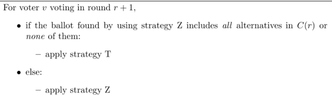
Brams and Fishburn describe a variation on their Poll Assumption (Approval) on page 120, which can be generalized to what we call strategy J and define precisely in Figure 1.5. Strategy J will vote a purely sincere ballot whenever doing so would differentiate among the contending alternatives.
Figure 1.5: Approval strategy J For voterv voting in roundr+ 1,
• if the ballot found by using strategy Z includes all alternatives in C(r) or none of them:
– apply strategy T • else:
– apply strategy Z
It is worth pointing out that the approval strategies presented above (plus strategy A, defined in Figure 4.1) effectively use only the ordinal preferences of a voter. In other words, any cardinal preferences that impose the same preference order over the alternatives will result in identical ballots if any of these strategies is used. Therefore they can be used equally effectively whether preference input consists of cardinal utilities or a (perhaps partial) ordering of the alternatives. In chapter 4 we will compare the effectiveness of these approval strategies according to different evaluation metrics.
Chapter 2
Manipulation (or, What You Will)
The developers [23] of Declared-Strategy Voting (DSV) elections posited that their election protocol would force rational voters to specify cardinal preferencessincerely, while still acting in the best interest of each voter at the moment that voter must pick an alternative. In this way they were attempting to avoid the possibility ofmanipulation, which is an unfortunately grossly
overloaded term in voting literature. In section 2.1, we examine the nature of manipulation in voting systems, settling on a definition that suits our goals in this chapter.
The act of voting requires brain activity, and the Church–Turing hypothesis [18, 55, 33] says that activity can be captured by a program. That programP takes in basically three things: the election protocol, the voter’s feelings about the alternatives and the voter’s expectations concerning how everybody else will vote.
The protocol specifies the manner in which the election will be conducted: it is a mathematical function from a list of ballots to one or more winners. We assume that voters cannot (will not) act until the protocol has been set. With the protocol established, a voter will act based upon the other two factors: that voter’s feelings about the alternatives, and that voter’s expectation concerning how everybody else will vote.
sincerity IfP is based only on the voter’s feelings, ignoring how others might vote, thenP is actingsincerely. However, it is well known [30, 53] that acting so directly on the voter’s feelings may result in a provably worse outcome for the voter in terms of who wins the election. In that sense,P is generallyirrational and a better outcome is obtainable through strategic behavior.
irrationality IfP is based only on how others vote, ignoring how the voter feels about the alternatives, thenP is by definitionirrational. Examples include bandwagon and underdog voting [22].
strategy IfP takes into account both how the voter feels and how others might vote, thenP is actingstrategically (even thoughP may happen to output a ballot that is sincere in some sense). IfP can be shown, by some objective measure perhaps similar to those explored in chapter 4, to obtain outcomes influenced favorably by the voter’s preferences, thenP can be said to be actingrationally.
In summary of DSV, most voting protcols compel voters to act strategically to be rational. DSV elections hope to cause voters to actsincerely to be rational—by moving the voter’s insincere program into the DSV system itself.
2.1
Notions of manipulation
One of a democracy’s goals is to conduct elections that arefair, in the sense that no individual has anundue influence on an election’s outcome. Such influence is loosely calledmanipulation, and we next examine various mechanisms by which an individual (or group of collaborating individuals) can influence an election’s outcome. Of course, every voter has the potential to influence an election’s outcome; otherwise, voting would be a futile activity. In discussions of manipulation, it is therefore important to discern the nature of influence and to establish the conditions under which an individual’s influence is unfair.
2.1.1
Election specification
Those who specify an election and its protocol have the ability to manipulate an election. For example, election officials could overtly exclude an alternative, either so that alternative cannot win or because, if included, that alternative would prevent the election of a more desirable alternative due to a vote-splitting effect [42]. They could also affect the outcome by determining the set of allowed voters [9], perhaps allowing only those who support the favored outcome or excluding those who support strong rival outcomes. More subtly, if the election officials have the chance to choose an election protocol, then one can be chosen so as to obtain (probabilistically or for certain) a given outcome [52], or at least one that is less likely to give a particular undesirable outcome.
2.1.2
Ballot choice of voters
More common in the literature is to identify the manipulation opportunities of voters themselves. Intuitively speaking, manipulation by a voter occurs when he or she changes a ballot in the expectation of effecting a superior outcome; in this research, we will use only this notion of manipulation. But when, more precisely, can manipulation be said to have occurred? We will consider two possibilities:
1. A voter or group of voters, using all available information, decides whether a specific alternative can be made to win with at least a given probability and, if so, votes in such a way to elect that alternative. (Such voters are actingstrategically in the sense defined above.) 2. A voter submits an insincere ballot that results in an election outcome better for that voter
than the one that would have resulted if he or she had voted sincerely. (Insincerity can be reckoned by weak sincerity or strong sincerity as defined in chapter 1.)
These two notions of manipulation addressstrategy andinsincerity, respectively.
The first is useful to consider when a voter is deciding how to vote; if a corresponding decision problem is shown to be computationally hard, it may be reasonable to expect voters to default to voting sincerely. Decision problems of this sort will be investigated in the next section.
The second identifies when a voter has “gamed the system”; it is what many social-choice authors mean when they describe a voting system as manipulable. (By this definition, a voting system is nonmanipulable when any rationally strategic ballot is sincere.) One design motivation for DSV was to encourage the submission of sincere preferences. In particular, it was hoped that
ballot-by-ballot mode, by randomizing voter order, would deter the submission of insincere preferences; if a voter determines that insincere preferences will gain a superior outcome given one voter order, the same preferences may be unlikely to gain the same outcome given another voter order.
2.2
Manipulation decision problems
There have already been attempts to characterize the difficulty of manipulating voting systems. The following decision problem is a generalization of several in the literature.
Existence of Probably Winning Coalition Ballots (EPWCB)
INSTANCE: Set of alternativesA and a distinguished memberaofA; set of weighted cardinal-ratings ballots BV; the weights of a set of ballotsBU which have not been cast; probability 0< π≤1
QUESTION: Does there exist a way to cast the ballots BU so thatahas at least probabilityπ of winning the election with the ballotsBV ∪BU?
EPWCB is perhaps best explained by presenting its interesting subproblems.
Existence of a Winning Ballot (EWB)
INSTANCE: Set of alternativesA and a distinguished memberaofA; set of cardinal-ratings ballots B
QUESTION: Does there exist a way to cast a ballot b0 so thatawins the election with the ballotsB∪ {b0}outright?
EWB is identical to the decision problemExistence of a Winning Preference (EWP)
standard for the literature in this area. EWB essentially looks at a manipulation opportunity from the point of view of a DSV voter coming last in the voter order: All other ballots are considered to be cast, fixed and known, and the question is whether there is a ballot that the ultimate voter can cast to cause the election of a certain alternative. The assumed situation is very much like that of a DSV program computing the final ballot of a round on behalf of its voter. Bartholdiet al.’s reasoning for using EWP is that it assumes all relevant information is available—if one can show that, for a given voting system, EWP is computationally hard, then manipulating that voting system must be hard when less information is available.
Bartholdi, Tovey and Trick are able to show that a polynomial-time algorithm exists for solving EWP in general for a large class of voting protocols, which includes plurality and approval voting. However, they present a protocol they call Second-Order Copeland for which solving EWP is NP-hard, and in a later paper Bartholdi and Orlin [8] show that EWP is also NP-hard for the single transferable vote (STV) in its single-winner version—also known as Hare, Instant Runoff Voting (IRV) or the alternative vote. But when the number of alternatives is held constant, a polynomial-time algorithm solving EWP exists even for these protocols, so EWP’s NP-hardness depends on a large slate of alternatives.
Existence of Winning Coalition Ballots (EWCB)
INSTANCE: Set of alternativesA and a distinguished memberaofA; set of weighted cardinal-ratings ballotsBV; the weights of a set of ballotsBU which have not been cast QUESTION: Does there exist a way to cast the ballots BU so thatawins the election outright?
EWCB isConstructive Coalitional Weighted Manipulation (CCWM), introduced by Conitzer and Sandholm [20], with cardinal instead of ordinal ballots as input. EWCB is a generalization of EWB that, surprisingly, is NP-hard for many protocols even given a constant number of alternatives.
Note that EWB and EWCB ask whether a specific alternative can be made to win. The more general and perhaps more intuitively useful problem of finding a voter’s most-liked alternative that can be made to win is not significantly harder: one would simply test each alternative in decending
order of cardinal preference; when alternativeacan be made to win, alternatives not preferred toa
need not be considered.
Conitzer and Sandholm [21] described three “tweaks” that, when added to a voting protocol, such as plurality or the Borda count [51], make that protocol computationally hard to manipulate. All three use a “preround” to determine a set of alternatives to be eliminated before the voting protocol is executed. The simplest, called a deterministic preround, publishes a pairing of the alternatives before the ballots are collected; for each pair, the loser of the pairwise comparison between them according to the ballots is eliminated—if the number of alternatives is odd, one alternative survives without a comparison—and the original protocol, such as plurality or Borda, is executed on the ballots over the remaining alternatives. Adding this deterministic preround to a large class of protocols, including plurality and Borda, renders them NP-hard to manipulate in the sense of EWP.
The second preround tweak pairs the alternatives randomly after the ballots have been collected; it makes a protocol #P-hard to manipulate, but in a special sense: Instead of asking whether a specific alternativeacan be made to win, as in EWP, it asks whetheracan be made to win with some given probability 0< π≤1.
Existence of a Probably Winning Ballot (EPWB)
INSTANCE: Set of alternativesA and a distinguished memberaofA; set of cardinal-ratings ballots B; probability 0< π≤1
QUESTION: Does there exist a way to cast a ballot b0 so thatahas at least probabilityπ of winning the election with the ballotsB∪ {b0}?
Perhaps the nondeterminism of DSV’s ballot-by-ballot mode has a similar effect on manipulation, either making it computationally difficult in this probabilistic sense or making it so that any manipulation that would work given one voter order would backfire for some other voter order. Recall from section 1.3 that the Gibbard–Satterthwaite theorem proves that any voting protocol, including a meta-voting system like DSV, that treats ballots and alternatives symmetrically is manipulable by strategic voters, and, further, that the two protocols (random ballot and random
runoff) most often given as examples to which the Gibbard–Satterthwaite theorem does not apply have a large nondeterministic component. Could it be that there is generally a tradeoff between manipulability and determinism?
2.3
Strategic insincerity and DSV
One motivation for the design of DSV was to elicit the submission of sincere preferences by having the system strategize for the voter. The hope is that the voter’s declared strategy will cast ballots in such a way that the eventual outcome of the election is optimized from the voter’s point of view, giving the voter no reason to try to gain a better outcome by submitting insincere preferences. In other words, one hopes that the declared strategy will do everything in its power to make the winner of the election as good as possible so that submitting false preferences can only backfire. Unfortunately, the Gibbard–Satterthwaite theorem dashes hope that any reasonable voting system will be found that is immune to strategic insincerity in all voting situations with at least three alternatives. So even DSV, assuming no bias towards some voters or some alternatives is built in, will have cases with opportunities for manipulation by submitting insincere cardinal preferences. Different DSV systems—those with different underlying voting protocols and in different
modes—may in practice present manipulation opportunities to voters more or less often. For example, it may be much easier to find an election example where plurality DSV rewards the submission of insincere cardinal preferences than for approval DSV. But even if DSV is sometimes manipulable, one might expect it to be generally difficult to find the preferences that would manipulate successfully.
2.3.1
An NP-hard result
As it turns out, DSV can be shown to be computationally hard to manipulate in a certain sense. EWB, the version of Bartholdi’s and Orlin’s [8] EWP with cardinal-preference ballots, captures the relevant notion of manipulability. They showed that EWP is NP-hard for Hare, the single-winner form of STV.
Hare takes ordinal ballots as input. The ballots are counted in a series of elimination rounds. In the first round, only the top-rank votes are counted. The alternative with the smallest top-rank total is eliminated from the ballots, possibly adding to other alternatives’ top-rank totals. This step is repeated until exactly one winner is left.
If a specific choice of declared strategy is forcibly made for all voters, DSV in batch mode with plurality as the underlying voting protocol can be made to simulate Hare. If the imposed declared strategy is carefully chosen, DSV can be made to select the winner that Hare would given the ranked ballots corresponding to the voters’ expressed cardinal preferences. So if voters are not free to choose their own declared strategies, DSV can be made NP-hard to manipulate.
Theorem 2.3.1. If a declared strategy can be imposed on the voters, so that they submit only their cardinal preferences over the alternatives, DSV can be made to be NP-hard to manipulate in the EWB sense.
Proof. We will always elect the Hare winner according to the ordinal ballots implied by the voters’ cardinal preferences if we use DSV in batch mode with one-vote plurality as the underlying protocol and the following strategy for all voters:
vote for alternativei such thatpi= max(pj :sj ≥t)
where t= min(U\ {min(U)}) if |U|>1 min(U) if |U|= 1 0 if |U|= 0 and U ={sj:sj >0}
In the first round of the batch DSV election, when (∀i)si = 0, the imposed strategy will vote for each voter’s favorite alternative, just as in the first round of counting a Hare election. In
subsequent DSV rounds, as long as|U|>1 (there remain more than one uneliminated alternative), all voters vote for their most preferred alternative with a vote total at leastt, a threshold set at the second-smallest vote total, effectively eliminating the alternative(s) with the lowest vote totals
among the uneliminated alternatives. When|U|= 1 (only one alternative has a nonzero vote total), every voter votes for that alternative. The resulting election state does not change afterward, and that alternative, which is the Hare winner, thus wins the DSV election. Bartholdi and Orlin [8] proved that Hare (the single-winner version of STV) is NP-hard to
manipulate in theExistence of a Winning Preference (EWP)sense. EWP is a subproblem of Existence of a Winning Ballot (EWB), so Hare is NP-hard to manipulate in the EWB sense as well. Since batch DSV with the above imposed strategy is equivalent to Hare, DSV can be made NP-hard to manipulate in the EWB sense.
So DSV is NP-hard to manipulate in the general case. But what does this mean? It means only that there is no algorithm that runs in time polynomial in the number of alternatives and the number of voters that is guaranteed to find a set of preferences that guarantees a given outcome. It doesnot mean that DSV is necessarily hard to manipulate in every case. There may be a simple heuristic that often (if not always) finds preferences that will manipulate successfully, or one that tends to lead to a better outcome than blind sincerity. It also does not imply that manipulating DSV is necessarily easy or hard when declared strategies can be freely chosen.
2.4
Generalizing hardness results to approval voting
Conitzer and Sandholm [19] showed that CCWM is in P for plurality for any constant number of alternatives but NP-hard for Borda and veto voting with three or more alternatives. (For every voting system under consideration, CCWM is in P when the number of alternatives is limited to two.) CCWM takes ranked ballots as input, so approval voting cannot be applied to CCWM. But EWCB works with approval voting; it is simply CCWM with cardinal-preference input. EWCB can be seen to be in P for approval voting by using the same manipulation algorithm that works for plurality: Approve on all ballots onlya, the distinguished alternative that is to be made to win. There is a way to makeawin if and only if this strategy makesawin.
2.5
Summary of contributions
In this research, we have accomplished the following.
1. Proved that manipulating DSV in general is NP-hard by describing a plurality DSV system that imposes a specified declared strategy on all voters in such a way that the Hare winner is elected.
Chapter 3
DSV and Approval-Rating Polls
We see DSV as a way to reduce or eliminate manipulation by voters’ insincerity by embracing manipulation itself. By strategizing for the voter, a “perfect” DSV system would encourage sincere indication of preferences. In the next chapter we will investigate questions regarding the
manipulability of DSV in the general case, where it is used to elect one of a static set of
alternatives over which voters may hold any preferences. But the DSV framework can be used in other contexts. In particular, if certain assumptions are made about the available alternatives and the voters’ preferences among them, stronger results regarding DSV are possible.
In this chapter we will investigate applying DSV to the problem of selecting a number from a specified range of numbers. We will show that this new application of DSV achieves the original goal of DSV: It eliminates the possibility of manipulation by making insincere voting no more effective than sincere voting. Intuitively, this is possible because we assume that voters can only have certain kinds of preferences over the possible outcomes, effectively reducing the space of possible elections. For example, if the alternatives consist of the rational numbers between 0 and 1, we can justifiably assume each voter’s preferences over the considered range to be single-peaked. In other words, we can assume that no voter will preferaoverb andc overbifa < b < c.
This application of DSV may have fewer uses in real-world elections than a more general DSV system that allows arbitrary voter preferences over alternatives, but it can be seen as an illustration of the power of DSV in principle and an ´etude for the further study of DSV.
3.1
Approval ratings and their aggregation
Approval ratings are one mechanism that communities can use to offer incentive and reward for good behavior or service. The prospect of feedback following a given interaction presumably increases the accountability of that interaction for all parties involved. Publication of approval ratings then enables appropriate consequences to follow from positive or negative experiences. It is interesting, however, to consider the form in which approval ratings can and should be published. While the greatest detail is afforded by publication of each participant’s response to an approval rating poll, the resulting volume is typically unacceptable for the purposes of
summarizing an electorate’s experience. Thus, some form of aggregation is typically performed on approval ratings, and the result of that aggregation is then announced as the result of the poll. In this chapter we consider several forms of aggregation and we show that some methods can reward insincerity while others cannot. We next provide several examples of approval rating systems and formulate a general form of an approval rating poll.
3.1.1
Examples of approval rating polls
Subscribers and observers of media frequently learn of the results ofapproval rating polls that attempt to discern how strongly a participating electorate endorses a person or a position of interest. For example, approval ratings concerning the performance of the United States President are published throughout a presidency; following events or policy decisions that affect an
electorate, such polls are often conducted as a means of evaluating the electorate’s support for the President’s actions.
As another example, several web sites post varous forms of approval ratings for movies and games. Specifically, Rotten Tomatoes [2] posts the results of two polls for each movie:
• Each review from a set of accredited critics is turned into approval (fresh rating) or
disapproval (rotten rating) of the reviewed material, in terms of whether the material merits viewing. The percentage of fresh reviews is reported as the movie’sTomatometer. In effect, each review is turned into a 0 or 1 value, and the Tomatometer is the average of those values expressed as a percentage. Putative viewers might consult a movie’s Tomatometer value to determine whether they should see that movie.
• Each critic can also rate a movie’s overall quality on a 1–10 scale. Rotten Tomatoes then publishes the average of all such ratings. Similarly, Metacritic [1] computes a weighted average of its accredited reviewers’ approval ratings for a given movie, supplied on a 0–100 scale.
Finally, consider the electronic marketplace, in which participants are asked to rate the honesty and effectiveness of merchants and customers. Sites such as eBay poll their participants concerning how strongly they approve of the behavior of the marketplace members they encounter in
transactions. Upon completion of a transaction, the involved parties are asked to rate each other. An aggregation of an indvidual’s approval ratings is posted for public view, so that members can consider such information before engaging that individual in a transaction.
Based on the above, some approval ratings are formulated more incrementally than others. For example, the ratings published by Rotten Tomatoes and Metacritic are collected and then analyzed en masse, while the approval rating of an eBay participant (merchant or customer) can be updated after every interaction involving that participant. As we show below, knowledge concerning how others approve of a given issue can influence a particpant’s expressed approval rating.
3.1.2
Formulation
• An electorate of nparticipants is polled. Based on the participants’ response and the aggregation protocol at hand, the result of the poll will be published as a rational number in the interval [0,1].
• Each participantihas in mind a sincere preference ratingri,0≤ri≤1 that can be construed as that participant’s dictatorial preference. The tuple of all participants’ sincere ratings is denoted by the vector~r.
We further make the reasonable assumption that voter i’s preferences are single-peaked and non-plateauing: a voter’s utilities for the outcomes are monotonically decreasing when moving away fromri in either direction. It follows, for example, that any voter that prefers 0.2 to 0.5 must also prefer 0.5 to 0.8. More formally:
– Ifa < b≤ri, then voteri must preferb toa;
– Ifri≤c < d, then voterimust preferc tod.
Based on the above,ri sufficiently characterizes a voter’s outcome utilities for our purposes. • Each participantihas also in mind a probability density functionpi that models the
probabilistic outcome of the poll, excluding i’s rating. For the purposes of this chapter, the outcome fromi’s point of view is simply an expected valueoi. While a more general
treatment could be the subject of future work, we therefore assumepi is the Diracδfunction:
pi=δ(t−oi) = ∞ if t=oi 0 if t6=oi with the area under pi summing by definition to unity.
– In situations where preference data accrues incrementally and the poll’s results are updated continually,oi is readily available before theith participant expresses approval. Such is the case in eBay when a buyer provides an approval rating for a merchant.
– In other cases, preliminary polls or other information sources may provide sufficient information to provide a likely value foroi.
While estimations ofoi could be inaccurate, faulty or based on purposefully falsified information, the presence of such information can affect an electorate as discussed below.
• Finally, voteriparticipates in the poll by expressing a rating preference of vi, which may or may not be the same asri. In fact, we are particularly interested in situations wherevi6=ri due to pi. For example, the expression of an individual’s approval rating could well be affected by knowledge (perceptions, estimations, or actualities) of how others approve of the issue at hand. For example, consider an eBay customer who undertakes a transaction with a highly approved merchant. If the customer becomes disgruntled with the merchant, then the customer’s resulting rating of the merchant might be overly negative, precisely because of the merchant’s otherwise high rating.
The tuple of all expressed approval ratings is denoted by the vector~v.
This chapter considers an approach that can account for, mitigate, or prevent the use of insincerity to increase a participant’s effectiveness in an approval rating poll.
3.1.3
Aggregating approval ratings
The results of an approval rating poll are typically reported by an aggregation procedure that is discloseda priori. In this section, we consider two popular aggregation schemes: average and median.
Average aggregation Here, the result of the approval rating poll is computed as the average of the participants’ expressed approval ratings:
¯
v=
Pn
j=1vj
n
While the Average aggregation function is sensitive to each voter’s input, it has an important disadvantage: Voters can often gain by voting insincerely. For example, the 1983 filmVideodrome has five critics’ ratings on Metacritic. If we assume that these critics rated the film sincerely (that each would prefer that the average rating of the film be his or her rating), we have
If these preferences are actually expressed sincerely in an Average aggregation context, then we have
~v= [0.4,0.7,0.8,0.8,0.88] and the Average aggregation yields 0.716.
Consider voter 5, whose ideal outcome isr5= 0.88. That voter could achive a better outcome by not expressing the sincere preferencev5= 0.88 and instead votingv5= 1. The resulting Average aggregation yields the outcome 0.74, which, being closer to 0.88, is preferred by voter 5 to 0.716.
Median aggregation (nodd) Another possible aggregation function computes amedian of~v: ˜
v is a value that satisfies
|{i: ˜v < vi}| ≤n 2 and |{i: ˜v > vi}| ≤ n 2 or, equivalently, |{i: ˜v < vi}| ≤ n 2 ≤ |{i: ˜v≤vi}|
The above definition does not necessarily prescribe a unique aggregation whennis even; we address this issue below.
According to themedian voter theorem [10, 24], whennis odd, Median aggregation becomes the unique, Condorcet-compliant [38] rating system, yielding a result that is preferred by some majority of voters to every other outcome.
Unfortunately, Median aggregation can effectively ignore almost half of the voters. In other words, majority rule can mean majority tyranny. Given the following tuple of votes
~v= [0,0,0,1,1]
the 1-voters are effectively ignored when the median, 0, is chosen as the outcome. Majority tyranny could be quite undesirable for polls of this type, especially when the goal of aggregating ratings is to represent a satisfactory consensus for all voters. The Average outcome of the above tuple, 0.4, arguably provides such a much better consensus.
In contrast with Average aggregation, Median aggregation is nonmanipulable by insincere voters—at least whennis odd: a voterican never improve the outcome from his or her point of view by votingvi6=ri.
Theorem 3.1.1. Whennis odd, each voteri obtains his or her best outcome by voting vi=ri.
Proof. Consider the relation of any voteri’s sincere preferenceri to the Median outcome ˜v, with the following three cases:
• ri= ˜v. Withi’s sincere preference as the outcome, no better result could obtain by changing
ri.
• ri<v˜. Becausenis odd, the median vote is uniquely determined. Thus, decreasingri cannot affect ˜v; increasingri could only increase ˜v, which would produce a less desirable outcome for voteri.
• ri>v˜. A symmetric argument based on the above holds here as well.
Thus, Median aggregation does not reward insincerity for an odd number of participants.
Median aggregation (generalized) The conventional method in statistics for computing the Median of an even number of values is to compute the average of the middle two values. In such a situation, the voter who cast one of those two values could pull the outcome in a beneficial direction by voting insincerely.
Fortunately, there are many methods to eliminate such manipulation; examples include the following:
• One of the two middle values could be chosen at random.
• If 0.5 lies between the two middle values, then 0.5 is chosen; otherwise, the one of the two that is nearer 0.5 is chosen.
Note that the outcome ˜v given by any of these median functions minimizesP
i|vi−v˜|, in contrast to the average function, ¯v, which minimizesP
i(vi−¯v)2.
Without losing nonmanipulability, the Median function can be generalized to give the outcome
b˜v where |{i:b˜v < vi}| ≤bn≤ |{i:b˜v≤vi}|
for any 0≤b≤1. (In this notation, theb is intended as a parameter modifying the tilde.) Ifbn is an integer, there may be more than one 0≤φ≤1] that satisfies
|{i:φ < vi}| ≤bn≤ |{i:φ≤vi}|
In that case, define Φ as the set of all suchφ. Then
bv˜≡ min(Φ) if b <min(Φ) b if min(Φ)≤b≤max(Φ) max(Φ) if max(Φ)< b or, equivalently, b˜v≡ min(Φ) if (∀φ∈Φ)φ > b b if b∈Φ max(Φ) if (∀φ∈Φ)φ < b
This order-statistic outcome equals max(~v) whenb= 0, the third quartile whenb= 1
4, the Median outcome whenb= 12, the first quartile whenb= 34 and min(~v) whenb= 1.
Summary For an approval-rating poll, the choice of aggregation mechanism affects the nature of the outcome and the reward for voter insincerity. The Average aggregation outcome can reward insincerity, but the outcome provides a reasonable consensus of the electorate. On the other hand, Median aggregation does not reward insincerity, but it allows for tyranny by a majority.
3.2
Rationally optimal strategy for Average aggregation
As shown in section 3.1, Average aggregation can reward insincerity. In this section, we develop a rationally optimal strategy: a computation by which a voter can achieve a result as close as possible to that voter’s prefered outcome. As before, we assume an eletorate in whichnvoters will express preferences. We begin by considering a rationally optimal strategy from the perspective of a final, omniscient voter. We then consider the behavior of a system in which all voters use a rationally optimal strategy.
To facilitate exposition and analysis of our results, we begin by generalizing the scale on which preferences are expressed as follows. In an [m, M]-Average poll, voters are allowed toexpress preference ratings in the interval [m, M], m≤0,1≤M. We continue to assume thatsincere preference ratings are in the interval [0,1]; the expanded range is therefore intended to allow voters more room to manipulate the outcome. We also assume that preferences are aggregated by
computing the Average of the voters’ expressed preferences.
3.2.1
Strategy for a final, omnisicent voter
Consider a (−∞,+∞)-Average poll in which votervn is the last voter to express an approval rating, and in which all other voters vote their sincere preference ratings: (∀i6=n)vi=ri. If voter
ncan see the expressed approval ratings of all voters, then the ideal outcome for votern(¯v=rn) can be realized by voting
vn=rnn−
X
j6=n
rj
More generally, in an [m, M]-Average poll, voternshould expressvn to move the outcome as close torn as possible: vn= min max rnn− X j6=n rj, m , M (3.1)
As an example, consider the [0,1]-Average system with sincere preferences from theVideodrome example above:
~r= [0.4,0.7,0.8,0.8,0.88]
After all other voters express their sincere preferences,v5’s rationally optimal preference rating is given by v5 = min max r5n− X j6=5 rj,0 ,1 = min (max (0.88·5−(0.4 + 0.7 + 0.8 + 0.8),0),1) = 1 (3.2)
achieving an outcome ¯v of 0.74. No other choice forv5 would achieve an outcome ¯v closer to
r5= 0.88.
After voternhas voted using Equation 3.1, exactly one of the following is true.
1. ¯v < rn andvn =M 2. ¯v=rn
3. ¯v > rn andvn =m
In each case, either votern’s ideal outcomern has been realized, or voternhas moved the
outcome as close torn as is immediately possible. Based on the three cases above, no other choice forrn has that property.
Moreover, in each of the above three cases, ¯v∈[0,1] even thoughvn∈[m, M]. Recall that each sincere preference, includingrn, is in the interval [0,1]. In case (1), we have ¯v < rn ≤1. Thus we need only show 0≤v¯: Since ¯vis computed as the average of n−1 numbers in the interval [0,1] and one number (vn=M)≥1, we obtain 0≤v¯. A symmetric argument holds for case (3). Case (2) follows directly since ¯v=rn.
3.2.2
Equilibrium for
n
strategic voters
We have thus far allowed only voternto use a rationally optimal strategy, requiring all other voters to express their sincere approval ratings. We now consider the properties of the more practical [m, M]-Average system in which each voteriuses a rationally optimal strategy to compute an expressed approval rating, based oni’s sincere approval ratingri and on the expressed votes of all other voters. When each voteriestablishesvi, other voters may wish to update their expressed approval ratings.
Returning to theVideodrome example, in which minimum votem= 0 and maximum vote M= 1, we again have sincere preferences
~r= [0.4,0.7,0.8,0.8,0.88]
Hypothetically, let us say initial votes are assumed to be sincere:
~v= [0.4,0.7,0.8,0.8,0.88]
Then we allow all voters to revise their votes independently and simultaneously. Voter 2 deliberates: v2 = min max r2n− X j6=2 rj,0 ,1 = min (max (0.7·5−(0.4 + 0.8 + 0.8 + 0.88),0),1) = 0.62
and changesv2to 0.62; voter 5 decides to changev5 to 1, the optimal strategy as calculated above (Equation 3.2). Similarly,v3 andv4become 1 andv1becomes 0. The resulting vote vector is
~v= [0,0.62,1,1,1]
which is not anequilibrium—from this state, voter 2 in particular, in response to the other
given chances to re-revise their votes, again independently, then we have
~v= [0,0.5,1,1,1]
and finally reach an state from which no voteriwould changevi according to the optimal strategy. In this case the equilibrium is unique, giving a final outcome of ¯v= 0.7. Notice that voter 2, the only voter to vote in between the allowed extremes, achieved the ideal outcome of ¯v=r2; all other voters are voting at the extremes in a vain attempt to pull the outcome in the desired direction. Alternatively, let us again assume initial votes to be sincere:
~v= [0.4,0.7,0.8,0.8,0.88]
Then we allow voters to revise their votes in order, from voter 5 down to voter 1. First, voter 5 decides to changev5 to 1 (Equation 3.2). Then voter 4 deliberates:
v4 = min max r4n− X j6=4 rj,0 ,1 = min (max (0.8·5−(0.4 + 0.7 + 0.8 + 1),0),1) = 1
and changesv4to 1. The voters then in turn change v3 to 0.9,v2 to 0.2 andv1to 0. The resulting vote vector is
~v= [0,0.2,0.9,1,1]
which is not an equilibrium—from this state, both voters 2 and 3 would prefer to change their votes again according to the optimal strategy. If the voters are given chances to re-revise their votes, again from voter 5 down to 1, then we have
~v= [0,0.2,0.9,1,1]
~v= [0,0.2,0.9,1,1]
~v= [0,0.5,1,1,1]
~v= [0,0.5,1