The EEG of the Neonatal Brain – Classification of Background Activity

The EEG of the Neonatal Brain –

Classification of Background Activity

J

L

Division of Biomedical Engineering Department of Signals and Systems Chalmers University of Technology

Copyright © JOHAN LÖFHEDE, 2009, unless otherwise stated.

All rights reserved.

Doktorsavhandlingar vid Chalmers Tekniska Högskola Ny Serie nr 3020

ISSN 0346-718X

Division of Biomedical Engineering Department of Signals and Systems Chalmers University of Technology SE – 412 96 Göteborg, Sweden Telephone + 46 (0)31-772 1000 Skrifter från Högskolan i Borås: 19 ISSN 0280-381X

School of Engineering University of Borås

SE – 501 90 Borås, Sweden e-mail: [email protected]

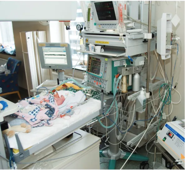
Cover: A newborn baby at the neonatal intensive care unit, the Queen Silvia children’s hospital, Göteborg, Sweden. The time-frequency plot in the background shows EEG power spectrum variations during sleep, and the EEG plot in the foreground shows a burst suppression pattern.

Photo: Yxell, Montage: Erik Lodin.

This research project was supported by a grant from the Margarethahemmet Foundation, the Swedish state under the ALF-agreement and the BIOPATTERN EU Network of Excellence, EU contract 508803.

Printed by Chalmers Reproservice Göteborg, Sweden 2009

I The brain requires a continuous supply of oxygen and nutrients, and even a short period of reduced oxygen supply can cause severe and lifelong consequences for the affected individual. The unborn baby is fairly robust, but there are of course limits also for these individuals. The most sensitive and most important organ is the brain. When the brain is deprived of oxygen, a process can start that ultimately may lead to the death of brain cells and irreparable brain damage. This process has two phases; one more or less immediate and one delayed. There is a window of time of up to 24 hours where action can be taken to prevent the delayed secondary damage. One recently clinically available technique is to reduce the metabolism and thereby stop the secondary damage in the brain by cooling the baby. It is important to be able to quickly diagnose hypoxic injuries and to follow the development of the processes in the brain. For this, the electroencephalogram (EEG) is an important tool. The EEG is a voltage signal that originates within the brain and that easily and non-invasively can be recorded at bedside. The signals are, however, highly complex and require special competence to interpret, a competence that typically is not available at the intensive care unit. This thesis addresses the problem of automatic classification of neonatal EEG and proposes methods that would be possible to use in bed-side monitoring equipment for neonatal intensive care units.

The thesis is a compilation of six papers. The first four deal with the segmentation of pathological signals (burst suppression) from post-asphyctic full term newborn babies. These studies investigate the use of various classification techniques, using both supervised and unsupervised learning. In paper V the scope is widened to include both classification of pathological activity versus activity found in healthy babies as well as application of the segmentation methods on the parts of the EEG signal that are found to be of the pathological type. The use of genetic algorithms for feature selection is also investigated. In paper VI the segmentation methods are applied on signals from pre-term babies to investigate the impact of a certain medication on the brain.

The results of this thesis demonstrate ways to improve the monitoring of the brain during intensive care of newborn babies. Hopefully it will someday be implemented in monitoring equipment and help to prevent permanent brain damage in post asphyctic babies.

Keywords: EEG, segmentation, classification, asphyxia, hypoxia, newborn, neonatal, cerebral

III This thesis is based on the work contained in the following papers:

Paper I Detection of burst and suppression in the EEG of post asphyctic newborns.

J. Löfhede, N. Löfgren, M. Thordstein, A. Flisberg, I. Kjellmer and K. Lindecrantz. 28th Annual International IEEE EMBS Conference, 2006, 2179-2182.

Paper II Classifying burst and suppression in the EEG of post asphyctic newborns using a support vector machine.

J. Löfhede, N. Löfgren, M. Thordstein, A. Flisberg, I. Kjellmer and K. Lindecrantz. 3rd International IEEE EMBS Conference on Neural Engineering, 2007, 630-633.

Paper III Classification of burst and suppression in the neonatal electroencephalogram.

J. Löfhede, N. Löfgren, M. Thordstein, A. Flisberg, I. Kjellmer and K. Lindecrantz. J. Neural Eng. 5, 2008, 402-410.

Paper IV Comparing a supervised and an unsupervised classification method for burst detection in neonatal EEG.

J. Löfhede, N. Löfgren, M. Thordstein, A. Flisberg, I. Kjellmer and K. Lindecrantz. 30th _{Annual International IEEE EMBS}

Conference, 2008, 3836-3839.

Paper V Automatic classification of background EEG activity in healthy and sick neonates.

J. Löfhede, M. Thordstein, N. Löfgren, A. Flisberg, M. Rosa-Zurera, I. Kjellmer and K. Lindecrantz. Submitted to the Journal of Neural Engineering.

Paper VI Does indomethacin for closure of patent ductus arteriosus affect cerebral function?

A. Flisberg, I. Kjellmer, J. Löfhede, N. Löfgren, M. Rosa-Zurera, K. Lindecrantz and M. Thordstein.

IV

Comparison of three methods for classifying burst and suppression in the EEG of post asphyctic newborns.

J. Löfhede, N. Löfgren, M. Thordstein, A. Flisberg, I. Kjellmer and K. Lindecrantz. 29th Annual International IEEE EMBS Conference, 2007, 5136-5139.

Application of a Very Simple Segmentation Algorithm to Burst Suppression Classification in Electroencephalogram Signals.

P. Damaschke and J. Löfhede. Submitted to Pattern Recognition.

V List of publications ... III 

Contents ... V 

Acknowledgements ... VII 

Notations and abbreviations ... IX 

Part I Introduction ... 1 

Chapter 1 Introduction ... 1 

1.1  Outline of the thesis ... 7 

Chapter 2 The brain ... 9 

2.1  Neurons ... 9 

2.2  Brain anatomy ... 11 

Chapter 3 The Electroencephalogram ... 15 

3.1  The 10-20 system ... 17 

3.2  Montages ... 17 

3.3  Types of EEG activity ... 18 

Chapter 4 Data and applications ... 23 

4.1  Data from healthy babies ... 23 

4.2  Data from post-asphyctic babies ... 24 

4.3  Data from preterm babies treated with indomethacin ... 25 

Chapter 5 Signal processing methods ... 29 

5.1  Filtering and pre-processing ... 29 

5.2  Artifact removal ... 30 

5.3  Features ... 30 

5.4  Feature characteristics and post-processing ... 36 

Chapter 6 Classification methods ... 39 

6.1  Classifier accuracy estimation ... 40 

6.2  Performance measures ... 41 

6.3  Maximum Likelihood Classification ... 42 

6.4  Fisher’s Linear Discriminant ... 43 

6.5  Artificial Neural Networks ... 44 

6.6  Support Vector Machines ... 49 

VI

Chapter 7 Feature selection ... 57 

7.1  Curse of dimensionality ... 58 

7.2  Exhaustive search ... 59 

7.3  Restricted search using genetic algorithms ... 59 

Chapter 8 Conclusions and future work ... 61 

References ... 65 

Part II Appended papers ... 69 

Summary of papers ... 71 

Paper I Detection of bursts in the EEG of post asphyctic newborns ... 75 

Paper II Classifying burst and suppression in the EEG of post asphyctic newborns using a support vector machine ... 87 

Paper III Classification of burst and suppression in the neonatal EEG .. 99 

Paper IV Comparing a Supervised and an Unsupervised Classification Method for Burst Detection in Neonatal EEG ... 119 

Paper V Automatic classification of background EEG activity in healthy and sick neonates ... 131 

Paper VI Does Indomethacin for Closure of Patent Ductus Arteriosus Affect Cerebral Function? ... 157 

VII The writing of this thesis and the work that it describes would not have been possible without our research group, a collection of people from the University of Borås and the Sahlgrenska University Hospital. First of all, I would like to thank my advisor Prof. Kaj Lindecrantz for his support and never ending enthusiasm. Also a big thank you to my co-supervisors: Dr Nils Löfgren, for his deep knowledge on EEG signal processing and practical advice on how to bend Matlab to ones will, and associate Prof. Magnus Thordstein for being a great golden standard and for coming up with new exciting research ideas. Thanks to Prof. em. Ingemar Kjellmer for the knowledge and inspiration, and Anders Flisberg for good collaboration and for all the interesting signals.

I would like to thank all the people that have been working with me or around me during these five years. The main part of this work has been carried out at the department of Signals and Systems at Chalmers and I would like to thank all the people there for making it such a great place to work, especially the people in the division of biomedical engineering and the crowd at floor 5. Thanks also to former colleague Johan Degerman who came up with the idea behind paper IV, and to Fernando Seoane for all the peptalks and discussions during these years.

For great assistance regarding the non-research related issues, I would like to thank Ann-Christine Lindbom, Agneta Kinnader and Madeleine Persson. Special thanks go my good friend Lars Börjesson for faithfully keeping track of the coffee breaks and for the assistance all the times that I have managed to mess up my computers in various ways.

I would also like to especially acknowledge my good friend Erik Lodin for the montage of the cover illustration.

Finally I would like to thank my fiancé Hanh for her never ending love and support, and for the new adventure that we are about to embark on. Smulan, thanks for being so patient and waiting for daddy to finish his thesis before entering this world.

IX

 variance

 mean

aEEG amplitude-integrated EEG ANN artificial neural network

AS active sleep

AUC area under the curve

AW active wake

BS burst-suppression BSR burst-suppression ratio CAR common average reference CFM cerebral function monitoring CNS central nervous system ECG electrocardiogram EEG electroencephalogram FLD Fisher’s linear discriminant

HMM hidden Markov model

ICU intensive care unit

ML maximum likelihood

NICU neonatal intensive care unit PCA principal component analysis pdf probability density function

QS quiet sleep

QW quiet wake

ROC receiver operating characteristic SEF spectral edge frequency

SVM support vector machine TA tracé alternant

Part

I

Introduction

1

Chapter

1

Introduction

The brain requires a continuous supply of oxygen and nutrients, and even a short period without them can cause lifelong effects. During delivery there is always a risk of insufficient circulation or blood gas exchange to the baby, something that may lead to asphyxia. This condition includes lack of oxygen, excess of carbon dioxide and a lowered pH value which can lead to permanent brain damage. Babies at risk are kept under close observation during delivery and afterwards at a neonatal intensive care unit (NICU), but it is hard to determine if the babies are recovering and if any brain damage has occurred. Parameters such as the heart rate, blood pressure and oxygen saturation are monitored regularly, but they are only measures of general conditions. If the function of the brain itself is to be monitored, the most direct way is to measure the electrical signals produced by the brain, the electroencephalogram (EEG).

The EEG is a voltage signal that is usually measured using metal electrodes placed on the scalp. It originates from electrical activity of the neuronal cells in the brain, and the EEG signal contains information about

2

the health status of a patient’s brain that can be interpreted by a clinical neurophysiologist. Earlier studies from our group have investigated how certain parameters calculated from the EEG signal can be used for detecting hypoxia (lack of oxygen) in the brain, and even for predicting the outcome after an hypoxic event [1].

In practice, most EEG recordings are evaluated through visual inspection of the unprocessed signal by a clinical neurophysiologist. Obviously, this methodology only allows for intermittent evaluations, and is not suitable for continuous bedside monitoring. Moreover, the expertise needed for this type of evaluation is typically not available at the NICU, and the patient cannot be transferred to a neurophysiologist for diagnosis. Even though methods for remote consultations have been developed [2], this methodology mainly allows for evaluation at distinct time instances and is not suitable for continuous bedside monitoring.

One attempt to simplify long-time monitoring of brain function that can be used for bedside monitoring is the amplitude-integrated EEG (aEEG). This method, in its most commonly used format, displays a filtered version of a two-channel EEG on a compressed time scale. It provides the clinician with a simple way to monitor the brain activity of a patient, and the compressed time scale gives a convenient view of several hours of recorded brain activity. However, this method has some severe limitations. For instance, interference and artifacts have in some cases been demonstrated to be hidden in the compressed signal and mistaken for brain activity, and there are also examples of missed seizure activity [3]. Because of these limitations, neurophysiologists argue that the unprocessed EEG signal has to be taken into consideration when interpreting the aEEG. This means that the staff at the NICU need to be able to interpret the signal at least to the level that they recognize artifacts and can distinguish between these and important brain activity. The staff has a lot of things to keep in mind, and adding complexity to their work would probably be problematic. Figure 1 shows an example of how the equipment surrounding a patient at a NICU may look.

To enable an improved continuous cerebral monitoring, we aim at developing methods for automatic classification and quantification of different types of activity in neonatal EEG. The input of the system should be a number of EEG channels and possibly additional parameters such as blood pressure and electrocardiogram (ECG) which normally are measured during these circumstances. The methods should be of a kind that can be implemented in a compact form suitable for use in a NICU environment, with easily interpreted parameters and alarms for threatening conditions of the brain. These parameters could serve as decision support for the clinician selecting the proper treatment or adjusting medication.

3 A functioning system of this kind will enable higher-quality care for high-risk neonates by providing clinicians with the possibility to continuously monitor the function of the brain itself, and not just the underlying support functions. Continuous monitoring will make it possible to follow the development of the status of the child over time, and enables the clinician to modify treatments and to follow the results in a real-time fashion, instead of having to rely on intermittent evaluations made by neurophysiologists.

A system like this could schematically consist of the following parts:  EEG amplification

 Digitization and storage

 Filtering of the EEG to reduce disturbances from surrounding devices

 Artifact rejection that marks epochs of questionable quality and excludes them from further processing

Figure 1: A newborn baby is treated after asphyxia during birth. The bed is cooled with circulating water to reduce further damage to the brain, and various parameters, e.g. aEEG (left screen), are monitored (Photo: Yxell).

4

 Activity classification algorithms that divide the data into different categories, pathological (indicative of disease) or normal. Both pathological and normal EEGs in neonates can be continuous or intermittent (alternating between two types of activity)

 Segment classification that quantifies the proportions of different types of activity in intermittent EEG

 Presentation of easily interpreted information to the attending staff

Figure 2 shows the system as a flowchart, all the way from the raw EEG signal to some easily interpreted parameter which can be displayed to the attending staff. The focus of this thesis is on feature generation, feature selection and classification of some different types of activity that can be found in neonatal EEG. The shaded boxes represent processes that are included in the thesis, but these processes are only active during development and are not to be included in the bedside equipment. Good EEG amplifiers and systems for storage and display of the acquired signal are available for clinical use [4] and are outside the scope of this thesis. The filtering that has been done was limited to simple highpass, lowpass and notchfilters implemented in Matlab, with especially the lowpass filters manually adapted to minimize the 50 Hz components that in some EEG recordings were dominant even after notch filtering.

The types of EEG under consideration consist of four behavioral states that are common in healthy full term neonates, one type that is typical for pre-term neonates (tracé discontinue) and burst suppression (BS) which is a type of activity sometimes found in very sick neonates. BS is intermittent activity characterized by a very low signal level (suppression) that is occasionally interrupted by sudden outbursts of higher signal levels (bursts). In the case that BS is detected, the automated analysis takes one step further and segments the pattern into burst and suppression, thus making it possible to calculate parameters such as the burst suppression ratio (BSR) and the suppression lengths which can be useful when arriving at a prognosis for a sick baby [5]. The tracé discontinue data was considered in a separate study where we applied the developed methods to the problem of investigating the possible presence of side-effects of a certain drug used to remedy a condition that sometimes can be found in preterm babies.

The methods that have been used include linear classifiers such as Fisher’s linear discriminant as well as nonlinear ones such as support vector machines (using a nonlinear RBF kernel) and neural networks. As inputs to the classifiers a number of features of the underlying EEG have been used. These features are parameters that are calculated from sliding windows that are moved along the signal, and enhance different

5 characteristics that are useful for classification. The classifiers can handle many features in combination, but just using all available features, or adding features at random, would not give the best classification since features that do not add useful information to the classifier will instead add noise. Therefore two methods for feature selection have been used: exhaustive search and restricted search using genetic algorithms. The exhaustive search simply tries all possible combinations of features on the classification problem, and the best combination can be selected. When the number of features grows this method quickly becomes too slow because the number of possible combinations grows very quickly. Restricted search using genetic algorithms on the other hand searches the space of possible combinations using methods inspired by natural selection and will usually find a solution close to the optimal one while trying much fewer combinations than the exhaustive search. However, the number of attempted combinations is still in the range of thousands, and because each attempt involves training and testing the classifier the genetic algorithm is too slow when used with the more advanced classifiers, and Fishers linear discriminator is preferred over them.

The results show that the developed methods can segment all the different intermittent EEG types that have been tested, and that burst suppression activity can be distinguished from normal EEG. If the developed methods were to be implemented as parts of a monitoring system they would provide improved insight into the brain function of babies at the NICU by being able to automatically detect if the baby is having BS and being able to automatically measure e.g. the suppression lengths. It can also classify the signal as normal, and indicate if the baby is sleeping quietly by detecting the presence of tracé alternant.

6

Figure 2: Monitoring system flowchart. The shaded boxes represent steps that are only included during development of the system, and that not need to be implemented in the bed-side equipment.

7

1.1

Outline

of

the

thesis

Part I contains an introduction to the area of neonatal monitoring and some background to the problems that have been worked on. Part I is divided into the following chapters:

Chapter 2 describes some relevant aspects of brain physiology. Neurons and synapses are described with emphasis on how they give rise to the potentials that are summed into the EEG signal. Then the major parts of the brain such as the cerebrum, cerebellum and brain stem are described to familiarize the reader with the basic structure of the brain.

Chapter 3 describes how the EEG signal is generated and how it can be measured. The electrode placement system and the different montages are described followed by an overview of some types of activity that can be found in the neonatal EEG.

Chapter 4 describes the data that has been available for experiments and used for training of the classifiers.

Chapter 5 describes the various signal processing methods that have been used in this project, with focus on the concept of generating feature signals intended to be used for automatic classification of the underlying signal.

Chapter 6 reviews the techniques for classification of signals that have been used throughout the project.

Chapter 7 describes why feature selection is necessary. Two methods for feature selection, exhaustive search and restricted search using genetic algorithms, are described.

Chapter 8 gives some conclusions and ideas for future work.

Part II contains the papers that are the foundation of the thesis. Summaries of these papers can be found in the beginning of Part II.

9

Chapter

2

The

brain

The chapter starts with a section dealing with the neuron, or nerve cell. This is the smallest unit in the construction of the wiring and logical system of the brain and of the entire nervous system. Then the anatomy of the brain is briefly described at a higher level, focusing on the cerebral cortex which is the main source of the EEG.

Most of the information in this chapter is based on [6].

2.1

Neurons

The neuron is the smallest functional unit in the brain and makes up a large part of the volume of the central nervous system (CNS). The rest of the volume consists of cells that support the neurons in various ways. A neuron has a very simple computational capability in itself, but by working together in vast neural networks they together form the complex system that is the human brain.

10

Figure 3: A neuron, with axon, dendrites and the cell body (soma).

The neuron generally has several different incoming connections, called dendrites, and one outgoing connection, called an axon (Figure 3). The axon of a neuron usually connects to dendrites of other neurons through synapses. A neuron works by summing the inputs from all dendrites before initiating an impulse along the axon, towards other neurons. The axons can be more than a meter in length (in the peripheral nervous system), and are often bundled into nerves. In the CNS, these aggregations are often called tracts.

Figure 4: Schematic representation of a synapse. An incoming action potential opens calcium channels in the synapse, and the calcium causes synaptic vesicles to release their contents of neurotransmitter molecules into the synaptic cleft. The molecules diffuse over to the post-synaptic cell, where a fraction of them bind to receptors in the cellular membrane. The receptors trigger in- or out-flux of ions and, when the membrane potential in the post-synaptic neuron reaches a certain threshold, a post-synaptic action potential is triggered. Afterwards, the neurotransmitters are released and may be recycled at the axon terminal.

Information flows through neurons as a depolarization of the cell membrane that causes ion channels in neighboring parts of the membrane to depolarize, and thus spread as a chain reaction that form an action potential that propagate along the axon and dendrites. When an action

11 potential reaches a synapse (Figure 4), it triggers a number of synaptic vesicles to release its content of chemical neurotransmitters into the synaptic cleft (the space between the pre-synaptic and the post-synaptic cell). The neurotransmitter molecules then attach themselves to receptors located in the cellular membrane on the receiving neuron on the other side of the synapse, triggering an inrush of ions that may start a new action potential and/or other alterations of the cell.

However, not all action potentials that reach a synapse trigger a new action potential in the receiving dendrite. The receiving neuron has thousands (or hundreds of thousands) of synapses. These synapses can be either excitatory, meaning that each synaptic activation increases the probability of the initiation of a post-synaptic action potential, or inhibitory, meaning that the synaptic activation decreases the probability of triggering an action potential. This increased or decreased probability of activation is transient; after a while the neurotransmitter molecules are removed from the synaptic cleft in preparation for receiving the next impulse. The neuron exhibits both temporal and spatial summation. Temporal summation means that many impulses in quick succession are summed and can together trigger an action potential. Spatial summation means that if many synapses are activated simultaneously their sum can trigger an action potential.

The spatial summation corresponds to summing a number of weighted inputs and using a threshold to decide if a binary output signal should be sent. The strength of a synaptic coupling can be enhanced by repeated activation, something that is believed to be the basis of learning. These characteristics are mimicked in the artificial neural network computational model described in section 6.5.

2.2

Brain

anatomy

The central nervous system (CNS) consists of the neurons described above, and of cells that support them. Examples of supporting cells are oligodendrocytes which wrap nerve fibers in fatty sheets that isolate them from one another and increase the signal propagation speed, or astrocytes which help to regulate the composition of the extracellular fluid by, for example, removing excessive neurotransmitter molecules that have leaked from the synapses.

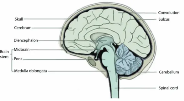
The CNS can be divided into the brain and the spinal cord (Figure 5). The spinal cord is the information highway which conducts sensory inputs from the body to the brain, and which also conducts commands from the brain to the various parts of the body but primarily to the muscles. The spinal cord does not contribute to the EEG and is therefore outside the scope of this text.

12

The brain can further be broken down into the cerebrum, the cerebellum and the brain stem. The brain controls the body through electrical impulses running along nerves from the brain via the spinal cord or the cranial nerves to different locations throughout the body, or through chemical messengers (hormones) that are created by various glands and spread to the body via the circulatory system.

2.2.1

The

cerebrum

and

the

cerebral

cortex

The largest part of the brain is called the cerebrum and it has a layered structure. The outer layer, the cerebral cortex, is about 1.5-4.0 mm thick and consists of nerve cells, which are brownish gray in color and therefore called gray matter. The cortex is convoluted, which gives it a large area, and is itself a layered structure with six layers, numbered 1-6 from the surface inward. The part of the cerebrum under the cortex is called white matter. It consists mainly of axons wrapped in myelin, a fatty substance that isolates the axons from each other and increases the signaling speed. The cerebral cortex is involved in most high-level functions such as perception, the generation of voluntary movements, reasoning, learning and memory. Different functions are mapped to different parts of the cortex. It can, for example, be shown that different touch sensors throughout the body are mapped to different parts of the cortex. Other parts of the cortex receive signals from the eyes, or the ears, or are responsible for planning movements. Various cortical areas are highly interconnected and higher functions like relating a visual impression to a remembered name, and then pronouncing the name involve many parts of the cerebral cortex.

13

2.2.2

The

cerebellum

The cerebellum is an important center for coordinating movements, ordered for example by conscious planning performed in the cerebrum, or regulating unconscious movements such as controlling posture and balance. The cerebellum receives information from various parts of the body, such as muscles, skin, eyes and the parts of the brain that are involved in control of movements.

2.2.3

The

brain

stem

The brain stem consists of the pons and the medulla oblongata. The brain stem contains all nerve fibers passing between the spinal cord, the cerebrum and the cerebellum, and most of the neuronal bodies of the cranial nerves. It also contains centers for vital functions such as respiration and circulation.

2.2.4

The

thalamus

The thalamus is a part of the diencephalon (Figure 5), which together with the cerebrum forms the forebrain. The thalamus is believed to translate incoming information and relay it to the appropriate parts of the cerebral cortex and therefore plays an important part of the generation of EEG signals.

15

Chapter

3

The

Electroencephalogram

The word ‘electroencephalogram’ (EEG) originally denoted the graphs showing the signals obtained by registering potential differences between electrodes placed on the scalp. Over the years, however, the term EEG has been used when referring to the signal itself, the technique to register the signal, or the printed graph. In this thesis EEG is used to denote the signal, unless otherwise stated.

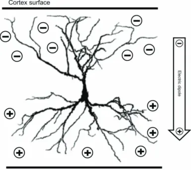
The potential differences between the electrodes are generally believed not to be caused by the action potentials that carry information between neurons, but rather by the postsynaptic potentials that appear in the synapses of the dendrites of the large pyramidal neurons [7]. These neurons are located in layers three and five of the cerebral cortex, but their dendrites stretch throughout several layers towards, and approximately orthogonal to, the cortical surface. The postsynaptic potentials are caused by the release of neurotransmitter substances into the synaptic clefts of the neurons, and each neuron can have tens of thousands of synapses. The postsynaptic potentials can be both excitatory and

16

inhibitory. The former type is associated with an extracellular surplus of negative ions while the latter is associated with a surplus of positive ions, giving them different electrical potential. There is a relative difference in the distribution of excitatory and inhibitory synapses between the part of the neuron that is close to the cortex surface and the deeper part which creates an electrical dipole pointed inward, as illustrated by Figure 6. For these signals to be large enough to make a measurable contribution to the electric field on the scalp, large areas of the cortex need to be synchronously active. This synchronicity is due to the fact that groups of neurons are simultaneously stimulated by impulses originating in the thalamus.

The electrodes used when registering EEG can be either metal plates, attached to the skin with the help of a conductive paste, or needle electrodes, stitched through the skin. When using electrodes placed on the exposed surface of the cortex, the recorded signal is called an electrocorticogram (ECoG). The signal levels are usually in the range of 20-100 V when measured at the scalp, but can be a few millivolts when measured invasively at the surface of the cortex.

The temporal resolution of the EEG is very good, and changes in the activity of the brain can be detected instantly. The spatial resolution is however bad, because signals from different sources are mixed through superposition. This means that the timing of EEG activity can be

Figure 6: A cortical pyramidal cell with net charges marked by + and -. A relatively larger amount of inhibitory synapses close to the cell body gives a surplus of positive ions, while a relatively larger number of excitatory synapses in the dendrites closer to the surface give a surplus of negative ions. The result is an electrical dipole pointed inwards.

17 determined very accurately, but it is more difficult to determine where in the brain the activity is taking place.

3.1

The 10‐20 system 

The electrodes are often placed according to the international 10-20 system [8] which defines a number of electrode locations by dividing the head into 10% and 20% intervals using the nasion and the inion as landmarks for the front to back direction and the preaurical points for the side to side direction (Figure 7), which defines 21 electrode positions. The first letter in the electrode name indicates which region it is placed over: F

for frontal lobe, C for the central line dividing the head in a rear and front half, P for parietal lobe, O for occipital lobe, and T for temporal lobe. Numbers in the electrode name are odd for the left hemisphere and even for the right, and increase with increased distance from the midline. A Z

refers to an electrode placed along the midline.

Figure 7: Landmarks and electrode locations of the 10-20 system (Figure from [9]).

3.2

Montages 

When measuring one voltage signal at least two electrodes are needed: an active electrode and a ground. However, in practice EEG signals are measured using differential amplifiers where the difference between two electrodes is amplified, and the ground electrode is separate. This is done because the EEG signals are very small, and interference from electrical appliances can cause large problems by making the potential of the patient vary in relation to the measuring equipment, and not involving the ground in the actual measurement decreases this problem. The ground electrode is still needed for connecting the amplifier ground to the patient ground; otherwise potential differences may arise that cause problems with

18

common-mode interference. It is also needed because of the small bias currents that enters the amplifier through the sensing electrode inputs, and has to return to the patient.

When measuring multiple channels, as is usually the case when measuring EEG, one of the two inputs from each of the differential amplifiers can be connected to a single reference electrode. All the channels then have the same reference when measured, but when viewing the signals the channels can be combined in different ways. The way the channels are combined when displayed is called the montage. Some common montages are listed below.

 The referential montage uses the designated reference electrode.

The location of the referential electrode varies, but it is usually placed somewhere along the midline of the head so that no emphasis is placed on any one of the hemispheres. Another alternative is “linked ears”, where electrodes on the ears are connected to each other and used as reference.

 The bipolar montage displays the difference between pairs of

usually adjacent electrodes.

 The common average reference (CAR) montage displays the

difference between the sensing electrode and the average of all channels.

Note that in the bipolar and CAR montages the reference input is mathematically eliminated when the difference of different electrodes is calculated.

In this work the common average reference montage has been used. An advantage of this montage is that interference occurring at all channels is cancelled by the subtraction of the average. Another advantage is that each displayed channel shows the local activity compared to the total activity of the brain, thus improving the spatial localization of the activity as compared to the bipolar montage where the displayed activity is the difference between two adjacent electrodes.

3.3

Types

of

EEG

activity

The EEG activity can be divided into different groups, of which some can be labeled normal and some are considered abnormal, or pathological

(indicative of disease).

However, normal is a very broad statement in the case of EEG. The signal picked up by EEG electrodes can have many different characteristics and still be labeled as normal, depending on for example sleep stage or age. Some frequency-based categories of EEG are described in Table 1. These designations originally arose because rhythmic activity within certain

19 frequency bands was found to have biological significance, or associated with certain regions of the scalp.

Most of the cerebral activity is traditionally thought to be found in the range 1-20 Hz, but recent research suggests that important information can be found in the extremely low frequencies that most EEG amplifiers filter away [10].

Name Frequency limits Location Properties

 (delta) 0.5 – 3.5 Hz Widespread Occur in infants and during deep sleep or anesthesia.

 (theta) 3.5 – 7.5 Hz Mainly in parietal and temporal lobes

Most prominent in small children and during drowsiness or sleep.  (alpha) 7.5 – 13 Hz Rear half of the

head Occur during awake and resting state, high amplitude when eyes closed. Mostly sinusoidal shape.  (beta) above 13 Hz Most common

in frontal and central regions

Often divided in two sub-bands, of which the higher frequencies appear during tension and intense activation of the CNS and the lower are attenuated during mental activity.

Table 1: Properties of some common EEG rhythms. The first four frequency bands are not overlapping and cover the whole EEG spectrum, even though the higher frequencies

of the  band are today usually named  rhythms.

The above-mentioned types of activity are “continuous” in the sense that they describe more or less rhythmic activity that goes on for some time, until they are changed by some change in mental state or sleep stage. Many of the types listed below are intermittent, meaning that one kind of activity is interrupted by sudden outbursts of other kinds of activity. In the seizure case, one type of activity (seizures) can also be superimposed on another (e.g. burst suppression).

Seizures (Figure 8) are the result of abnormal synchronization of groups of neurons and may or may not give rise to clinical symptoms (symptoms that are easily noticed in the clinic). The type of symptoms depends on which part of the brain that is affected. If it is a motor area of the brain, then the result can be wild and uncontrollable motion of the body. On the other hand, if it is a sensory area in the brain that is affected, the result may be that the person experiences e.g. visual flashing or unpleasant odors. There may also be sub-clinical seizures that do not cause any detectable symptoms, but are present in the EEG. Some newborn children

20

have seizures, the majority of which are sub-clinical. Even sub-clinical seizures may be harmful to the brain, implying that there is a need to detect and classify this type of activity so that children having seizures which are not apparent can be given the appropriate treatment.

Burst-suppression (BS, Figure 9) is one of several indicators of severe

pathology in the electroencephalogram (EEG) signal that may occur after brain damage, caused by e.g. asphyxia (insufficient oxygen and nutrient supply) around the time of birth [11, 12]. Certain characteristics of this pattern can provide clinicians with important information about the prognosis of the patient, and are thus important in the adjustment of the

Figure 8: One minute of seizure activity from an asphyctic baby. The seizure is concentrated to the left part of the rear of the brain, and combined with a BS pattern with a burst around 16:05:17. The high frequency noise in P4 and T6 is probably due to that the baby was lying with the right side down. The ECG signal (bottom graph) is included for comparison.

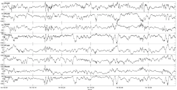
Figure 9: One minute of burst suppression from an asphyctic baby, with two visually classified bursts marked with shading.

21 treatment. Examples of important characteristics of the BS pattern are the length of the burst and suppression intervals, the percentage of suppression activity in a recording, and the spectral contents of the bursts [5, 10, 13].

Tracé discontinue (Figure 10) is visually somewhat similar to burst

suppression, but is normal in premature babies [14]. Periods with low amplitude or inactivity alternate with activity with higher amplitude and mixed frequency content. This type of activity dominates most recordings from premature babies, without depending on state, but is most marked during quiet sleep. The interburst durations decrease as the infant matures and the properties of the interburst activity change, and the activity during quiet sleep evolves into tracé alternant.

Tracé alternant (Figure 11) is a pattern with alternating active and less

active periods that is seen in healthy full-term children during quiet sleep [14]. Instead of the suppression or inactivity that is seen in BS or tracé

discontinue there are low activity periods that contain low frequency

activity. The low activity is interrupted by random high activity periods containing transients with higher frequency and amplitude. Tracé

alternant usually emerges 34-36 weeks after gestation, but there is a

significant overlap between tracé discontinue and tracé alternant before the baby reaches full term.

22

Figure 8 - Figure 11 were produced using a notch filter at 50 Hz, a low-pass filter at 70 Hz and a linear detrend filter. Often a high-low-pass filter is used to remove slow baseline fluctuations, but that would change the appearance of the low-frequency components in e.g. many of the bursts.

Figure 11: One minute of tracé alternant recorded from a healthy baby during quiet sleep.

23

Chapter

4

Data

and

applications

This section describes the three categories of data that have been used in the project. The data were collected at the Queen Silvia Children’s Hospital, which is a part of the Sahlgrenska University Hospital in Göteborg. Details regarding the collection of the EEG signals can be found in the respective paper.

4.1

Data

from

healthy

babies

The common denominator for all papers included in the thesis is solving problems that are of interest when building a monitoring device for the NICU. The most important function of such a monitor is to be able to distinguish activity recorded from a healthy baby with no brain-related problem from activity from a sick baby. Therefore EEG signals were collected from 20 healthy full term newborn babies that had uneventful deliveries. Data were collected during a few hours so that the four behavioural states active awake (AW), quiet awake (QW), active sleep (AS) and quiet sleep (QS) [15] could be included in most of the

24

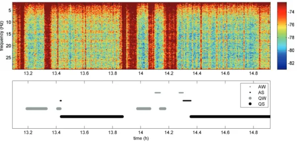
recordings. These data were divided into the four states based on the observations made by the technician performing the recording and on the classification made by an experienced electroencephalographer. For quiet sleep, EEG of the tracé alternant type was chosen. Figure 12 shows a time-frequency plot of one of the recordings. The most prominent features of this plot are the red high power strips, but these are not caused by the actual EEG signal but are mostly due to artefacts produced by the muscles on the baby’s scalp during crying.

4.2

Data

from

post

‐

asphyctic

babies

The second group of babies consists of six full-term neonates that were suffering the after-effects of asphyxia during birth. This condition includes lack of oxygen, leading to a build-up of carbon dioxide and a lowered pH value in the blood, and can, among other things, lead to brain damage. These babies all exhibited a severe burst suppression pattern in their EEG. Continuous EEG recordings, of between 6 and 40 minutes in length, were made for each of the six babies. The recordings were then visually classified by an electroencephalographer. The length of each recording was chosen to include at least 10 bursts, and all artefacts were visually identified and marked for later exclusion from the analysis. The total amount of data in this category was 77 minutes.

For evaluation of the BS-related methods in a setting as close as possible to the clinical one, a 32 hour recording from one of the six babies was used. The baby had to be resuscitated after birth and was then intubated and put on a ventilator. The EEG recording was started six hours after birth and continued for 32 hours with a short break around 18 hours after start. The ventilator frequency was set to 40/min (0.7 Hz) initially and was

Figure 12: Time-frequency plot of 2h of EEG from a healthy newborn baby, with the behavioural states marked. The unmarked high-power red strips are mainly episodes of crying, with the high power mainly due to muscle artefacts from the scalp.

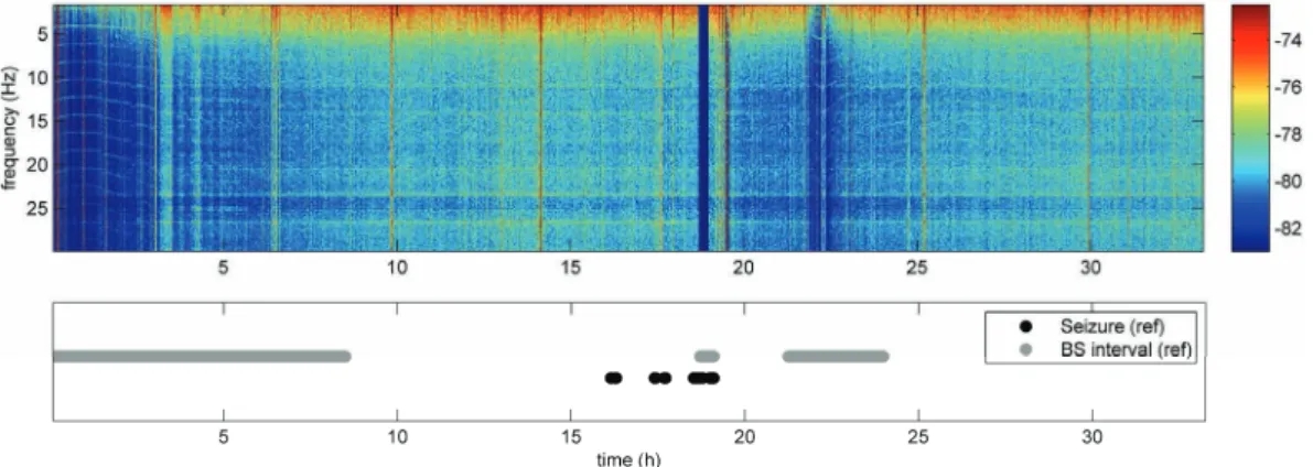
25 changed to 30/min (0.5 Hz) 16 hours after start. At 18 hours after the start of the recording, a dose of Phenobarbital was given to treat seizure activity. The baby was later diagnosed with cerebral palsy. Figure 13 shows a time-frequency plot of this recording, where two long BS episodes can be seen as depressions in the mean power of the signal. Some seizure episodes are also marked, but are too short compared to the scale of the figure to be visible in the plot.

4.3

Data

from

preterm

babies

treated

with

indomethacin

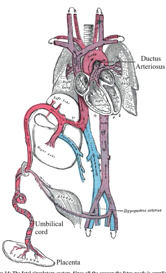
While the two preceding groups of babies all where full term, the babies in the final group were born prematurely, between 25-33 weeks of gestation, and were displaying the intermittent tracé discontinue pattern that is normal for this patient group. These babies were all diagnosed with a clinically persistent ductus arteriosus, meaning that the shunt that allows blood in the unborn fetus to by-pass the lungs did not close, which it normally does autonomously shortly after birth (Figure 14 and Figure 15). This imposes circulatory disturbances that increase the risk of brain damage. To induce closure of the ductus arteriosus the drug indomethacin can be used. There have however been concerns raised to whether this may have a negative effect on the brain because of the drug’s vasoconstricting properties, i.e. it tends to make the blood vessels temporarily contract and thereby reduce the blood flow. To examine this, seven premature neonates with clinically significant persistent ductus

arteriosus were recruited. EEG signals were recorded before, during and

after an intravenous infusion of indomethacin over 20 minutes, and the effect on the brain was estimated by automatic segmentation of the EEG and measuring the length of all low activity periods.

Figure 13: Time-frequency plot of 32h of EEG from a post-asphyctic baby with episodes of BS and seizures marked. The dark blue strip around 18h is a gap in the recording.

26

Figure 14: The fetal circulatory system. Since all the oxygen the fetus needs is supplied by the mother via the placenta and the umbilical cord, the lungs are not vital for gas exchange before birth, and the blood is partly allowed to bypass them through the ductus arteriosus (figure from [16]).

27

Figure 15: Schematic of the circulatory system in adults and fetuses. The foramen ovale is a hole that allows passage of blood from the right to the left atria.

29

Chapter

5

Signal

processing

methods

In this chapter the signal processing methods used in the project are described. All methods mentioned are based on sampled, discrete signals as opposed to analog continuous signals. Many of the measures used to describe these signals are statistical, and related to the shape of the distribution of the signal. Others estimate the frequency contents, the power of the signal, or the information content. These measures are here termed features, because this term is common in classification literature, and because the measures are meant to describe different characteristics, or features, of the underlying EEG signal.

5.1

Filtering

and

pre

‐

processing

The amplitude of the EEG is very low when measured from the scalp, in the range of tens of microvolts, making it very sensitive to interference from surrounding electrical fields created by common electrical appliances. These interferences are typically common mode, meaning that they appear on all leads simultaneously. Using the common average

30

reference (CAR) montage described in section 3.1.2 helps to suppress this interference because the mean of all channels is subtracted.

Usually 50 Hz noise caused by interference from surrounding electrical equipment is present in the EEG to some extent, and therefore a notch filter at this frequency has been used in all cases. In some cases when the EEG has been extremely suppressed, the 50 Hz was still dominant after notch filtering and a low-pass filter with cut-off frequency at 44 Hz with zeros that coincided with the 50 Hz peak was used. In other cases cut-off frequencies of 20 and 70 Hz have been used, depending on the application.

The data was also high-pass filtered. It has been shown that important information in neonatal EEG is present in the very lowest frequencies [10, 13], but because of interference sources, some of the sick babies were e.g. ventilated at a frequency of 0.3-0.7 Hz, a high-pass filter was used. In some cases a cut-off frequency of 0.5 Hz was enough, while others required a cut-off at 1.6 Hz. If information from these low frequencies is needed in a monitoring device, once the classification process is finished it would be possible to go back to the raw EEG signal and apply a different processing on the segments of interest using the classification results.

In one of the BS patients (patient 3, Paper II and onwards), an LMS (least mean square) adaptive filter [17] with a separate ECG channel as reference was used to suppress ECG interference in the EEG signal.

5.2

Artifact

removal

For the BS segmentation process, periods that were manually identified as artifacts were removed from the set after the feature extraction step, and were not included in the training or evaluation of the classification methods. The reason for including them in the feature extraction is that cutting a signal may introduce sudden steps in the resulting signal when the remaining parts are merged. These steps are of a high-frequency nature and would influence many of the features described in section 5.3. Therefore all relevant parameters should be extracted before any cutting of the signal is performed.

For the classification into different states, no artifacts were removed. Because much longer windows were used, most artifacts were drowned in the real EEG activity and were therefore judged to be negligible.

5.3

Features

The EEG signal is not random, but it is complex enough to be described in stochastic terms as a random process. Medical EEG specialists mainly use visual inspection of the waveforms in the time domain to classify the

31 activity. However, when building a signal processing system for classifying signals, well-defined measurable features that can be implemented using mathematical functions are needed. Examples of features are the total power of a signal or the distribution of the power with respect to frequency. These two features measure two different properties of the underlying signal and can be independent, because two signals with the same total power could have totally different power spectra.

All the features used here are extracted from sliding windows, because it is not possible to calculate spectra or statistical measures on single samples. A sliding window is an interval of the signal, for example one second long. With a sampling frequency of 200 Hz, 200 samples will fall into this window, giving a statistical basis for calculating different parameters. Each parameter yields one value for each window. When the parameters have been calculated for a window, it is moved a certain distance along the signal, for example 0.25 s, and the parameters are calculated for the samples that now are inside the window. Moving the window a distance that is smaller than the width of the window results in a certain overlap, in this example 0.75 s. The operation also results in a reduction in effective sampling frequency, from the original 200 Hz to 4 Hz, since now four samples are used to describe one second of the signal instead of the original 200. This reduces the temporal resolution for detection, but since the quality of the parameters calculated from the data in the window generally increases with increasing number of samples, this results in a trade-off between time resolution and feature estimation accuracy.

When using sliding windows, the length of the window and the distance it is moved in each step have to be decided. If the window is too short, there is too little information in each window to calculate a spectrum of sufficient resolution, or to calculate statistical parameters with high enough reliability. If it is too long, short periods of activity in the EEG could be drowned by other activity surrounding it. In the case of burst-suppression, a window length of one second was chosen, determined by the fact that the shortest bursts in the available material were one second long, and in the state classification case metafeatures, i.e. features of the features were used, with a window length of 30 s (see section 5.4.1). The step length that the window is moved is not as critical as the window length. A short step length results in a large overlap between consecutive windows, and produces smooth output signals. A longer step length reduces the effective sample rate of the output signal, thus reducing the computation time for the following processing steps.

32

5.3.1

Spectral

Edge

Frequency

The spectral edge frequency (SEF) [18] of a signal is the frequency under which a certain percentage (e.g. 95%) of the power resides. This gives a measure of the shape of the frequency distribution, because for an EEG signal there will always be power in the low frequency range. SEF is a common measure used in EEG monitoring, and has for example been used for estimating the depth of general anesthesia, when a patient is made unconscious for surgery.

5.3.2

Three

‐

Hz

power

This feature measures the power in a 1 Hz wide band centered around 3 Hz, and was inspired by earlier work [19] in which it was used for detecting BS under anesthesia. BS is often characterized by low frequency content [10, 13] making low frequency features simple and natural choices.

5.3.3

Median

The median [20] is the number that divides a distribution in two equal parts. It can be found by sorting the numbers and taking the middle one. For a normal distribution the median is equal to the mean, but for e.g. the exponential distribution it is not. When estimating parameters from a limited set of samples, the median is less sensitive to outliers (extreme values) than the mean.

The behavior of the median for BS segmentation depends on the filtering. The median will act as a low-pass filter with frequency characteristics depending on the window length, and probably capture the low frequency part of the bursts. However, if the signal is high-pass filtered (by processing or by bad electrode coupling) the bursts would be transformed into zero-mean signals, and the median would not be usable as a feature.

5.3.4

Shannon

Entropy

The Shannon Entropy [21] is a measure of uncertainty of a random variable, or in other words the information content. It is estimated by defining a set of bins that divide the amplitude range into disjoint intervals I1,..,IU and then estimating the probabilities p(I1)… p(IU) by

counting the number of samples which fall into each bin.



In the present implementation, 20 bins distributed between +/- were used, where  is the standard deviation of the EEG amplitude in each window of the signal.

33 When applied on a BS signal the entropy decreases during the burst intervals. This is due to the fact that the suppression activity is mainly just noise, having high entropy, while the bursts are comparatively more ordered with a combination of low and high frequencies.

5.3.5

Zero

Crossings

The rate of zero crossings [18] was investigated as a way to measure frequency contents of a signal in the era before inexpensive computer chips, and it is implemented by measuring how often the signal crosses the zero level. This is not simply related to the frequency of the signal, since a high-frequency component superposed on a low-frequency component may not cross the zero level very often.

5.3.6

Variance

The variance [22] is defined by









where X is a random variable and E(X) is the expected value of X. The variance is also denoted σ2_{, where σ is the standard deviation of the}

probability density function of X. The standard deviation is a measure of the degree of spreading of the distribution around the expected value. In the time domain, a large standard deviation would imply that the signal contains a large fraction of samples with amplitudes that are far away from the mean, while a low standard deviation implies that the samples are mostly close to the mean.

Numerically, the variance is estimated as the mean of the squared difference between each sample and the sample mean:





where μ is the sample mean. Often the signal is zero-mean, which makes the variance equal to the mean power of the signal (the mean of the squared sample values).

Since burst periods above all are characterized by having higher power than suppression periods, the variance is a natural starting point for BS segmentation.

5.3.7

Skewness

The skewness [22] of a distribution is defined by









34

and is a measure of how symmetric the distribution is. In the time domain for a zero-mean distribution, a high skewness value would imply that most of the samples with amplitude deviating from the mean are positive.

Numerically, the skewness is estimated as the cube of the sample mean of each sample’s deviation from the sample mean, normalized by the cube of the standard deviation:

3 1 3 1 ) ] [ ( 1 ) (  



The skewness was mainly used as a meta-feature (section 5.4.1) applied on the other feature signals. For example, the skewness of the residual energy variance was included when classifying BS from other types of EEG (Paper V). The skewness was also considered for BS segmentation in Paper I.

5.3.8

Kurtosis

The kurtosis [22] of a distribution is defined by









and is a measure of how “peaky” a distribution is. Higher kurtosis means that more of the variance is due to infrequent extreme deviations.

Numerically, the kurtosis is estimated as the mean of each sample’s deviation from the sample mean raised to the power of four, normalized by the standard deviation raised to the power of four:

4 1 4 2 ) ] [ ( 1 ) (  



The kurtosis was mainly used in the same way as the skewness, as a meta-feature. For example, the kurtosis of the spectral roll-off was used for classifying BS from other types of EEG (paper V). The skewness was also considered for BS segmentation in Paper I.

5.3.9

Spectral

centroid

The spectral centroid [23] is commonly used for characterizing sound. It is the “centre of mass” of the spectrum, calculated as a weighted mean of the frequencies in the signal with their magnitudes as weights:

 

 





35 where X is the Fourier transform of the signal and K is the number of points in the estimated spectrum. Since the value of K is not physical frequency but depends on the sampling frequency and the number of points used for estimating the spectrum, the value of c will have to be scaled to get the value of the centroid in hertz. When used as a feature, the actual value is usually not of interest, but rather the distribution of the feature for the different classes that are to be classified.

5.3.10

Residual

energy

variance

The residual energy variance is a measure of how accurately the signal can be predicted by a filter of a given order, and is related to the entropy of the signal. The feature was implemented by finding the eight coefficients of the linear prediction filter that minimized the prediction error in the least squares sense. The order of the filter was determined by estimating the maximum number of peaks in a typical EEG signal. The residual was calculated as the output of filtering the signal through the prediction filter, and then the variance of the residual was calculated.

5.3.11

Spectral

flux

The spectral flux [24] measures the change in the spectrum between consecutive windows using the squared Euclidian distance (2-norm) between the spectra:

 

 







where X1 and X2 are spectra for two consecutive windows of the signal,

and K is the number of points in the estimated spectrum.

5.3.12

Delta

flux

The delta flux feature measures the rate of change in the signal by taking the square of the Euclidian distance between consecutive windows of the signal in the time domain:

   







where x1 and x2 are the signals in the time domain and N is the number of

samples in the window.

5.3.13

Spectral

flatness

The spectral flatness [23] is a measure of how flat the spectrum is. A high spectral flatness indicates that the spectrum has a similar amount of power in all bands – like white noise. A low spectral flatness indicates a spiky spectrum, like a mixture of sinusoids.

36

The spectral flatness is calculated by dividing the geometric mean of the power spectrum with the arithmetic mean:

 

 





where X is the Fourier transform of the signal and K is the number of points in the estimated spectrum.

5.3.14

Spectral

roll

‐

off

The spectral roll-off is based on the same principle as SEF95 and measures how wide the spectral distribution is, but uses the frequency for 85 % of the energy instead of 95. This feature is common in sound processing [25], hence the different name.

5.3.15

Cepstrum

‐

based

coefficients

The cepstrum is defined as the inverse Fourier transform of the logarithm of a spectrum and contains information about the rate of change in the different frequency bands. In the current implementation, ten triangular overlapping windows were applied on the spectrum before transformation, resulting in ten coefficients that each is related to a frequency band.

5.4

Feature

characteristics

and

post

‐

processing

After feature generation some steps need to be taken to prepare the feature signal for the classification algorithms. Some of these steps, such as the normalization procedure, were chosen to reduce the differences between recordings from different patients that were found to be a problem when segmenting BS signals (5.4.2). Others, such as the channel combination and feature smoothing, were chosen based on prior knowledge of the expected characteristics of the BS activity.

5.4.1

Meta

‐

features

For the state classifier (paper V), the features were summarized by applying the four statistical measures mean, variance, skewness and kurtosis on the feature signals from each 30 s non-overlapping epoch in the data, resulting in 88 features based on the original 22. This was done because sleep-stages and BS go on for some time, at least a couple of minutes, while e.g. a single burst can be as short as one second. These measures describe different properties of the feature signals distributions. For example, the mean and the variance are measures of where the distribution is located and how wide it is, while skewness and kurtosis measure its shape. These measures are in this paper called metafeatures, because they are features of the features of the EEG.