Improving Stability and Convergence for Adaptive Radial Basis Function Neural Networks Algorithm. (On-Line Harmonics Estimation Application)

Contents list available at IJRED website

Int. Journal of Renewable Energy Development (IJRED)

Improving Stability and Convergence for Adaptive Radial Basis

Function Neural Networks Algorithm

(On-Line Harmonics Estimation Application)

Eyad K. Almaita

and

Jumana Al Shawawreh

†_{Dept. of Electrical Power and Mechatronics Engineering, Tafila Technical University, Jordan}

ABSTRACT. In this paper, an adaptive Radial Basis Function Neural Networks (RBFNN) algorithm is used to estimate the fundamental and harmonic components of nonlinear load current. The performance of the adaptive RBFNN is evaluated based on the difference between the original signal and the constructed signal (the summation between fundamental and harmonic components). Also, an extensive investigation is carried out to propose a systematic and optimal selection of the Adaptive RBFNN parameters. These parameters will ensure fast and stable convergence and minimum estimation error. The results show an improving for fundamental and harmonics estimation comparing to the conventional RBFNN. Also, the results show how to control the computational steps and how they are related to the estimation error. The methodology used in this paper facilitates the development and design of signal processing and control systems.

Keywords: Energy efficiency, Power quality, Radial basis function, neural networks, adaptive, harmonic.

Article History: Received Dec 15, 2016; Received in revised form Feb 2nd _{2017; Accepted February 13}rd _{2017; Available online}

How to Cite This Article: Almaita, E.K and Shawawreh J.Al (2017) Improving Stability and Convergence for Adaptive Radial Basis Function Neural Networks Algorithm (On-Line Harmonics Estimation Application). International Journal of Renewable Energy Develeopment, 6(1), 9-17.

http://dx.doi.org/10.14710/ijred.6.1.9-17

1. Introduction

Recently, power quality has become a major concern for modern power systems. One of the main power quality issues is the harmonic distortion in power systems. The excessive presence in harmonics in power system can cause many problems such as: malfunctioning of circuit breakers and relays, overheating of conductors and motors, insulation degradation, and communication interference (Eyad Almaita, 2016; Izhar, Hadzer, Masri, & Idris, 2003; Rahmani, Hamadi, & Al-Haddad, 2009; Sumaryadi, Gumilang, & Susilo, 2009).

Different approaches have been used for harmonics mitigation in power systems. Active Power filters (APFs) are considered an effective means to reduce harmonics to acceptable levels. Any APF is consist of two main parts: (i) Control part that measures the distorted signal (voltage or current) then decomposed the measured signal into fundamental component and other harmonic components based on on-line harmonic estimation algorithm. (ii) Power part consists of power electronics

*Corresponding author: [email protected]

module to compensate for all harmonic distortions (Akagi, Watanabe, & Aredes, 2007). On-line harmonic estimation algorithms have been extensively studied. They can be classified into three main classes; (i) time domain algorithms, (ii) frequency domain algorithms, and (iii) artificial intelligent algorithms (Akagi, 1996; Rahmani et al., 2009; Wang, Wong, & Member, 2015; Yasmeena & Das, 2016; Zhang, Li, & Wang, 2010). Time domain algorithms always have to compromise between the phase delay and the attenuation, also, oscillations is always can be caused by fast transition time (Zhang et al., 2010). On the hand, frequency domain algorithms need high computations and considered not real-time filters (Zhang et al., 2010). The artificial intelligent (neural networks) algorithms have been successfully tested to overcome the disadvantages of the time and frequency domain filters. The three main techniques used in neural networks algorithms are (i) adaptive linear neuron (ADALINE), (ii) back propagation (BP), and (iii) radial basis function neural networks (RBFNN). The ADALINE is used as online harmonics identifier and its performance depends on the number of harmonics

included in its structure. The convergence of the ADALINE slows as the number of harmonics included increases because the ADALINE can only approximate linear functions (Chang, Chen, & Teng, 2010; Zouidi, Fnaiech, AL-Haddad, & Rahmani, 2008). On the other hand, The BPNN is more capable and can approximate linear and nonlinear function. It uses offline supervised training to identify selected harmonics. The long training time required in BPNN and the chance of falling into local minima is always present (Haykin, 1999; Kasabov, 1996). The RBFNN has several advantages over ADALINE and BPNN; capable of approximating highly nonlinear functions, its structural nature facilitate the training process because the training can be done in a sequential manner, and the use of local approximation can give better generalization capabilities (Haykin, 1999; Kasabov, 1996). Several schemes for RBFNN have been used; some of these schemes have large number of hidden neurons and still uses training algorithm similar to that of BPNN (Chang et al., 2010). Other schemes gets better results and with small number of hidden neurons using direct inversion matrix as training algorithm (E Almaita & Asumadu, 2011a, 2011b). An adaptive version of RBFNN has been introduced in ( Almaita, 2012). In this adaptive version the parameters of RBFNN can be modified after the deployment without the need of re-training the RBFNN. This gives an additional strength to the RBFNN. The main problem of this adaptive version is the learning rate, which needs to be selected very carefully to ensure the convergence and stability of the system.

In this paper, which is an extension to the works in (Almaita, 2012; Almaita & Asumadu, 2011a, 2011b), a systematic approach is introduced to select the parameters of the adaptive RBFNN algorithm. This approach will ensure the stability and will also minimize the estimation error. Also, the adaptive RBFNN will be used to estimate the fundamental and harmonic contents in current signal of non-linear load.

2. Conventional RBFNN

2.1 Structure of RBFNN

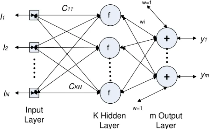
The RBFNN structure consists of three main different layers as shown in Fig. 1; one input layer (source nodes with inputs I1, I2,.., IN), one hidden layer has

K neurons, and one output layer (with outputs y1, y2,.., ym).

The input-output mapping consists of two different transformations; nonlinear transformation from the input layer to the hidden layer and linear transformation from hidden to the output layer. The connections between the input and hidden layers are called centers and the connections between the hidden and output layers are called weights (Almaita & Asumadu, 2011a, 2011b).

The most common radial basis function used in RBFNN is given by

i=1,2,…,K (1)

This is a Gaussian basis function with φi as the

output of the ith_{hidden neoron , x is the input vector data}

sample (I1, I2,…,IN) (could be training, actual, or test data),

ci is centers vector of the ith hidden neuron (ci1,ci2,.., ciN),

σi is the normalization factor, and (x-ci)T(x-ci) is the

square of the vector (x-ci) (Almaita & Asumadu, 2011a,

2011b). The ith _{output node yi is a linear weighted}

summation of the outputs of the hidden layer and is given by

𝑦𝑖= 𝑤𝑖𝑇∅(𝑥), i=1, 2,…., m (2)

where wiis the weight vector of the output node and Ф(x)

is the vector of the outputs from the hidden layer (augmented with an additional bias which assumes a value of 1).

2.2 Training Algorithm of RBFNN

The block diagram shown in Fig. 2 illustrates one of the RBFNN training processes called hybrid learning

process (Moody & Darken, 1989; Yousef & Hindi, 2005). The hybrid learning process has two different stages; (i) finding suitable locations for the radial basis functions centers of the hidden neurons (Moody & Darken, 1989; Yousef & Hindi, 2005) and (ii) finding the weights between the hidden and output layers. In the first stage the K-means (Moody & Darken, 1989; Yousef & Hindi, 2005) clustering algorithm is used to locate the centers in the input data space regions where a significant data are present (shown as I in Fig. 2). In the second stage (shown as II in Fig. 2) the weights between the hidden and the output layers are found by linear matrix inversion algorithm based on the least-square solution, which minimizes the sum-squared error function (Yousef & Hindi, 2005).

Figure 1 Structure of Conventional RBFNN Network f f f

+

+

 



 



Figure 2 Block Diagram for the RBFNN Hybrid Learning Process

The weights matrix w is given by

D A

w 1T ₍₃₎

where D is the desired output vector for l training data samples set and given by

(4)

where d(xj) describes the output vector corresponding to

the jth_{training data samples vector (xj).}  _{is a matrix}

where each element φi(xj), is a scalar value and

represents the output of the ith _{hidden neuron for the j}th

training data samples vector (xj).

The  matrix for l training data samples is given by

(5)

A-1_{, the variance matrix and given by}





1 



_

_

_

A

(6) One of the advantages of this method compare to other training algorithms is that it does not need iterations in the training phase; what it needs is the matrix inversion shown in Eq (6), which needs negligible time to be calculated.

3. Adaptive RBFNN

One of the major disadvantages of the feed forward neural networks (BPNN and conventional RBFNN) techniques is that; the obtained parameters do not changed once the training process is completed. In the presence of the noise, these fixed parameters can degrade the performance of the neural networks. The main objective of the adaptive RBFNN algorithm is to enhance

the reliability of the conventional RBFNN after embedding the network in the system. This can be achieved by introducing an adaptive algorithm for RBFNN structure that allows the change of the weights of RBFNN after the training process is completed. As shown in II, the RBFNN adjustable parameters that will affect the output are the centers and the weights. This algorithm assumes that the noise present in the system can be mitigated only by adjusting the weights between the hidden and the output layers, without the need of adjusting the values of the centers between the input and hidden layers.

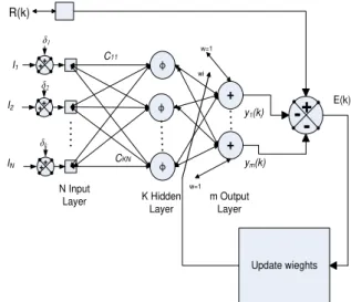
Figure 3 shows the general structure of the adaptive RBFNN algorithm. It has the same conventional RBFNN structure regarding input layer, hidden layer, and output layer. But it has two extra components; (i) Summation component, which is located after the outputs of the RBFNN. The goal of this component is to calculate the error signal between the estimated outputs y and the reference (actual) signal (R). (ii) Weights updating component. The goal of this component is to adjust the weights in order to reduce the error signal. In the absence of the noise δ(k) in the input side, the summation of the outputs of the RBFNN model is equal to the reference signal R(k).

Figure 3 General Structure of Adaptive Conventional RBFNN Network

In this case the error E(k) equal to zero and no change in the RBFNN weights.

𝐸(𝑘) = 𝑅(𝑘) − {𝑦1(𝑘) + 𝑦2(𝑘) + ⋯ + 𝑦𝑚(𝑘)} (7)

In the presence of noise in the input side, the jth output node of the RBFNN will be affected by this noise as 𝑦𝑗(𝑘) = 𝑦𝑜𝑗(𝑘) + 𝛿𝑗(𝑘) (8)

where 𝑦_𝑜𝑗(𝑘) is the jth output node without noise and 𝛿𝑗(𝑘) is the added noise error to the jth output node.

φ φ φ + + I1 N Input Layer K Hidden Layer m Output Layer y1(k) C11 wi w=1 w=1 I2 IN CKN ym(k)

-+

I II                      ) ( . ) ( . ) ( ) ( l x d j x d x d x d D 2 1                   ) ( ... ) ( ) ( . . ... . . . . ) ( ... ) ( ) ( ) ( .... ) ( ) ( l x K l x l x x K x x x K x x          2 1 2 2 2 2 1 1 1 2 1 1

In this case the error E(k) is not equal to zero.

In order to mitigate the effect of the noise in the performance of the RBFNN, the error E(k) is used to update the weights vectors based on the least-mean- square-error algorithm (Moody & Darken, 1989) as:

𝑤1𝑛𝑒𝑤= 𝑤1𝑜𝑙𝑑+ µ1∅(𝑘)𝐸(𝑘) (9)

⋮

𝑤𝑚𝑛𝑒𝑤= 𝑤𝑚𝑜𝑙𝑑+ µ𝑚∅(𝑘)𝐸(𝑘) (10)

where µj is the regulation factor for the jth output node.

The weights updating will continue until the error E(k) become zero again. The above algorithm has several advantages including the following:

 It has a fast convergence time because it adjusts only the weights between the hidden and output layers, which is a linear relationship. Therefore, fast convergence can be achieved.

 The updating process could be initiated based on threshold value for E(k) (different from zero), which gives the flexibility to the algorithm and saves excessive computations. This algorithm has greater capabilities compare to the popular neural linear adaptive algorithm (ADALINE) because the RBFNN structure can be used to realize linear and nonlinear functions.

4. Methodology

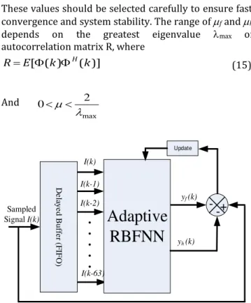
Figure 4 shows the inputs and outputs signals for the adaptive RBFNN used in this paper. The input signal is sampled at constant rate and passed through first-input-first-output (FIFO) buffer to create a delayed vector with length 64, represent a half cycle of the signal, which match the length of the input vector of RBFNN. The adaptive RBFNN used in this paper has two outputs; one of them is to estimate the fundamental component (yf)

and the other is to estimate the harmonic components (yh), these outputs are calculated as follows:

(11) (12) where Wf, Wh, is the weight vector of the fundamental

and harmonic components output , respectively and Ф(x) is the vector of the outputs from the hidden layer. The accurate online estimation of the fundamental and harmonic components depends on continuous updating of the weight vectors of fundamental and harmonic components Wf, Wh,

respectively, as illustrated in III. Updating the weight vectors depends on the values of regulation factors f

and h as follows:

(13) (14) These values should be selected carefully to ensure fast convergence and system stability. The range of f and h

depends on the greatest eigenvalue max of autocorrelation matrix R, where

(15) And

Figure 4 The Block Diagram for the Input and Output signals for the Adaptive RBFNNN model

The value of  can be express in terms of max as follows:

So to achieve the system stability η should be in the range:

Adapting Wh and Wf can improve RBFNN performance,

if the values of f and h are selected carefully, where

some values of them can cause the system to diverge, so defining the stable margin of them is the first goal of this paper, after that it is desired to choose the optimal values of f and h to minimize the error between the measured

and estimated outputs.

In this paper, the values of f and h will be changed to

investigate the effect of their values on the system performance based on the mean square error MSE value. First the fundamental weights will be only adapted to find the stable range of h and to define also the optimal

)

(

)

(

k

W

k

y





)

(

)

(

k

W

k

y





)

(

)

(

k

E

k

W

W









)

(

)

(

k

E

k

W

W









Adaptive

RBFNN

+









1

2

0







value of f that give the minimum MSE, Then adapting

the harmonics weights only to find the stable and optimal range of h. Then both of fundamental and

harmonic weights will be update and comparing the range of stability and optimality of f and h in this case

with the previous values. The effect of the noise is also investigated in this paper by defining the stable range and the optimal value of f and h in terms of signal to

noise ratio SNR.

5. Results and Discussion

At first the input current for a three-phase controlled rectifier shown in Fig.5 is measured and sampled using digital oscilloscope. The measured signal represents the input current for different firing angle to ensure the robustness of the system and to cover all the range. RBFN now will be used to estimate the fundamental and the harmonic components of the measured signal. First the values of ηf and ηh is examined carefully to ensure system stability, then to determine the optimal values of ηf and ηh to minimize the Mean Square Error (MSE) between the measured and the estimated signals, after that the effect of the noise on the optimal values of η is examined. Fig. 6 shows the actual signal and the estimated signal form conventional RBFNN. It is clear from Fig.6 that the error between the actual and estimated signal is significant and cannot be tolerated for on-line harmonic estimation, where the MSE equals 2.2224. By adopting adaptive RBFNN this error can be minimized without the need to retrain the RBFNN.

5.1 Minimizing Error Using Regulation Factors

First, the weight vector of the fundamental component Wf

is only updated by using eq.14, while the weight vector of the harmonic component is remained unchanged (ηh=0), updating Wf depend on the value ηf, the value of ηf is changed over the whole stability range for η (from 0 to 2), and the Mean Square Error (MSE=1

𝑁∑ (𝑒(𝑘)𝑁𝑖=1 2) is

calculated for each value of ηf, as shown in Fig,7.

Figure 5 Schematic Diagram for a Three-Phase controlled Converter

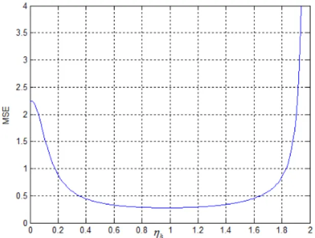
The value of MSE is decreased as ηf increased until ηf

equals 0.9779 (approximately in the mid of stability range). As ηf value increases further, the MSE increases.

This pattern continues till the value of ηf approaches the

stability range limit (ηf≈ 2) the MSE is increased rapidly

and this causes the system to diverge. This result is a perfect match with theoretical stability range of ηf . Fig 8 shows the actual signal and the estimated signal from adaptive RBFNN for ηfequals to 0.9778 (optimal value).

The MSE for this ηf value is minima and equals to 0.276978

Figure 6 Measured current signal (solid) and estimated current signal from Conventional RBFNN (dashed), MSE equals 2.2224

Figure 7MSE for different values of ηf

Secondly, the weight vector of the harmonic component

Wh is only updated, while the weight vector of

fundamental component is remained unchanged (ηf=0),

updating Wh depend on the value ηh. ηh value also is

changed over the whole stability range for η (from 0 to 2), and the mean square error (MSE) is calculated for each value of ηh, as shown in Figure 4.

Figure 8 Measured current signal (solid) and estimated current signal from Adaptive RBFNN (dashed). (ηf=0.9778 and ηh=0)

Figure 9. MSE against h,f equals 0.

Again, the minimum value of MSE is 0.276978 and it is obtained when ηh value is approximately in the middle of

stability range (ηh=0.9779). As ηh value approaches the

stability range limit (ηh ≈ 2) the MSE is increased rapidly and this causes the system to diverge. These are the same results obtained whenηf is only changed. Thirdly, both of

fundamental and harmonic weight vectors are adapted. Fig.10 shows the variation in MSE as ηh is changed for different values of ηf. It can be noticed that the minimum

value of MSE is still the same value that is obtained from changing only ηh or ηf alone (i.e. 0.276978), but this time it occurs with several combinations of ηf and ηh values.

The stability region for changing both ηf and ηh is shown

in Fig.11. The two solid lines represent the range of the stability, which means that any values of ηf and ηh in the

area between the two solid lines maintain the stability of the system, otherwise any combination out of this area will cause system divergence. The equations of the two solid lines are:

ηf + ηh =0 (16) ηf + ηh =2 (17) The combinations of ηf and ηh that give the minimum MSE

are shown also in Fig.6 and they are represented by the dashed line. It is clear that the relation between them is linear and can be given by:

(18) which means that any combination of ηf and ηh satisfies this equation will produce an estimated signal with minimum MSE (MSE= 0.276978), which is the minimum MSE can be achieved of this system.

Figure 10 MSE versus ηhfor different values of ηf

Figure 11The values of ηfand ηh that give the minimum MSE

9778

0

.









Figure 12 The FFT of the measured signal.

Fig. 12 shows the Fast Fourier Transform (FFT) of the measured signal of the fundamental (Fun) and harmonic’s orders components. Fig.13 shows the difference of the FFT component between the measured signal and the estimated signal using the conventional filter (red bar) and the difference between the FFT components of the measured signal and the estimated signal using the adaptive filter (blue bar). This figure prove that adapting technique improves system capability of detecting all the harmonics component, so the improvement of MSE value does not come from improving one harmonic component, but it comes from improvement of all the harmonics components.

Figure 13. The difference between the FFT components between measured signal and conventional filter (red bar) and between measured signal and the adapting filter ( blue bar)

5.2 Effect of the noise

The effect of the noise in the performance of the adaptive RBFNN is investigated in this section. An additive white Gaussian noise is added to the original signal. The

performance of the RBFNN is investigated under three different cases: (i) update only the weight vector of the harmonic component using optimal value for ηh

(ηh=0.9778, ηf=0), (ii) update only the weight vector of

the fundamental component using optimal value for ηf

(ηf=0.9778, ηh=0), and (iii) update both the weight vectors

of the harmonic component and fundamental component using optimal combination for ηh and ηf (ηh+ ηf =0.9778).

The parameter used in this paper to measure the noise level in this paper is Signal to Noise Ratio (SNR), where the SNR in dB is given by:

₍₁₉₎

Where Psignal and Pnoise are the signal and noise power

respectively.

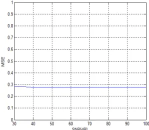
In this paper the SNR level will be changed from 20 db to 100 db. This level is above the common SNR level in electrical power signals that had been adopted in the previous literature, which was above 30 (Đurić & Đurišić, 2010; Liu, Wang, Liu, & Cui, 2016). Figure 14 shows the MSE for several values of signal to noise ratio SNR, the value of h is zero and f is 0.9778 where these values

give a minimum MSE without noise, when the SNR of the measured signal is above 20, the adaptation values still give minimum error, the same curve of Fig.14 is also obtained when the values of are chosen to lie on the line

h +f =0.9778, which shows that the noise with a SNR

greater than or equal to 30dB, didn’t affect the performance of the filter.

Figure 14. MSE against SNR for ηh=0 and ηf =0.9778 In Fig.15 the values of h and f are changed, then the

value of MSE is calculated for a signal has a SNR equals to 30dB, the minimum value of each curve is denoted by ‘*’, if we examine the “*’ points, it is clear that the relation between them is linear since they lie on the same line and

) log( noise signal P p SNR10

the equation of this line is still the same as previous and is given by: h +f =0.9778.

Figure 15MSE against ηhand ηffor SNR=30dB, the ‘*’ represented

the minimum MSE.

5.3 Effect of threshold value

Usually the adapting is required when the error exceeds a certain limit to avoid extra calculations, while in previous sections the threshold value of the error (i.e e(k)=abs(yest(k)-ymeasured(k))) was zero, which means that at each k the value of either h,f or both of

them are modified. In this sectionf are adapted only

when e(k) exceeds a threshold value, the threshold value is changed from 0 to 3, and for each one of them f is

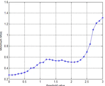
changed, then the MSE is calculated, the results of minimum MSE are shown in Fig. 16 and Fig.17. In Figure 16 x-axis is the threshold value and Y-axis is the minimum MSE value, this value is obtained by changing

f, while Fig.17 shows the value of f that gives the

minimum MSE for each threshold value.

Figure 16 Minimum error for each threshold value

Figure 17 The value of f that gives minimum error for each threshold value

The result in those figures shows that the minimum MSE can be achieved when the threshold value is zero and f

= 0.9778. Even though the MSE is decreased when the threshold value is decreased, but decreasing the threshold value means extra calculations (i.e extra calculation due to adaptation process) as it is shown in Fig. 18, where it shows that the number of calculations is decreased as the threshold value is increased.

Figure 18 Number of calculations for different values of threshold value (constant adaptation coefficient).

6. Conclusions

In this paper, the stability and performance enhancement of adaptive RBFNN is investigated. Adapting the weight vectors of the fundamental and harmonic components based on LMS algorithm improve RBFNN capability to estimate output signal from a power electronic circuit, which is totally different from the signal that the RBFNN is trained for, the stability range of the adapting parameters ηf and ηh are investigated and by

carefully selecting these values, the MSE between the estimated and the measured signal is minimized. The adapting RBFNN shows the capability for disturbance rejection even when the signal has 30 to 100 dB SNR of

Gaussian noise. Further investigating for the adaptive RBFNN is carried out by exploring the effect of the adapting trigger threshold to prevent excessive calculations.

References

Akagi, H. (1996). New trends in active filters for power conditioning.

Industry Applications, IEEE Transactions on, 32(6), 1312–1322. Akagi, H., Watanabe, E. H., & Aredes, M. (2007). The Instantaneous Power Theory. Instantaneous Power Theory and Applications to Power Conditioning. Wiley-IEEE Press.

Almaita, E. (2016). Harmonic Assessment in Jordanian Power Grid Based on Load Type Classification, 11, 58–64.

Almaita, E., & Asumadu, J. A. (2011a). Dynamic harmonic identification in converter waveforms using radial basis function neural networks (RBFNN) and p-q power theory. 2011 IEEE International Conference on Industrial Technology.

Almaita, E., & Asumadu, J. A. (2011b). On-line harmonic estimation in power system based on sequential training radial basis function neural network. 2011 IEEE International Conference on Industrial Technology.

Almaita, E. K. H. (2012). Adaptive Radial Basis Function Neural Networks-Based Real Time Harmonics Estimation and PWM Control for Active Power Filters.

Chang, G. W., Chen, C. I., & Teng, Y. F. (2010). Radial-basis-function-based neural network for harmonic detection. IEEE Transactions on Industrial Electronics, 57(6), 2171–2179. Đurić, M. B., & Đurišić, Ž. R. (2010). Combined Fourier and zero crossing

technique for frequency measurement in power networks in the presence of harmonics.

Haykin, S. S. (1999). Neural networks : a comprehensive foundation. Upper Saddle River, N.J.: Prentice Hall.

Izhar, M., Hadzer, C. M., Masri, S., & Idris, S. (2003). A study of the fundamental principles to power system harmonic. National Power Engineering Conference, PECon 2003 - Proceedings, 225– 232.

Kasabov, N. K. (1996). Foundations of neural networks, fuzzy systems, and knowledge engineering. Cambridge, Mass.: MIT Press. Retrieved from

Liu, Y., Wang, X., Liu, Y., & Cui, S. (2016). Resolution-Enhanced Harmonic and Interharmonic Measurement for Power Quality Analysis in Cyber-Physical Energy System. Sensors, 16(7), 946. Moody, J., & Darken, C. J. (1989). Fast learning in networks of

locally-tuned processing units. Neural Computation, 1(2), 281–294. Rahmani, S., Hamadi, A., & Al-Haddad, K. (2009). A new combination of

shunt hybrid power filter and thyristor controlled reactor for harmonics and reactive power compensation. 2009 IEEE Electrical Power and Energy Conference, EPEC 2009, (1), 1–6. Sumaryadi, Gumilang, H., & Susilo, A. (2009). Effect of power system

harmonic on degradation process of transformer insulation system. Proceedings of the IEEE International Conference on Properties and Applications of Dielectric Materials, 261–264. Wang, Y., Wong, M., & Member, S. (2015). Historical Review of Parallel

Hybrid Active Power Filter for Power Quality Improvement.

Tencon 2015, 5–15.

Yasmeena, & Das, G. T. R. (2016). A review of UPQC topologies for reduced DC link voltage with MATLAB simulation models. 1st International Conference on Emerging Trends in Engineering, Technology and Science, ICETETS 2016 - Proceedings.

Yousef, R., & Hindi, K. (2005). Training radial basis function networks using reduced sets as center points. International Journal of Information Technology, 2(1), 21–35.

Zhang, S. Z. S., Li, D. L. D., & Wang, X. W. X. (2010). Control Techniques for Active Power Filters. Electrical and Control Engineering (ICECE), 2010 International Conference on, 850, 3493–3498. 0 Zouidi, A., Fnaiech, F., AL-Haddad, K., & Rahmani, S. (2008). Adaptive

linear combiners a robust neural network technique for on-line harmonic tracking. Proceedings - 34th Annual Conference of the IEEE Industrial Electronics Society, IECON 2008, (1), 530–534.