Improving a SVM Meta-classifier for Text Documents by using Naive
Bayes
D. Morariu, R. Cre¸tulescu, L. Vin¸tan
Daniel Morariu, Radu Cre¸tulescu, Lucian Vin¸tan "Lucian Blaga" University of Sibiu
Engineering Faculty,Computer Science Department E. Cioran Street, No. 4, 550025 Sibiu, ROMANIA
E-mail: {daniel.morariu,radu.kretzulescu,lucian.vintan}@ulbsibiu.ro
Abstract: Text categorization is the problem of classifying text documents into a set of predefined classes. In this paper, we investigated two approaches: a) to de-velop a classifier for text document based on Naive Bayes Theory and b) to integrate this classifier into a meta-classifier in order to increase the classification accuracy. The basic idea is to learn a meta-classifier to optimally select the best component classifier for each data point. The experimental results show that combining clas-sifiers can significantly improve the classification accuracy and that our improved meta-classification strategy gives better results than each individual classifier. For Reuters2000 text documents we obtained classification accuracies up to 93.87%.
Keywords: Meta-classification, Support Vector Machine, Naive Bayes, Text
docu-ment and Performance Evaluation
1 Introduction
WHILE more and more textual information is available online, effective retrieval is difficult without good indexing and summarization of document content. Document categorization is one solution to this problem. The task of document categorization is to assign a user defined categorical label to a given document. In recent years a growing number of categorization methods and machine learning techniques have been developed and applied in different contexts.
Documents are typically represented as vectors in a features space. Each word in the vocabulary is represented as a separate dimension. The number of occurrences of a word in a document represents the value of the corresponding component in the document’s vector.
In this paper we investigate some strategies for combining classifiers in order to improve the classi-fication accuracy. We used classifiers based on Support Vector Machine (SVM) techniques and based on Naive Bayes Theory, respectively. They are less vulnerable to degrade with an increasing dimensionality of the feature space, and have been shown effective in many classification tasks. The SVM classifiers are actually based on learning with kernels and support vectors.
We combine multiple classifiers hoping that the classification accuracy can be improved without a significant increase in response time. Instead of building only one highly accurate specialized classifier with much time and effort, we build and combine several simpler classifiers.
Several combination schemes have been described in the papers [2] and [6]. A usually approach is to build individual classifiers and later combine their judgments to make the final decision. Another approach, which is not so commonly used because it suffers from the "curse of dimensionality" [5], is to concatenate features from each classifier to make a longer feature vector and use it for the final decision. Anyway, meta-classification is effective only if classifiers’ synergism can be exploited.
In previous studies combination strategies were usually ad hoc and are implementing strategies like majority vote, linear combination, winner-take-all [2], or Bagging and Adaboost [16]. Also, some rather complex strategies have been suggested; for example in [4] a meta-classification strategy using SVM [15] is presented and compared with probability based strategies.
Section 2 and 3 contains prerequisites for the work that we present in this paper. In sections 4 we present the methodology used for our experiments. Section 5 presents the experimental framework and section 6 presents the main results of our experiments. The last section debates and concludes on the most important obtained results and proposes some further work.
2 Support Vector Machine
The Support Vector Machine (SVM) is a classification technique based on statistical learning the-ory [13], [15] that was applied with great success in many challenging non-linear classification problems and on large data sets. The SVM algorithm finds a hyperplane that optimally splits the training set. The optimal hyperplane can be distinguished by the maximum margin of separation between all train-ing points and the hyperplane. Looktrain-ing at a two-dimensional problem we actually want to find a line that "best" separates points in the positive class from points in the negative class. The hyperplane is characterized by a decision function like:
f(x) =sign(hw~,Φ(x)i+b) (1)
wherew~ is the weight vector, orthogonal to the hyperplane, "b" is a scalar that represents the hyper-plane’s margin, "x" is the current sample tested,"Φ(x)"is a function that transforms the input data into a higher dimensional feature space andh·,·irepresents the dot product.Signis the sign function. Ifw~ has unit length, thenhw~,Φ(x)iis the length ofΦ(x)along the direction ofw~. Generallyw~will be scaled by
kw~k. In the training part the algorithm needs to find the normal vector "w~" that leads to the largest "b" of the hyperplane.
3 Naive Bayes
The Bayes classifier uses the Bayes Theorem which basically computes prior probabilities for a given class based on the probability for a given term to belong to the specified class. The classifier computes the probability for a document to be into a given class.
Bayesian theory woks as a framework for making decision under uncertainty - a probabilistic ap-proach to inference [4] and is particularly suited when the dimensionality of the inputs data is high. Bayes theorized that the probability of future events could be calculated by determining their earlier frequency. Bayes theorem states that:
P(Y=yi|X =xk) =
P(Y =yi)P(X =xk|Y =yi)
P(X =xk) (2)
where:
P(Y =yi)- Prior probability of hypothesis Y- Prior
P(X=xk)- Prior probability of training data X-Evidence
P(X=xk|Y =yi)- Probability of X given Y- Likelihood
P(Y =yi|X=xk)- Probability of Y given X- Posterior probability.
The Naive Bayes classifier is based on the simplifying assumption that the attribute values are con-ditionally independent given target value. In other words the assumption is that, given the target value of the instance, the probability of observing the conjunctiony,y...ynis just the product of the probabilities
for the individual attributes:
cmap=argmax<i<mP(X¯ i|Y) =argmax<i<mP(X¯ i) n Y
j= ¯
We used the notation ¯Pfor P because we don’t know exactly the values of the parameters ¯P(Xi)and
¯
P(yj|Xi). These values can be estimated based on the training set.
We can calculate ¯P(Xi) = ||DiD|| , whereDis the set of documents and Di is a subset of D for each
categoryXicontained in the category setX.
For training the classifier we considerV as the words vocabulary from documents contained inD, and for any categoryXi∈X there is a subset of documents contained inDthat belongs toXi category.
Let Yi a vector that contains all words extracted form documents from Di set and ni numbers of all words occurrence fromYi. Thus for each wordyi ∈V we noted with ni j the total number of word
occurrenceyiinYi. We can write:
¯
P(yj|Xi) =
ni j+
ni+|V| (4)
So, basically the Naive Bayes classifier ignores the possible dependencies, correlations, among the inputs and reduces a multivariate problem to a group of simple independent problems. It is noticed that in a Naive Bayes classifier the number of distinctP(y|Xj)terms that must be estimated from the training data is just the number of distinct attribute values multiplied by the number of distinct target values. Therefore it represents a much smaller number than if we would estimate all theP(y,y...yn|Xj)terms
that are needed for Bayesian theory.
For extending the SVM and the Naive Bayes classifiers from two-class classification to multi-class classification, typically one of two methods are used: "One versus the rest", where each topic is separated from the remaining topics, and "One versus the one", where a separate classifier is trained for each class pair as in [17]. We selected the first method for two reasons: first, preliminary experiments shows that the this method gives better performance, which might be explained by the fact that the Reuter’s database contains strongly overlapping classes and assigns almost all samples in more than one class. Second, overall training time is much shorter for the first method.
4 Meta-Classifier Models
In [12] we presented a meta-classifier based on 8 SVM classifiers that was used to improve the accuracy of the classification for text documents. We use the 3 models presented in [11] to test the clas-sification accuracy of the meta-classifier in the case of introducing a new classifier based of naive Bayes theory. The 3 models are: majority vote, the selection based on the Euclidian distance and selection based on the cosine angle.
4.1 Majority Vote (MV)
This first model for meta-classification is a maladjusted model that obtains the same results in time. The idea is to use all selected classifiers to classify the current document. Each classifier proposes a specified class for this document incrementing the corresponding class-counter. The MV meta-classifier will select the class with the greatest count. If two or more classes with identical counts are obtained we classify the current document in all proposed classes.
4.2 Selection based on Euclidean distance (SBED)
This model selects a classifier based on the current input data. It will learn only data that is incorrectly classified by the selected classifier, because we are expecting to have a smaller number of incorrectly classified input data than the number of correctly classified input data. Thus we create for each classifier a queue which contains all incorrectly classified documents.
When we have an input document (current sample) that needs to be classified, first we randomly chose one classifier. After that we compute the Euclidean distances (equation 5) between the current sample and all the samples that are in that self queue of the selected classifier. If we obtain at least one distance smaller than a predefined threshold we will reject this classifier. Instead we will randomly select another classifier, except for the already rejected one. If all component classifiers are rejected, however, we’ll choose the classifier with the greatest Euclidian distance.
Eucl(x,x’) = v u u tXn i= ([x]i− [x0]i) (5)
where[x]i represents the value from entryiof the vectorx, andxandx’represent the input vectors. After selecting the optimal classifier we’ll used it to classify the current sample. If the selected classifier succeeds to correctly classify the current document, nothing is done. Otherwise we’ll put the current document into the corresponding queue. To see if the document is correctly or incorrectly classified we compare our proposed (computed) class with the Reuters proposed class.
The training is as follows: the meta-classifier analyzes the training set and each time when a docu-ment is incorrectly classified, the pattern is added to the selected classifier queue. In the second step, the validation step, we test the classification accuracy using the validation set. In the testing step the char-acteristics of the meta-classifier remains unchanged. Because after each training part the charchar-acteristics of meta-classifier might change, we repeated these two steps many times. After 14 steps we obtain good results and the classification accuracy have not substantially increasing after that.
4.3 Selection based on cosine angle (SBCOS)
The cosine angle is another possibility to compute the document similarity, often used to calculate text similarities. The formula to compute the cosine angleθbetween two input vectorsxandx0is:
cosθ= hx,x0i |x|·|x0| = Pn i=[x]i[x0]i pPn i=[x]i · pPn i=[x0]i (6) where[x]irepresents the value from entryiof a vectorx.
This method is similar with the SBED method with two modifications. Obvious, the first modification is that the similarity between documents is computed using the cosine angle between input vectors. The second modification is that the classifier is not randomly selected. Instead doing this we constantly take into consideration all available classifiers. We compute the cosine between the current sample and all incorrect classified samples that are in the self queues. It is chosen the classifier that obtains the maximum cosine value.
5 Experimental Framework
5.1 The Dataset
Our experiments are performed on the Reuters-2000 collection [14], which has 984Mb of newspapers articles in a compressed format. Collection includes a total of 806,791 documents, with news stories published by Reuters Press covering the period from 20.07.1996 through 19.07.1997. The articles have 9822391 paragraphs and contain 11522874 sentences and 310033 distinct root words. Documents are pre-classified according to 3 categories: by the Region (366 regions) the article refers to, by Industry Codes (870 industry codes) and by Topics proposed by Reuters (126 topics, 23 of them contain no articles). Due to the huge dimensionality of the database we will present here results obtained using a subset of data. From all documents we selected the documents for which the industry code value is
equal to "System software". We obtained 7083 files that are represented using 19038 features and 68 topics. A document is represented as a vector of words, applying a stop-word filter (from a standard set of 510 stop-words) and extracting the word stem [1]. Entire set of 7083 documents is represented as word frequency matrix where each row represents a single document and each column represents a single word [3]. From these 68 topics we have eliminated those topics that are poorly or excessively represented. Thus we eliminated those topics that contain less than 1% documents from all 7083 documents in the entire set. We also eliminated topics that contain more than 99% samples from the entire set, as being excessively represented. After doing so we obtained 24 different topics and 7053 documents, that were split randomly in training set (4702 samples) and testing set (2351 samples). In the feature extraction part we take into consideration both the article and the title of the article.
5.2 Kernel Types for SVM
The idea of the kernel trick is to compute the norm of the difference between two vectors in a higher dimensional feature space without representing those vectors in the new feature space. In practice we observed that by adding a constant bias to the kernel we obtained improved classifying results. For more details please consult [7] and [10].
We used in our selected SVM classifiers two types of kernels each of them with different parame-ters [10]. For the polynomial kernel we varied the degree and for the Gaussian kernel we changed the parameter C according to the following formulas (xandx0being the input vectors):
• Polynomial
k(x,x0) = (·d+hx·x0i)d (7) dbeing the only parameter to be modified and represents the degree of the kernel,
• Gaussian (radial basis function RBF)
k(x,x0) =exp(−kx−x0k
n·C ) (8)
Cbeing the classical parameter andnbeing the new parameter, introduced by us, representing the number of elements from the input vectors that are greater than 0.
For feature selection with Support Vector Machine method we used the polynomial kernel with de-gree 1 [8] and [9].
5.3 Representing the input data
Also in our selected classifier we used different representation of the input data. After extensive experiments [8], [10] we have seen that different types of kernels work better with different types of data representation. We represented the input data in three different formats. In the following formulasn(d,t) is the number of times that termtoccurs in documentd, andn(d,τ)is the maximum frequency occurring in documentd.
• Binary representation- in the input vector we store "0" if the word doesn’t occur in the document and "1" if it occurs without considering the number of occurrences.
• Nominal representation- we compute the value of the weight using the formula: T F(d,t) = n(d,t)
• Cornell SMART representation- we compute the value of the weight using the formula: T F(d,t) ={ i f n(d,t)=
+log(+log(n(d,t)) otherwise (10) These are later called as BIN, NOM or CS.
6 Experimental Results
In [11] it is presented a meta-classifier based on 8 of SVM classifiers that was used to improve the classification accuracy of text documents. The maximum classification accuracy, 87.11%, was obtained by a single SVM type classifier with a second degree for polynomial kernel and Cornell Smart data rep-resentation. In [12] there are presented and tested several types of SVM classifiers based on polynomial kernel and Gaussian kernel, with different forms of representation. From all the tested classifiers eight distinct SVM classifiers were included in the meta-classifier. The eight classifiers were chosen based on the obtained classification accuracy.
We decided to incorporate also a Bayes classifier in the meta-classifier presented above. As a result the new meta-classifier has 9 classifiers. We run again the tests for all the 3 models of the meta-classifier. We also calculated the maximum theoretical limit that could be reached by the new developed meta-classifier. Thus, the introduction of the Bayes classifier in the meta-classifier increases this maximum limit to 98.63% (against 94.21% as it was without Bayes classifier). This fact provides an opportunity to obtain better classification accuracy.
6.1 Selection based on the vote majority
Using this method, the obtained classification accuracy is 86.09%, for the 9 classifiers system. The classification accuracy dropped against the obtained value with 8 classifiers (86.38%), leading to a fall of 0.29%. This may occur because the Bayes classifier obtains - on the entire set of tests - an accuracy of only 81.32%, incorrectly classifying quite a lot of documents (439). Consequently, it seems to "help" the meta-classifier by selecting the 7 cases of wrong categories because Bayes reinforced the wrong vote. The results are shown in Fig. 1.
6.2 Selection based on Euclidian distance (SBED)
We present the results obtained with the new meta-classifier consisting of 9 classifiers in comparison with the meta-classifier presented in [11]. There are presented only the first 14 steps since after this number of steps the classification accuracy is not substantially amended. As in [11] the threshold for the first 7 steps was chosen equal to 2.5 and the threshold for the last 7 steps was chosen equal to 1.5. A step represents a training process followed by a testing process. Fig. 1 shows the results for the meta-classifiers with 8 and 9 classifiers.
For the classifier with 9 classifiers, the results are weaker than those obtained by the meta-classifier with 8 meta-classifiers. This poorer accuracy is due to the poor accuracy of the Bayes meta-classifier (81.32%) compared with the SVM, and due to the fact that the classifiers are randomly selected as we already explained.
Besides, it could be observed that the classification accuracy for the meta-classifier with 9 classifiers has also decreasing trends. This may be due to the fact that a classifier that correctly classifies a document dcould incorrectly classify a documentdthat is quite similar withd. From this reason - when running again the tests set - this classifier has not been selected for the classification ofd(because it gave poor results ford) and then looking for other classifier (which may in turn be classified wrong).
Classification accuracy for Meta-classifier 76 78 80 82 84 86 88 90 92 94 1 2 3 4 5 6 7 8 9 10 11 12 13 14 Steps A c c u ra c y (% )
Majority Vote_8 classifiers Majority Vote_9 classifiers SBED _8 classifiers SBED _9 classifiers
Figure 1: Meta-classifier accuracy for Majority Vote and SBED
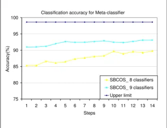
6.3 Selection based on Cosine (SBCOS)
Fig. 2 shows the results, obtained with the new meta-classifier containing 9 classifiers compared with the meta-classifier with 8 classifiers. It presents only the first 14 steps, because after this number of steps, the classification accuracy is not substantially amended. Similar to [11], the threshold for the first 7 steps was chosen equal to 0.8 and the threshold for the last 7 steps was chosen equal to 0.9. In addition, this figure shows the maximum limit that can be achieved by the new meta-classifier (98.63%).
Classification accuracy for Meta-classifier
75 80 85 90 95 100 1 2 3 4 5 6 7 8 9 10 11 12 13 14 Steps A c c u ra c y (% ) SBCOS_ 8 classifiers SBCOS_ 9 classifiers Upper limit
Figure 2: Meta-classifier accuracy for SBCOS and upper limit
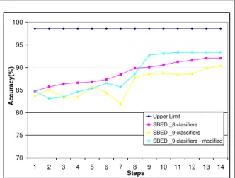
6.4 The modification of the meta-classifier when it fails to select a class
The meta-classifier presented in [11], in the case of a documentdnthat needs to be classified, takes
each classifier and calculates the distance betweendnand each document from the error queue
respec-tively. If the calculated distance is less than the established threshold, the meta-classifier will not use the classifier to classify the documentdn. On the other hand, if all classifiers are rejected by this method,
the meta-classifier will choose the one that has the greatest distance achieved. Thus, the meta-classifier will compute (predict) the class specified by the classifier even if it has a high probability to be wrong. For this reason we modified the meta-classifier in such a way that when all classifiers are rejected, the "forced" selected classifier will not choose the class with the highest value (it will fail anyway because
it is prone to falsely classify that type of documents). Instead, it will choose the class immediately fol-lowing in the list of classes which it predicts. This can be done because the classifier returns different values for each class. In this case, we will not select (predict) the class with the maximum value; instead of doing this, we will select (predict) the class that have the second value in the list, if the difference between the maximum value and the second one is not greater that 0.5. In this case, the classifier would specify another class for the current documentdn. By implementing this change, the results of the
meta-classifier consisting of 9 meta-classifiers have been improved. In the following paragraphs, we will call this meta-classifier: the modified meta-classifier with 9 classifiers.
70 75 80 85 90 95 100 1 2 3 4 5 6 7 8 9 10 11 12 13 14 Steps A c c u ra c y (% ) Upper Limit SBED _8 clasifiers SBED _9 classifiers SBED _9 clasifiers - modified
Figure 3: Classification accuracy for modified meta-classifier- SBED
Fig.3 shows the results obtained with the modified classifier with 9 classifiers vs. the meta-classifier with 8 SVM meta-classifiers and the unmodified meta-meta-classifier with 9 meta-classifiers respectively, all using SBED method. For the selection based on majority voting, learning not being involved, the mod-ifications of the meta-classifier will produce no influence on the final outcome. Besides each figure it is shown the maximum limit that can be obtained by the meta-classifier with 9 classifiers.
The results obtained by the modified meta-classifier with 9 classifiers based on Euclidian distance were improved. Thus, it has been obtained a classification accuracy of 93.32% compared with the un-modified classifier which achieved only 90.38%. Recall that under the same conditions, the meta-classifier with 8 SVM type meta-classifiers [11] obtained a maximum classification accuracy of only 92.04%. In the first 7 steps, the classification accuracy of the modified meta-classifier with 9 classifiers is almost identical to that of the unmodified meta-classifier with 9 classifiers. This happens because during the first steps we can find a classifier that can be selected to classify the current document. After the first 9 steps we put in the queue of each classifier the documents with problems and only after these steps all the basic classifiers could be rejected and the proposed modification to the meta-classifier might be applied. Therefore, during the first steps the results between the two meta-classifiers are slightly different because they always choose a random classifier of the existing 9. With this random selection at different running time we obtain small different results.
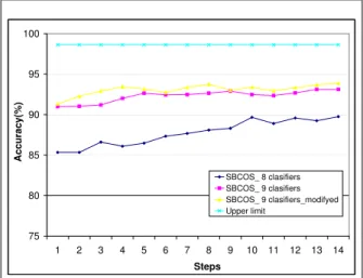
Fig. 4 exposes results obtained by meta-classifier using SBCOS method.
In this case, the classification accuracy for the new meta-classifier has improved from 93.10% to 93.87%. Note that the meta-classifier with 8 SVM classifiers under the same conditions, obtained a classification accuracy of only 89.74%.
75 80 85 90 95 100 1 2 3 4 5 6 7 8 9 10 11 12 13 14 Steps A c c u ra c y (% ) SBCOS_ 8 clasifiers SBCOS_ 9 clasifiers SBCOS_ 9 clasifiers_modifyed Upper limit
Figure 4: Classification accuracy for modified meta-classifier - SBCOS
7 Conclusions and Further Work
Building up on the meta-classifier presented in [11], based on 8 SVM components, we add to these a new Bayes type classifier which leads to a significant improvement of the upper limit that the meta-classifier can reach. Thus, the meta-meta-classifier upper limit has increased from 94.21% when using 8 SVM classifiers [11] to 98.63% when using the 8 SVM classifiers plus the Bayes classifier.
Furthermore, we presented results for all three models of meta-classifiers: majority voting (MV), selection based on Euclidian distance (SBED) and selection based on Cosine (SBCOS). In the case of MV, we obtained a classification accuracy of only 86.09%, which is 0.29% lower than when using only 8 classifiers.
Moreover, in the case of the 9-classifiers SBED meta-classifier we obtained even lower results, on average dropping from 92.04% to 90.38%. In the case of the 9-classifiers SBCOS, the classification accuracy of the meta-classifier has increased from 89.74% to 93.10%.
Finally, we considered that if there is any suspicion that the class to be predicted will not be the correct one, then the classifier should predict a different class. The latest will be the next class in the list of classes only if it is sufficiently close to the first predicted class. These change led to a substantial improvement of the meta-classifier with 9 classifiers. We have performed only experiments with the meta-classifier with 9 classifiers because only in this situation a maximum accuracy of 98.63% could be reached. In the case of the SBED meta-classifier, we obtained an average classification accuracy of 93.32%. This accuracy is with 2.94% greater than the best accuracy obtained without changing the class selection method. In the case of the augmented SBCOS meta-classifier we similarly improved the accuracy from 93.10
In the future, an interesting natural extension of our work may be a more adaptive and intelligent meta-classifier that uses a neural network for choosing the classifier that will be used in classifying the current document. The meta-classifier could learn the incorrect / correct document classified and, without using the error queues, could optimally and faster select the optimal classifier that will be used.
Acknowledgements This work was partially supported by the Romanian National Council of
Bibliography
[1] S. Chakrabarti, Mining the Web- Discovering Knowledge from hypertext data,Morgan Kaufmann Press, 2003.
[2] N. Dimitrova, L. Agnihotri and G. Wei, Video Classification Based on HMM Using Text and Face, Proceedings of the European Conference on Signal Processing,Vol. XVII, pp. 1373-1376, Finland, 2000.
[3] J. Engler, A. Kusiak, Mining Authoritativeness of Collaborative Innovation Partners,International Journal of Computers, Communications and Control, Vol. V, No. 1, pp. 42-51, 2010.
[4] D. Lewis, Naive (Bayes) at Forty: The Independence Assumption in Information Retrieval,ATT Lab Research, NJ, Vol. 1398, pp. 4-15, USA, 1998.
[5] W.H. Lin, A. Houptmann, News Video Classification Using SVM-based Multimodal Classifier and Combination Strategies,Proceedings of the tenth ACM international conference on Multimedia, pp. 323-326, 2002.
[6] W.H. Lin , R. Jin, A. Houptmann, A Meta-classification of Multimedia Classifiers, International Workshop on Knowledge Discovery in Multimedia and Complex Data, Taiwan, 2002.
[7] D. Morariu, L. Vintan, A Better Correlation of the SVM kernel’s Parameters,Proceeding of the 5th RoEduNet International Conference, Sibiu, pp. 244-249, June 2006.
[8] D. Morariu, L. Vintan, V. Tresp, Feature Selection Methods for an Improved SVM Classifier, Pro-ceedings of the 14th International Conference on Computational and Information Science, pp. 83-89, Prague, August 2006.
[9] D. Morariu, L. Vintan, V. Tresp, Evolutionary Feature Selection for Text Documents Using the SVM, Proceeding of the 3rd International Conference on Neural Computing and Patter Recognition, pp. 215-221, Barcelona, October 2006.
[10] D. Morariu, Classification and Clustering using Support Vector Machine, 2nd PhD Report, University "Lucian Blaga" of Sibiu, September, 2005, http://webspace.ulbsibiu.ro/daniel.morariu/html/Docs /Report2.pdf.
[11] D. Morariu, L. Vintan, V. Tresp, Meta-Classification using SVM Classifiers for Text Documents, The 3rd International Conference on Neural Computing and Patter Recognition, pp. 222-227, Barcelona, October 2006.
[12] D. Morariu, Text Mining Methods based on Support Vector Machine,MatrixRom, Bucharest, 2008. [13] C. Nello, J. Swawe-Taylor, An introduction to Support Vector Machines, Cambridge University
Press, 2000.
[14] Reuters Corpus: http://about.reuters.com/researchandstandards/corpus/. Released in November 2000.
[15] B. Schoelkopf, A. Smola, Learning with Kernels. Support Vector Machines,MIT Press, London, 2002.
[16] G. Siyang, L. Quingrui, M. Lin, Meta-classifier in Text Classification, http://www. comp.nus.edu.sg/ zhouyong/papers/cs5228project.pdf.
[17] R. Stoean, C. Stoean, M. Preuss, D. Dumitrescu, Evolutionary Multi-class Support Vector Machine for Classification,International Journal of Computers, Communications and Control, 1(S):423-428, 2006.
Daniel I. MorariuPhD, was born at September 17th 1974 in Sighi¸soara, Romania. He graduates "Lucian Blaga" University of Sibiu, obtaining a M.Sc. in Computer Engineering, and a Ph.D. in Computer Science from the same university. The PhD title is "Contributions to Automatic Knowl-edge Extraction from Unstructured Data", PhD supervisor Professor Lucian N. VINTAN. The PhD program was partially supported from scientific and financial point of view by SIEMENS Corpo-rate Technology from Munich. At present he is a full-time lecture at "Lucian Blaga" University of Sibiu, Engineering Faculty, Computer Science department. He published over 12 scientific papers in international conference from Romania, Czech Republic, and Spain.
R. Cre¸tulescu was born at August 8th 1968 in Sibiu, Romania. He graduates "Babe¸s-Bolyai" University of Cluj-Napoca and obtained a M.Sc. in Computer Engineering, from the "Lucian Blaga" University of Sibiu. At the present time he is a full-time lecture at University of Sibiu, Engineering Faculty, Computer Science department. He published over 6 scientific papers in international conferences from Romania, Finnland and Greece.
Profesor Lucian N. Vin¸tan PhD ("Lucian Blaga" University of Sibiu, RO) is an active researcher in Advanced Computer Architecture, Context Prediction in Ubiquitous Computing Systems, Text Documents Classification, etc. He is a member of Academy of Technical Sciences from Romania, European Commission Expert in Computer Science, and Visiting Researcher Fellow at University of Hertfordshire, UK. Professor Vintan published 8 books and over 100 scientific papers (Romania, USA, Italy, UK, Portugal, Hungary, Austria, Germany, Poland, China etc.). For his merits, Pro-fessor Vintan obtained the "Tudor Tanasescu" Romanian Academy Award. He introduced some well-known original architectural concepts in Computer Architecture domain (Dynamic Neural Branch Prediction, Pre-Computed Branches, Value Prediction focused on CPU’s Context, etc.), recognized, cited and debated through over 80 papers published in many prestigious international conferences and scientific reviews (ACM, IEEE, IEE, etc.)