Kernel Sequential Monte Carlo
Ingmar Schuster?1, Heiko Strathmann?2, Brooks Paige3, and Dino Sejdinovic4 1
FU Berlin,[email protected]
2
Gatsby Unit, University College London,[email protected]
3 Alan Turing Institute and University of Cambridge,
4
University of Oxford and Alan Turing Institute,[email protected]
Abstract. We propose kernel sequential Monte Carlo (KSMC), a frame-work for sampling from static target densities. KSMC is a family of sequential Monte Carlo algorithms that are based on building emulator models of the current particle system in a reproducing kernel Hilbert space. We here focus on modelling nonlinear covariance structure and gradients of the target. The emulator’s geometry is adaptively updated and subsequently used to inform local proposals. Unlike in adaptive Markov chain Monte Carlo, continuous adaptation does not compromise convergence of the sampler. KSMC combines the strengths of sequental Monte Carlo and kernel methods: superior performance for multimodal targets and the ability to estimate model evidence as compared to Markov chain Monte Carlo, and the emulator’s ability to represent targets that exhibit high degrees of nonlinearity. As KSMC does not require access to target gradients, it is particularly applicable on targets whose gradients are unknown or prohibitively expensive. We describe necessary tuning details and demonstrate the benefits of the the proposed methodology on a series of challenging synthetic and real-world examples.
1
Introduction
Monte Carlo methods for estimating integrals have become one of the main inference tools of statistics and machine learning over the last thirty years. They are used to numerically approximate intractable integrals with respect to Bayesian posterior distributions. Importantly, they also provide means to quantify uncertainty in the form of variance estimates, credible intervals and regions of high posterior density. The most widely adopted Monte Carlo method is Markov Chain Monte Carlo (MCMC), which constructs a Markov chain that admits the desired target as its stationary distribution; MCMC generates approximate samples from the target when the chain is run sufficiently long. Poorly tuned MCMC samplers may need to run ‘burn in’ for a very long time before reaching its equilibrium distribution, and successive samples may be highly correlated.
In contrast, sequential Monte Carlo (SMC) methods are based on iterative importance sampling, and have traditionally been applied to inference in filtering
?
Equal contribution
problems with a sequence of time-varying target distributions [9], e.g. in state-space models, where each intermediate distribution is typically defined on a successively larger latent space. In this paper, we focus on static SMC methods, which recently have generated increasing interest as an alternative to MCMC for Bayesian inference on a single target distribution [3, 4, 6, 11]. Static SMC frames inference over a fixed target distribution as a sequential problem by defining an artificial series of incremental targets. This can be done by tempering the target density [6], by including data points sequentially [4], or by targeting the full density at every iteration. The latter is a special case known as population Monte Carlo [PMC, 2].
Kernel methods have recently been employed to construct efficient adaptive MCMC algorithms: via modelling a Markov chain trajectory in a reproducing kernel Hilbert space (RKHS) and using geometry therein, it is possible to sig-nificantly improve mixing on target distributions with nonlinear interactions between components. Covariance in the RKHS can be used to construct an adaptive random walk scheme, kernel adaptive Metropolis Hastings (KAMH), with proposals that are locally aligned with the target density [20]. Gradients of exponential families in the RKHS can be used to construct kernel Hamiltonian Monte Carlo (KHMC), an algorithm that behaves similar to Hamiltonian Monte Carlo (HMC) but without requiring access to gradient information [22]. Both KAMH and KHMC fall back to a random walk in yet unexplored regions, inher-iting convergence properties such as geometric ergodicity on log-concave targets [c.f. Proposition 3 in 22].
In this paper, we develop a framework for kernel sequential Monte Carlo (KSMC) for sampling from static models. Similarly to the previous work in adaptive MCMC [20, 22], KSMC represents the (weighted) particle system of SMC algorithms in a RKHS. The learned geometry of the corresponding ‘emulator’ model is used to construct proposal distributions for both MCMC rejuvenation and importance sampling steps inside SMC.
We apply this framework to two existing SMC algorithms, combining the strengths of SMC with those of kernel adaptive MCMC. Firstly, we introduce kernel adaptive sequential Monte Carlo (KASMC), where the global covariance estimate in the adaptive SMC sampler [ASMC, 11] is replaced by a kernel-informed local covariance [20]. Similar to ASMC, KASMC’s proposals start as a standard random walk and then smoothly transition to taking locally aligned steps. As a result, sampling efficiency can be significantly improved over ASMC. Secondly, we use an infinite dimensional exponential family model [21] to estimate target gradients as in Strathmann et al. [22]. This results inkernel gradient importance sampling (KGRIS), a gradient-free version of gradient importance sampling (GRIS) [19]. KGRIS is a novel adaptation of kernel gradient estimation ideas for constructing Langevin diffusions, and inherits their sampling efficiency compared to random walks. Our contribution includes crucial implementation details, such as Rao-Blackwelisation, stratification, and tuning of the presented algorithms.
Unlike for Langevin diffusions or Hamiltonian dynamics, our framework does not require gradients or higher-order information of the target. Consequently, the
Algorithm 1 Sequential Monte Carlo for Static Models
Input:Sequence of target densitiesπ0, . . . , πT(whereπT=π), size of particle system
N
Output:setsX1, . . . ,XT andW1, . . . ,WT of samples and accompanying weights InitialiseX0toN samples fromπ0, andW0to equal weights 1/N
fort= 1 throught=T do f
Wt={Wt−1i πt(Xt−1i )/πt−1(Xt−1i )}Ni=1
constructXet by re-sampling (Xt−1,Wft), resulting inN copies of samples inXt−1 construct or update proposalqt
if using an MH transition kernelthen
SetXt to
{Xi
t∼MH kernel with proposalqt(·|Xeti)}Ni=1
Wt={1/N}Ni=1
else
SetXt toN samples from
qMixtt (·) = N1 P N i=1qt(·|Xe
i t)
Wt={πt(Xt,i)/qtMixt(Xt,i)}Ni=1
end if end for
returnX1, . . . ,XT andW1, . . . ,WT
KSMC framework is particularly useful in combination with importance sampling frameworks such as SMC2 [5] and IS2 [23] for sampling from doubly intractable targets, where gradient information is unavailable.
We finally argue that (adaptive) SMC is a more natural framework for employing RKHS-based representations. Adaptive MCMC samplers require a vanishing adaptation schedule in order to ensure convergence to the correct target [18], creating a difficult to tune exploration-exploitation trade-off with limited principled guidance on selecting such adaptation schedules. In contrast, SMC proposals can continuously be adapted and the choice of an adaptation schedule is thus entirely circumvented. An easy to use Python package implementing the proposed methods is available under an open source licence.1
2
Background
Sequential Monte Carlo algorithms [6, 8] approximate a target density π by iteratively targeting a sequence of incremental densitiesπ0, . . . , πT, withπT =π. These incremental densities are typically defined such that the initial density
π0 is easy to sample from (e.g. the prior in a Bayesian model). Consecutive distributions πt, πt+1 are ‘close’, in the sense that drawing samples fromπt+1 given samples from πt is easier than drawing samples from πt+1 directly. At each stage t, we approximate the target density πt with a set of N samples
1
Xt={Xti}Ni=1 with associated importance weightsWt={Wti}Ni=1, with ˆ πt(X) = N X i=1 WtiδXi t(X) (1) whereδXi
t is a Dirac point mass onX
i
t. In contrast to SMC as applied to state space models, in a static SMC setting each target density πt is defined on the same space X.
We initialise the algorithm by sampling an initial set ofN samplesX0 from the initial densityq0, with equal importance weights1/N. For each subsequent
t= 1, . . . , T, given a particle set (Xt−1,Wt−1) approximatingπt−1, we construct
a new particle set which approximatesπt. This is a three-step process, summarised in Algorithm 1. First, we re-weight each particle relative to the new target density, setting f Wti=Wti−1 πt(X i t−1) πt−1(Xti−1) .
Weighting the points inXt−1 by{Wfti}Ni=1 yields an approximation toπtin the same manner as in (1) — the new importance weights correct for the change fromπt−1 toπt.
Static SMC then applies re-sampling, constructing an equally-weighted set of particlesXte ={Xeti}Ni=1 by sampling with replacement fromXt−1 with weights proportional toWfti, [7]. Together, these samples form an approximation to πt,
where values from Xt−1 with high weight underπt have been duplicated and those with low weight underπt−1have been discarded. This duplication of values, however, can lead to a sample impoverishment problem: many of the re-sampled valuesXeti may have identical values. This can be avoided by applying a so-called
rejuvenation step after re-sampling [4], constructing an overall approximation (Xt,Wt) toπtwith a diverse set of values ofXti.
The rejuvenation step consists of a proposalqt(Xt|Xt). We here consider twoe
ways of incorporating such a proposal. One traditional option is to use a Markov densityqt as a proposal in a Metropolis-Hastings (MH) kernel which leavesπt invariant: For each Xeti inXt, we propose a new valuee Xti fromqt(Xti|Xeti) and
accept it according to a standard MH acceptance ratio targetingπt. In this case, each importance weight inWtwill be identically1/N.
An alternative is to consider the mixture proposal of all such Markov densities
qtas an importance sampling proposal overπt, a common approach in PMC. We can define qtMixt(Xt) = 1 N N X i=1 qt(Xt|Xeti),
and draw N samples Xt from qMixtt to generate Xt. Now we set importance weights inWtto Wi
2.1 Existing SMC algorithms
In SMC algorithms, we are free in choosing a proposalqt. In contrast to MCMC, it may be directly informed by the previous samples Xt−1 and their weights Wt−1. The following two existing SMC algorithms are examples that we will extend to kernel-based alternatives.
Adaptive SMC The adaptive SMC sampler (ASMC) studied by Fearnhead and Taylor [11] is based on continuously estimating the global covariance Σt of
πt, and updating a scaling parameter ν2. This is done from the re-weighted particle system, which is subsequently moved through a Markov kernel. The proposal distribution used within the MH kernel at pointX in Algorithm 1 is
qt(·|X) =N(·|X, ν2Σ
t+γ2I).
Gradient importance sampling In addition to using the estimated covariance
Σt of π as in ASMC, gradient importance sampling [GRIS, 19] incorporates a drift term based on the log target gradient. For target gradient∇logπand previous sampleX, the proposal distribution in Algorithm 1 isqt(·) =N(·|X+
D(∇logπ(X)), ν2Σt), for each individual particleX in the current (unweighted) particle set. A typical choice for the drift function isD(y) =δywith 0< δ <1. Rather than incorporating a MH step, the updated values are importance weighted — GRIS is a population Monte Carlo (PMC) algorithm. In numerical experiments, GRIS compares favourably to its closest MCMC relatives like the adaptive MALTA algorithm and adaptive Metropolis [19].
2.2 Kernel adaptive MCMC proposals
The previously described SMC algorithms are based on target covariance and gradients. We now review how these quantities were previously modelled using kernel methods in the context of MCMC. Note that any form of adaptation in MCMC requires care in order to preserve ergodicity of the resulting Markov chain, and some form of vanishing adaptation is needed [1, 18]. This can be achieved e.g. by updating the proposal family with vanishing probability [20, 22]. Covariance emulator Sejdinovic et al. [20] introduced a kernel covariance emulator as a method for adapting the proposal distribution in a Metropolis-Hastings MCMC algorithm, based on the history of the Markov chain X={X1, X2, . . .}. The idea is to represent covariance of the target as an empirical Gaussian measure with meanµX:= |X1|PX∈Xk(X,·) and covariance
1
|X|
P
X∈Xk(X,·)⊗k(X,·)−
µX⊗µX in a RKHS with kernelk. This measure can be sampled from exactly,
and it is possible to (approximately) map samples back to the original space. Sejdinovic et al. [20] showed that it is possible to integrate out the RKHS proposal analytically, which elegantly results in aclosed form Gaussian proposal density in the input space. For a Gaussian kernel, the proposal at particleXj locally aligns to the structure of the posterior atXj, and is given by
qKAMH(·|Xj) =N(·|Xj, γ2I+ν2MX,XjCM
>
whereC=I−1 n11
> is a centering matrix andM
X,Xj collects kernel gradients
with respect to all particles,
MX,Xj = 2[∇xk(x, X1)|x=Xj, ...,∇xk(x, XN)|x=Xj].
Additional exploration noise with varianceγ2 avoids that the proposal col-lapses in unexplored regions of the input space.
Gradient emulator To overcome random walk behaviour of KAMH, Strathmann et al. [22] constructed an algorithm that adaptively learns the gradient struc-ture of the Markov chain history, and mimics Hamiltonian dynamics using the learned gradients. This is done by fitting an un-normalised infinite dimensional exponential family model with density function exp(hf, k(x,·)iH−A(f)). Here,
hf, k(x,·)iH=f(x) is the inner product between natural parameters f and
suffi-cient statisticsk(x,·) in a RKHSH, andA(f) is the (intractable) log-partition function. Remarkably, it is possible to efficiently estimatef via minimising the expectedL2error of∇
xf(x) without dealing withA(f). Combining this model with a further approximation, based on random basis functions [KMC finite; 22], allows for efficient on-line updates of the emulator. Similar to Hamiltonian Monte Carlo, the resulting KHMC algorithm offers substantial improvements over random walks. Tt does so, however,without requiring gradient information of the target. This allows application to intractable likelihood models, where we cannot evaluate the target densitiesπt even up to a normalizing constant, and gradients are similarly unavailable.
3
Kernel sequential Monte Carlo
We now develop a kernel sequential Monte Carlo framework. KSMC is based on combining classical adaptive SMC with the emulator based proposals of kernel adaptive MCMC. In general, once a kernel emulator is fitted to past particle systems, we can use it in either of two ways: as proposals for MH rejuvenation steps inside SMC or as importance densities in PMC.
Key contributions. Our main contribution is to combine several yet unconnected pieces of literature into a novel framework that performs favourably compared to its individual parts: adaptive SMC proposals, SMC for intractable likelihoods, and kernel emulators for efficient proposals. This combination is simple yet very natural: As compared to (kernel) adaptive MCMC, the KSMC framework (i) circumvents the need for vanishing adaptation, (ii) can represent multimodality, (iii) allows to estimate model evidence in a straight-forward manner. On the
other hand, as compared to plain adaptive SMC and PMC, the use of kernel emulators (iv) leads to faster convergence for nonlinear targets.
We present two novel algorithms, KASMC and KGRIS, both of which are weighted and kernelised generalisations of existing kernel MCMC and SMC respectively. These modifications can lead to significant mixing improvements in practice. Our contribution furthermore includes variance reduction techniques
that are critical in practice. In particular, naïve implementations can suffer from high variance induced by simplifications. As this results in lower quality emulators, too high variance would be self-reinforcing and is to be strictly avoided.
3.1 Kernel adaptive rejuvenation: KASMC
We can use both kernel emulators for the rejuvenation step of SMC. More specif-ically, at time-stept+ 1, we target distributionπt+1, based on a particle system approximatingπt. After re-weighting, the new system {(Wt+1,i, Xt+1,i)}Ni=1 is a weighted approximation to πt+1. We here focus on the nonlinear covariance emulator which can be either fitted using the equally-weighted re-sampled values
e
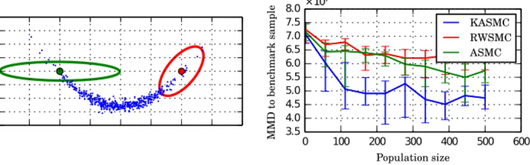
Xt, or the original particle set with weights Wft. The proposal distribution for Algorithm 1 atX then is exactlyqKAMH. As in KAMH, this results in covariance matrices for Gaussian proposals which locally align with the target [20], now taking the SMC particle weights into account. The resulting kernel adaptive SMC sampler (KASMC) inherits KAMH’s ability to explore non-linear targets more efficiently than proposals based on estimating global covariance structure such as in Fearnhead and Taylor [11] and Haario et al. [13]. Figure 1 (left) shows a simple illustration of a global (ASMC) and local proposal distribution (KASMC). Compared to previous work on kernel induced local covariance matrices for MCMC [20], we implement a random features approximation in order to enable computationally efficient updates with information gained from new samples [17].
3.2 Kernel induced importance densities: KGRIS
Another way to use kernel-based emulators is for generating proposals which are corrected by importance sampling, i.e. in PMC. In our second approach, a kernel emulator is fitted to weighted particles, which were previously corrected via importance weights. As an example, we here use the kernel gradient emulator by Strathmann et al. [22], in its finite dimensional approximation (KMC finite), c.f. [22, Proposition 2].
The log density of the approximate estimator takes the simple formf(x) =
θ>φ
x, whereφx∈Rmis an embedding ofxinto anm-dimensional feature space,
andθ∈Rmis estimated by ˆθ=C−1bfrom samplesx. Given a weighted particle system{(Wt,i, Xt,i)}Ni=1, thenb, C are weighted averages of the form
b:=− 1 PN i=1Wt,i N X i=1 Wt,i d X `=1 ¨ φ`x, C:= 1 PN i=1Wt,i N X i=1 Wt,i d X `=1 ˙ φ`x φ˙`x> ,
with element-wise derivatives ˙φ` x := ∂ ∂x`φx and ¨φ ` x := ∂2 ∂x2 `
φx. Note that the estimator can be updated in an online fashion once the particle system changes. Rather than simulating Hamiltonian dynamics to generate a proposal, we here
take single gradient steps, i.e. the Markov density at in Algorithm 1 at X is
qt(·|X) =N(·|X+δ∇f(X), ν2Σt) for some parametersδ >0, ν2>0. This keeps the risk of divergence due to wrongly estimated gradients low. We arrive at kernel GRIS, a gradient-free variant of GRIS [19].
3.3 Controlling emulator variance in PMC
PMC is somewhat sensitive to badly scaled proposals, as these are not rejected as in a Metropolis-Hastings step. In particular for gradient emulators used within PMC, variance reduction is important to avoid numerical divergence. The original PMC paper introduces re-sampling in order to deal with un-weighted instead of weighted samples [2], though at the cost of an increased variance. While some approaches avoid re-sampling altogether [3], we consider re-sampling here as a way to obtain a set of locations{Xeti}Ni=1 for our Markov proposal components of
the mixtureqMixt t (·) = N1
PN
i=1qt(·|Xeti), due to better behaving variance in high
dimension. With re-sampling, Monte Carlo variance only grows asO(D) rather thanO(exp(D)) without re-sampling, whereD is the dimensionality [8].
Given a re-sampled number ofN particles and the updated emulator qt, we simulate from the mixture distribution qMixt
t with stratification, i.e. we draw exactly one sample from each of the equally weighted mixture components. Another view of this scheme is to draw a single realisation from qt(·|Xeti) for
all i= 1, . . . , N and Rao-Blackwellise. Finally, we can view the scheme as an
instance of the deterministic mixture idea [10]. Without this technique, i.e. using weights π(·)/qt(·|Xeti), variance might grow catastrophically large, as too high variance can be self-reinforcing by resulting in emulators of low quality.
4
Evaluation
We empirically evaluate performance of KASMC on a simple non-linear target, on a multi-modal sensor network localisation problem, and in estimating Bayesian model evidence in a model with an intractable likelihood on a real-world dataset. The final experiment uses a challenging stochastic volatility model with S&P 500 data from Chopin et al. [5] to evaluate KGRIS.
For the KASMC experiments on static target distributions, a sequence of incremental target densities can be defined using a geometric bridge withπt∝
π1−ρt
0 π
ρt for some initial distributionπ
0, where (ρt)Tt=1 is an increasing sequence satisfyingρT = 1. The bandwidth parameter of the kernel emulator models is set to the median distance between particles [12].
We also note these algorithms have a free scaling parameter ν2, which we would like to adapt online. To accomplish parameter tuning, we use the standard framework of stochastic approximation for tuning MCMC kernels [1], i.e. tuning acceptance rateαt towards an asymptotically optimal acceptance rateαopt = 0.234 for random walk proposals [18]. After the MCMC rejuvenation step, a Rao-Blackwellised estimate ˆαt of expected acceptance probability is available by simply averaging the acceptance probabilities for all MH proposals. Then,
Fig. 1: Left: Proposal distributions around one of many particles (blue) for each KASMC (red) and ASMC (green). KASMC proposals locally align to the target density while ASMC’s global covariance estimate might result in poor MH rejuvenation moves. Right:Improved convergence of all mixed moments up to order 3 of KASMC compared to using SMC with static or adaptive Metropolis-Hastings steps.
setνt2+1=νt2+λt( ˆαt−αopt) for some non-increasing sequenceλ1, . . . , λT. This strategy of approximating optimal scaling assumes that consecutive targets are close enough so that the acceptance rate when usingν2
t to targetπt provides information about the expected acceptance rate when using ν2
t with targetπt+1. This is discussed further in the supplemental material.
4.1 KASMC: Improved convergence on synthetic nonlinear target We begin by studying convergence of KASMC compared to existing algorithms on a simple benchmark example: the strongly twisted banana-shaped distribution in
D= 8 dimensions used in Sejdinovic et al. [20]. This distribution is a multivariate Gaussian with a non-linearly transformed second component, defined as
B(y;b, v) =N(y1; 0, v)N(y2;b(y12−v),1) D
Y
j=3
N(yj; 0,1).
We compare SMC algorithms using different rejuvenation MH steps: a static random walk Metropolis move (RWSMC) with fixed scaling ν = 2.38/√D, ASMC, and KASMC using a Gaussian RBF kernel. For the latter two algorithms, all particles are used to compute the proposal, and a fixed learning rate of
λ = 0.1 is chosen to adapt scale parameters. Starting with particles from a multivariate Gaussian N(0,502), we use a geometric bridge that reaches the targetB(y;b= 0.1, v= 100) in 20 steps. We repeat the experiment over 30 runs. Figure 1 (right) shows that KASMC achieves faster convergence of the first 3 moments, i.e. in MMD2 distance to a large benchmark sample.
2
The maximum mean discrepancy, here using a polynomial kernel of order 3, quantifies differences of all mixed moments up to order 3 of two independent sets of samples.
4.2 A multi-modal application: sensor network localisation
We next study performance of KASMC on a multi-modal target arising in a real-world application: inferring the locations of S sensors within a network, as discussed in [14, 15]. We here focus on the static case: assume a number of stationary sensors that measure distance to each other in a 2-dimensional space; a distance measurement is successful with a probability that decays exponentially in the squared distance, and the observation is missing otherwise. If distance is measured, it is corrupted by Gaussian noise. The posterior over the unknown sensor locations forms an extremely constrained non-linear and multi-modal distribution induced by the spatial set-up.
AssumeS sensors with unknown locations{xi}Si=1⊆R
2. Define an indicator variableZi,j∈ {0,1} for the distanceYij ∈R+between a pair of sensors (xi, xj) being either observed (Zi,j = 1) or not (Zi,j= 0), according to
Zi,j∼Binom 1,exp −kxi−xjk 2 2 2R2 .
If the distance is observed, thenYij is corrupted by Gaussian noise, i.e.
Yi,j|Zi,j= 1∼ N kxi−xjk, σ2
,
andYi,j= 0 otherwise.
Previously, [14] focussed on MAP estimation of the sensor locations, and [15] focussed on a well-conditioned case (S= 8 sensors andB= 3 base sensors with known locations) that results in almost no ambiguity in the posterior. We argue that Bayesian quantification of uncertainty is more important for cases where noise and missing measurementsdoes notallow to reconstruct the sensor locations exactly. We therefore reuse the dataset from [15] (R= 0.3,σ2= 0.02)3, but only use the first S = 3 locations/observations. In order to encourage ambiguities in the localisation task, we only use the first 2 base sensors of [15] with known locations that each do observe distances to the S unknown sensors but not of each other. Unlike [15], we use a Gaussian priorN(0.5, I) to avoid the posterior being situated in a bounded domain.
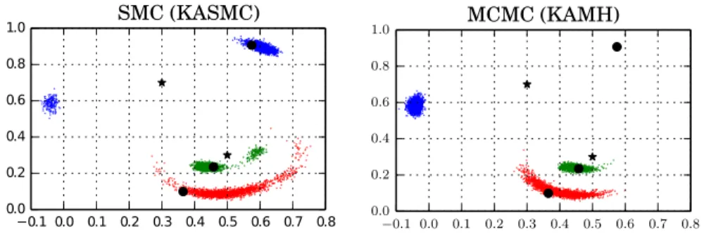
Figure 2 shows the marginalised posterior for one run each of KASMC (SMC) and KAMH (MCMC), where we matched the number of likelihood evaluations (500,000). We run KASMC using 10,000 particles and a bridge length of 50, and MCMC-KAMH for 50×10,000 iterations of which we discard half as burn-in; both were initialized with samples from the prior. Tuning parameters ν2 are set using a diminishing adaptation scheduleλt= 1/
√
tfor KAMH and a fixed learning rate λt= 1 for KASMC. MCMC is not able to traverse between the multiple modes and interpretations of the data, in contrast to SMC.
In order to compare ASMC to KASMC, we created a benchmark sample via running 100 standard MCMC chains (randomly initialised to cover all modes)
3
Downloaded from http://www.ics.uci.edu/~slan/lanzi/CODES_files/ WHMC-code.zipon 8/Oct/2015.
−0.1 0.0 0.1 0.2 0.3 0.4 0.5 0.6 0.7 0.8 0.0 0.2 0.4 0.6 0.8 1.0 MCMC (KAMH)
Fig. 2: Posterior samples of unknown sensor locations (in color) by kernel-based SMC and MCMC on the sensors dataset. The set-up of the true sensor locations (black dots) and base sensors (black stars) causes uncertainty in the posterior. SMC recovers all modes while MCMC does not. The posterior has a clear non-linear structure.
each for 50000 iterations, discarding half the samples as burn-in, and randomly down-sampling to a size of 100. We then compute the empirical MMD distance to the output of the individual algorithms, averaged over 10 runs. For the chosen number of sensors, ASMC and KASMC perform similarly. With less sensors, i.e. more ambiguity, KASMC produces samples with both less MMD distance from a benchmark sample and less variance. For example, for a set-up withS= 2 and 1000 particles, we get a MMD distance to a benchmark sample of 0.76±0.4 for KASMC and 0.94±0.7 for ASMC.
4.3 KASMC: evidence estimation in Gaussian process classification Following Sejdinovic et al. [20], we consider Bayesian classification on the UCI Glass dataset, discriminating window glass from non-window glass, using a Gaussian process (GP). It was found that the induced posterior is indeed non-linear [22, 20]. In Sejdinovic et al. [20], samples from the marginal posterior over GP hyper-parameters were simulated (the GP latent variables integrated out). We emphasise a different point here: KSMC’s ability to estimate the model evidence as compared to KAMH, and its faster convergence compared to ASMC.
Consider the joint distribution of latent variablesf, labelsy(with covariate matrixX), and hyper-parametersθ, given by
p(f,y, θ) =p(θ)p(f|θ)p(y|f),
wheref|θ∼ N(0,Kθ), withKθ modelling the covariance between latent variables evaluated at the input covariates. Consider the binary logistic classifier, i.e.
p(yi|fi) = 1−exp(1−y
ifi) whereyi∈ {−1,1}. In order to perform Bayesian model
selection (i.e. comparing different covariance functions), we need to estimate the model evidence of the marginal posterior given the hyper-parameters. Here, the marginal likelihoodp(y|θ) is intractable for non-Gaussian likelihoodsp(y|f).
Fig. 3: Estimating model evidence of a GP using the IS2 framework. The plot shows the MC variance over 50 runs as a function of the size of the particle system.
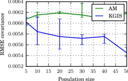
5 10 15 20 25 30 35 40 45 50 Population size 0.0052 0 .0054 0 .0056 0 .0058 0 .0060 0 .0062 0 .0064 R M S E co v a ri a n ce AM KGIS
Fig. 4: Convergence of RMSE for estimat-ing all elements of the posterior covari-ance matrix of the stochastic volatility model.
We estimate model evidence for the GP classifier equipped with a standard Gaussian Automatic Relevance Determination (ARD) covariance kernel; an unbiased estimate can be obtained using importance sampling
ˆ p(y|θ) := 1 nimp nimp X i=1 p(y|f(i))p(f (i)|θ) q(f(i)|θ), (2)
where f(i) in=1imp ∼ q(f|θ) are nimp importance samples, e.g. from a Laplace approximation ofp(f|y, θ). We here do not tune the number of ’inner’ importance samples, but follow [20] and usenimp= 100.
Figure 3 shows that evidence estimates of KASMC exhibit less variance than those of ASMC. The ground truth model evidence was established via running 20 SMC instances using N = 1000 particles and a bridge length of 30, and averaging their evidence estimates. The experiment is performed 50 times, using
N = 100 particles and a bridge length of 20, starting from he prior on the log hyper-parametersπ0 =p(θd)≡ N(0,52). The learning rate is constantλt= 1, and adaptation is towards an acceptance rate of 0.23.
4.4 KGRIS: stochasitic volatility model with intractable likelihood A particularly challenging class of Bayesian inverse problems are stochastic volatil-ity models. As time series models, they often involve high-dimensional nuisance variables, which usually cannot be integrated out analytically. Furthermore, risk management necessitates to account for parameter and model uncertainty, and models have to capture the non-linearities in the data [5]. We here concentrate on the prediction of daily volatility of asset prices, reusing the model and dataset studied by Chopin et al. [5] to evaluate KGRIS. Due to the lack of analytically available gradients for this model, we compare two gradient free PMC versions:
KGRIS and a random walk PMC with global covariance adaptation in the style of Haario et al. [13].
Letstbe the value of some financial asset on dayt, thenyt= 10(5/2)log(st/st−1) is called the log-returns (upscaling for numerical reasons). We model the observed log-returnyt as dependent on a latentvt by the observation equation
yt=µ+βvt+
√
vtt
fort≤1. Heretis a sequence of i.i.d. standard Gaussian errors andvtis assumed to be a stationary stochastic process known as theactual volatility. Chopin et al. [5] develop a hierarchical model forvtbased on the idea of analytically integrating a continuous time volatility model over daily intervals [for details see 5]. Using this construction, the (discrete time)vt is parameterised by stationary meanξ and varianceω2of the so calledspot volatility and the exponential decayλof its auto-correlation. This results in the following model for the actual volatilityvt:
k∼Pois(λξ2/ω2), c1:k ∼U(t, t+ 1), e1:k ∼Exp(ξ/ω2) zt+1=ztexp(−λ) + k X j=1 ejexp(−λ(t+ 1−cj)) vt+1=λ−1 zt−zt+1+ k X j=1 ej , xt+1= (vt+1, zt+1)>
whereztis the discretely sampled spot volatility process and (vt+1, zt+1)> is the Markovian representation of the state process. The variablesk, c1:k ande1:k are generated independently for each time period. Fork= 0, the set 1 :kis defined to be empty. The dynamics implyΓ(ξ2/ω2, ξ2/ω2) to be the stationary distribution forzt, which is also used as the initial distribution onz0. The parameters of the model areθ= (µ, β, ξ, ω2, λ) and the likelihood is intractable. Chopin et al. [5] developed a sampler forθ based on iterated batch importance sampling using nested SMC with pseudo-marginal MCMC moves for integrating out thextand dubbed their approach SMC2.
In our experiment, we use KGRIS proposals in a population Monte Carlo setting, i.e. without resorting to MCMC moves at all. We re-use the code developed for the original SMC2paper in order to integrate out thex
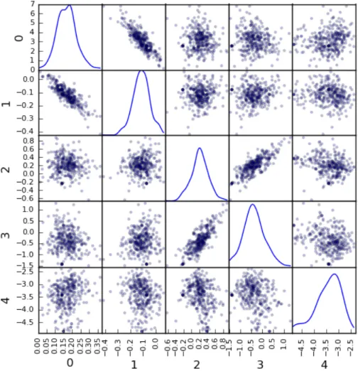
tand thus get likelihood estimates, with the same settings for algorithm parameters. The observedstare the 753 observations from consecutive days of the S&P 500 index also used by Chopin et al. [5]. KGRIS uses a particle system of increasing sizes with each particle going through 100 iterations. See Figure 5 in the Appendix for a plot of the pair-wise marginals of this posterior.
We use the same vague priors as Chopin et al. [5],
µ∼ N(0, σ2= 2), β∼ N(0, σ2= 2), ξ∼Exp(0.2)
Figure 4 shows that the incorporated gradients lead to better performance of KGRIS in estimating the target covariance matrix. This is in-line with the finding that GRIS improves over pure random walk methods [19].
5
Discussion
In this paper, we developed a framework for kernel sequential Monte Carlo. KSMC adaptively learns the target geometry via kernel emulators and subse-quently uses this information for local proposals. KSMC is especially attractive in the case where likelihoods and gradients are intractable. We instantiated two algorithms within KSMC: estimating nonlinear covariance in combination with MCMC rejuvenation and estimating gradients in combination with importance sampling proposals. Both significantly outperform state-of-the-art gradient-free SMC algorithms in practice. We conclude with some discussion on computational complexity, more general usage of the learned emulators, and on the relative benefits of PMC in the kernel setting.
Computational costs & increasing dimensions. While adaptive schemes for SMC (and MCMC) can increase statistical efficiency of the sampling scheme, they impose additional computational costs. Somewhat surprisingly, however, these relatively large costs do not severely impact the efficiency per runtime ratio in practice. The reason is that in the context of intractable likelihoods, the computational cost of fitting a kernel emulator is typically dominated by the larger cost of evaluating model likelihood. In our real-world experiments on GP classification and a stochastic volatility model in Sections 4.3 and 4.4, a profiler reveals that less than 5% of the overall wall-clock time is spent in computing kernel informed proposals. This effect increases with dataset size and model complexity, as evaluating likelihood gets more costly. Clearly however, in the case where we need not resort to pseudo-marginal or SMC2 type samplers, the application of kernel based estimators might result in slower sampling without much gain in Monte Carlo error.
In growing dimensions, the number of data required to sufficiently estimate nonlinear covariance and gradients quickly becomes infeasible. High dimensional sampling problems typically arise in non-parametric models, e.g. Gaussian pro-cesses, where each data point comes with additional parameters. In the intractable likelihood framework that we consider here, however, the marginal posterior over hyper-parameters typically is independent of such latent variables — and there-fore usually of moderate dimension. Random walk methods, which are the default choice for intractable likelihoods, scale badly in high dimensions themselves [16]. Our method is an improvement in the intermediate case: closed form gradients are not available, but the dimensionality of the problem allows to estimate the target geometry just accurately enough to improve mixing. Strathmann et al. [22] reported their gradient estimator to scale up from dozens to a hundred dimensions on laptop computers, depending on smoothness properties of the target. It is an active area of research to further scale up these techniques by exploiting structure in the target density.
Emulators as a posterior approximation. The kernel approximation of the target density could be considered itself as an output of our algorithms, representing the posterior directly instead of using the kernel approximation within a sampler. There are a number of problems with this approach though: firstly, we note that our emulator models do not need to be perfect to generate useful proposals, therefore allowing us to exploit posterior structure much earlier (even with non-perfect model fit) during sampling, still resulting in a correct SMC sampler. Also, approximating integrals of test functions with respect to the posterior using the kernel approximation is not possible in closed form, while it is straight forward using a Monte Carlo sum. For example, assume a log density model f(x) =
P
iαik(xi, x). For the Gaussian kernel k(x, y) = exp(−||x−y||2), the density is the exponential of a sum of Gaussian centred at the points xi. Computing an integral as simple as the posterior mean,µ=Z−1R xexp(P
iαiexp(−||xi−
x||2))dx, already is intractable, even if the evidenceZ were known. Thirdly, it is not possible to sample from the kernel emulator directly using ordinary Monte Carlo. One could imagine running a second MCMC/SMC targeting the emulator model. Not only would this defeat the purpose of the algorithm (this is the problem we are trying to solve in the first place), it also leads to samples that are not guaranteed to consistently estimate posterior expectations unlike kernel SMC or kernel MCMC.
SMC versus PMC for kernel based proposals. The consensus in the wider SMC community is that using an artificial sequence of proposal distributions for sampling from a static target is preferable to the PMC approach. This is based on the fact that the coverage of the final target is better in these tempering-style algorithms. It however results in a considerable computational investment for those iterations where an intermediate target is considered.
We also note that on-line updates of the kernel emulator are not possible: the target changes in every iteration. The contrary is true in PMC, where the the actual distribution of interest is targeted in every iteration. Here, a popular approximation technique of kernels is a good fit: By expressing the emulator model in terms of finite dimensional random Fourier features, we can perform cheap on-line updates [22]. The emulator therefore can accumulate information from all PMC iterations without the computational efforts of re-computing its solution, providing a relative advantage to SMC in this context.
Acknowledgments. I.S. was supported by a PSL postdoc grant and DFG through grant CRC 1114 "Scaling Cascades in Complex Systems", Project B03 "Multilevel coarse graining of multiscale problems". H.S. was supported by the Gatsby Chaitable foundation. B.P. was supported by The Alan Turing Institute under the EPSRC grant EP/N510129/1.
References
1. C. Andrieu and J. Thoms. A tutorial on adaptive MCMC.Statistics and Computing, 18(November):343–373, 2008. ISSN 09603174.
2. O. Cappé, a. Guillin, J. M. Marin, and C. P. Robert. Population Monte Carlo.
Journal of Computational and Graphical Statistics, 13(4):907–929, Dec. 2004. ISSN 1061-8600.
3. O. Cappé, R. Douc, A. Guillin, J.-M. Marin, and C. P. Robert. Adaptive importance sampling in general mixture classes. Statistics and Computing, 18(4):447–459, Apr. 2008. ISSN 0960-3174.
4. N. Chopin. A sequential particle filter method for static models. Biometrika, 89(3): 539–552, 2002. ISSN 0006-3444.
5. N. Chopin, P. E. Jacob, and O. Papaspiliopoulos. SMC2: an efficient algorithm for sequential analysis of state space models. Journal of the Royal Statistical Society: Series B (Statistical Methodology), 75(3):397–426, 2013.
6. P. Del Moral, A. Doucet, and A. Jasra. Sequential Monte Carlo samplers. Journal of the Royal Statistical Society: Series B (Statistical Methodology), 68(3):411–436, June 2006. ISSN 1369-7412.
7. R. Douc and O. Cappé. Comparison of resampling schemes for particle filtering. In
Proceedings of the 4th International Symposium on Image and Signal Processing and Analysis, pages 64–69, 2005. ISBN 953-184-089-X.
8. A. Doucet and A. Johansen. A tutorial on particle filtering and smoothing: Fifteen years later. Handbook of Nonlinear Filtering, (December 2008):4–6, 2009. 9. A. Doucet, N. D. Freitas, and N. Gordon. An Introduction to Sequential Monte
Carlo Methods. 2001.
10. V. Elvira, L. Martino, D. Luengo, and M. F. Bugallo. Generalized Multiple Importance Sampling. Technical report, 2015.
11. P. Fearnhead and B. M. Taylor. An Adaptive Sequential Monte Carlo Sampler.
Bayesian Analysis, (2):411–438, 2013.
12. A. Gretton, K. M. Borgwardt, M. J. Rasch, B. Schölkopf, and A. Smola. A kernel two-sample test. The Journal of Machine Learning Research, 13(1):723–773, 2012. 13. H. Haario, E. Saksman, and J. Tamminen. An Adaptive Metropolis Algorithm.
Bernoulli, 7(2):223–242, 2001. ISSN 13507265.
14. A. T. Ihler, J. W. Fisher, R. L. Moses, and A. S. Willsky. Nonparametric belief prop-agation for self-localization of sensor networks. Selected Areas in Communications, IEEE Journal on, 23(4):809–819, 2005.
15. S. Lan, J. Streets, and B. Shahbaba. Wormhole hamiltonian monte carlo. In
Twenty-Eighth AAAI Conference on Artificial Intelligence, 2014.
16. R. M. Neal. MCMC using Hamiltonian dynamics. InHandbook of Markov Chain Monte Carlo. Chapman & Hall/CRC, 2011.
17. A. Rahimi and B. Recht. Random features for large-scale kernel machines. In
Advances in Neural Information Processing Systems, pages 1177–1184, 2007. 18. J. S. Rosenthal. Optimal Proposal Distributions and Adaptive MCMC. InHandbook
of Markov Chain Monte Carlo, chapter 4, pages 93–112. Chapman & Hall, 2011. 19. I. Schuster. Gradient Importance Sampling. arXiv preprint arXiv:1507.05781, 2015. 20. D. Sejdinovic, H. Strathmann, M. G. Lomeli, C. Andrieu, and A. Gretton. Kernel
Adaptive Metropolis-Hastings. InInternational Conference on Machine Learning (ICML), pages 1665–1673, 2014.
21. B. Sriperumbudur, K. Fukumizu, R. Kumar, A. Gretton, and A. Hyvärinen. Den-sity Estimation in Infinite Dimensional Exponential Families. arXiv preprint arXiv:1312.3516, 2014.
22. H. Strathmann, D. Sejdinovic, S. Livingstone, Z. Szabo, and A. Gretton. Gradient-free hamiltonian monte carlo with efficient kernel exponential families. InNIPS, 2015.
23. M.-N. Tran, M. Scharth, M. K. Pitt, and R. Kohn. Importance sampling squared for Bayesian inference in latent variable models. arXiv preprint arXiv:1309.3339, 2013.
A
Implementation details
In this section, we cover a number of implementation details for using KASMC in practice, such as optimal scaling, adaptive re-sampling and re-weighting between iterations.
A.1 Scaling parameters
Similar to other MH proposals, KAMH has a free scaling parameter denotedν2 which we would like to adapt after one SMC iteration. To accomplish parameter tuning, we use the standard framework of stochastic approximation for tuning MCMC kernels [1], i.e. tuning acceptance rate αt towards an asymptotically optimal acceptance rate αopt = 0.234 for random walk proposals [18]. More precisely, after the MCMC rejuvenation step, a Rao-Blackwellised estimate ˆαtof expected acceptance probability is available by simply averaging the acceptance probabilities for all MH proposals. Then, set
νt2+1=νt2+λt( ˆαt−αopt) (3)
for some non-increasing sequence λ1, . . . , λT. This strategy of approximating optimal scaling assumes that consecutive targets are close enough so that the acceptance rate when using ν2
t to target πt provides information about the expected acceptance rate when using ν2
t with targetπt+1. As an alternative to this, one could treatν2
t as an auxiliary random variable and define a distribution over it designed to maximise expected utility, an approach taken in the adaptive SMC sampler [11].
A.2 Construction of a target sequence
One possibility for constructing a sequence of distributions is the geometric bridge defined by
πt∝π01−ρtπ
ρt
for some initial distributionπ0, where (ρt)Tt=1is an increasing sequence satisfying
ρT = 1. This is the construction used in the experimental section. Another construction is to use a mixture πt∝(1−ρt)π0+ρtπ. When πis a Bayesian posterior, one can also add more data with increasing t, e.g. by defining the intermediate distributions asπt(X) =π(X|d1, . . . , dbρtDc) wheredjis a datapoint
andD is the number of data points. This results in an online inference algorithm called Iterated Batch Important Sampling (IBIS) [4]. In IBIS especially, we can apply non-diminishing adaptation, unlike in adaptive MCMC.
When using a distribution sequence that computes the posterior densityπ
using the full dataset (such as the geometric bridge or the mixture sequence), one can reuse the intermediate samples when targetingπtfor posterior estimation. As the value ofπis computed for the geometric bridge and the mixture sequence, we re-use the weight π(X)/πt−1(X) for posterior estimation while employing
πt(X)/πt−1(X) to inform proposal distributions at iteration t. This way, the evaluation ofπ(which is typically costly) is put to good use for improving the posterior estimate.
As a simple alternative, leading to the algorithm known as Population Monte Carlo (PMC) [2], we can simply target the final distributionπat each iteration, i.e. with allπt=π. The original work on PMC exhibited striking resemblance of commonly used MCMC methods such as Random Walk metropolis, often finding that the same proposal kernel with PMC produces better estimates than with MCMC [2].
A.3 Re-weighting and adaptive re-sampling
The fact that the weighted approximation to the final target is returned in our algorithm stems from the fact that this approximation has lower variance than the re-sampled particle system [8]. This is why in practice re-sampling might not be performed at every iteration. Rather, re-sampling only when Effective Sample Size (ESS) for the current target falls below a certain threshold will decrease Monte Carlo variance. For details we refer to reviews on SMC [8, 9]. Furthermore, care should be taken with respect to implementation of re-weighting: caching values between iterations saves much computation time.
A.4 Intractable Likelihoods and Evidence Estimation
In the the case where likelihoods are intractable, SMC is still a valid algorithm when likelihood values can be estimated unbiasedly. This can be done using e.g. importance sampling or SMC [23, 5]. A simple way to think about such nested estimation schemes is in terms of an extended sampling space that spans the actual parameters of interest as well as any nuisance variables. Intractable likelihoods usually result in unavailability of gradients. Consequently, efficient gradient-based sampling schemes based such as GRIS or HMC are unavailable. Current practice there is based on moving particles using random walk schemes solely.
An important issue in Bayesian model selection and averaging is that of estimating the normalizing constant, orevidence. The evidence is the marginal probability of the data under a model and can easily be estimated in SMC instantiations [8, 11] – as compared to MCMC. This enables routine computation of Bayes factors and posterior model probabilities while also sampling from a posterior over parameters of each model. Under the assumption that the normalizing constantZ0 ofπ0(the distribution that is used for initially setting up the particle system) is known, one can estimate the ratio of normalizing constants of any two consecutive targets by
Zt Zt−1 ≈ 1 N N X j=1 Wt,j (4)
for Wt,j = πt(Xt−1,j)/πt−1(Xt−1,j) and thus an estimate for Z = ZT can be found recursively by Z =ZT ≈Z0 T Y t=1 1 N X j Wt,j (5)
starting with known valueZ0. When the likelihood is intractable and importance weights are noisy, evidence estimation is still valid [23, Lemma 3].