Minnesota State University, Mankato
From the SelectedWorks of Nihad E. Daidzic, Dr.-Ing., D.Sc., ATP, CFII, MEI
2016
General solution of the wind triangle problem and
the critical tailwind angle
Dr. Nihad E. Daidzic
General solution of the wind triangle problem and the
critical tailwind angle
Nihad E. Daidzic*
AAR Aerospace Consulting, LLC, Saint Peter, MN, USA Email: [email protected]
Submitted December 12, 2015
Abstract
A general analytical solution of the navigational wind-triangle problem and the calculation of the critical tailwind angle are presented in this study among other findings. Any crosswind
component will effectively create a headwind component on fixed course tracks. The meaning of a route track is lost with excessive crosswinds representing the bifurcation point between the possible and the impossible navigational solutions. Any wind of constant direction and speed will effectively reduce groundspeed and increase time-of-flight on closed-loop multi-segment flights. Effective wind track component consists, in general, of true and induced components. The average groundspeed of multiple-leg flights is a harmonic average. The critical tailwind angle measured from the positive true course (TC) direction will increase as the wind speed/true air speed (WS/TAS) ratio increases. The extreme case is when the wind correction angle is 90° in which case the airplane is oriented and flying perpendicular to the TC and the groundspeed (GS) is equal to TAS because of the true tailwind component. Relatively slow GA light airplanes could become very vulnerable to atmospheric wind effects as high WS/TAS conditions adversely affects flight safety. Atmospheric winds exert large influence on aircraft’s point-of-no-return, point-of equal time, and radius-of-action, which will also affect extended operations (ETOPS) operations and in-flight decisions. Extreme cases of adverse wind effects are not required to put flight operation at risk – even mild effects could suffice. Wind vectors have detrimental
operational, economic, safety, and scheduling effects on flight operations.
Keywords
Wind triangle, direct and inverse problems, true induced and effective headwind, critical tailwind angle, Time-of-flight, PET, PNR, ROA.
Introduction
Air navigation is one of the essential skills that students and practitioners in aviation and
aeronautics have to master. The natural language of navigation is planar trigonometry for shorter terrestrial distances and spherical trigonometry for larger terrestrial distances. One of the
standard computations that students of aviation and aeronautics have to learn and apply is the navigational Wind-Triangle (WT) calculations and Dead Reckoning (DR) flight planning. A number of FAA visual flight (VFR) and instrument flight (IFR) general operating rules (FAA, 2015), such as §91.103, §91.151, §91.153, §91.167, and §91.185 require the ability to estimate groundspeeds and time-of-flight (TOF), whether for fuel planning purposes or ATC procedures.
The general Great-Circle (GC) long-range navigation problems must account for spheroidal (Geoid) Earth, and the rules of spherical trigonometry and geodesy are used (Alexander, 2004; Daidzic, 2014; Sinnott, 1984; Wolper, 2001). Typically, in light-plane GA navigation or short-to-medium flight only plane problems are treated neglecting Earth’s curvature. Planar
trigonometric relationships exist between the aircraft’s True Heading (TH), True Course (TC) and Wind Direction (WDIR). Simultaneously, a problem is being solved for the vector
magnitudes, such as, True AirSpeed (TAS), GroundSpeed (GS) and WindSpeed (WS). An angle between the TH and the TC vectors is termed Wind Correction Angle (WCA), or “crab” angle. We also designate A as an air vector, G as a ground vector, and W as a wind vector. A so called direct and inverse WT problem exists:
1. Direct:
a) Knowing TAS, TH, and WDIR/WS, calculate GS, drift angle, and TC. This kind of calculation applies predominantly to estimating the effect of wind (drift angle) and has no practical use in flight planning.
b) Knowing TAS, TC, and WDIR/WS, calculate GS, WCA, and required TH to maintain course. This kind of problem applies predominantly to the flight planning phase.
2. Inverse:
a) Knowing TAS, GS, TH, and TC (which also implies knowing WCA), calculate WDIR and WS. This kind of problem is solved during flight to verify wind speed and direction (manually or automatically using on-board navigation equipment and computers).
Typically, mechanical calculators, such as circular slide rule E-6B (Dalton’s dead reckoning computer, also known commercially as E6-B or E6B), are used for both direct and inverse WT problems. Additionally, electronic flight calculators/computers (e.g., ASA’s CX-2 Pathfinder) are also commonly in use.
Nevertheless, it was observed over many years that University students of aviation and aeronautics lack basic knowledge of planar trigonometry and are thus having difficulties understanding and solving basic navigational problems. While learning the skill to use the circular slide ruler (mechanical logarithmic and trigonometric computers) is practical, it is also essential to understand fundamental trigonometric relations and the effects wind may have on flying aircraft. Being able to estimate wind vectors is essential in many phases of flight, and more importantly, it develops critical-thinking skills. In this era of powerful area-navigation systems (RNAV), electronic navigation systems that include global terrestrial electronic navigation, such as, hyperbolic satellite-based systems and passive inertial-based reference systems (IRS), it is all too easy to neglect learning the basics of navigation. Poor understanding of wind effects on cruising aircraft has been noticed, which sooner or later results in serious operational difficulties, incidents, and accidents.
USA) and other commercial sources has been consulted and checked. No serious consideration to all-important wind effects has ever been discussed or taught. No complete treatment of atmospheric wind effects on flying aircraft was ever located. The FAA’s handbook of
aeronautical knowledge (FAA, 2003) provides some basic definitions and graphics/plots, but offers no discussion or computation of wind-triangle problems. Also the ASA’s pilot’s manual (ASA, 2005) provides no insight into various wind effects, other than basic theory and practice of using navigational slide ruler.
In a desire to see if the basic principles of WT and DR calculations are truly a “lost art” or perhaps were never seriously discussed in aviation/aeronautics literature, we consulted older expert books dealing with air navigation. Disappointingly, not much was discussed except for explanations on how to use mechanical circular slide rulers or plot courses. A book titled “Mathematics of air and marine navigation” by Bradley (1942) has essentially no mathematical discussion of WTs. Equally so, a much celebrated textbook on practical air navigation by Lyon (1966) provides no insights in WT problems and DR other than on how to plot courses and use mechanical slide rulers. Wright (1972) provides only rudimentary understanding of
wind-triangles without any theoretical considerations and/or defining or solving WT and DR problems. Wright’s book is mostly focused on historical development until about 1941.
Of the newer aviation expert books written in the last 20-30 years for advanced pilot and navigation training, Clausing (1992) gives only basic discussion of navigational theory and restricts its content mostly to electronic navigation. Kershner (1994) provides perhaps the most comprehensive discussion of wind effects with many practical WT and DR problems for pilots, but no trigonometric relationships or curious wind effects are discussed. The practical use of a “whiz wheel” (E6B) is also explored as in almost all basic pilot theory educational materials. Padfield (1994) discusses some practical aspects of wind effects on airplanes during cruise and terminal/runway operations. He even gives two equations (Padfield, 1994, p. 46) for how to calculate effective GSs with pure HWs and TWs. Padfield focuses on practical flying issues with some emphasis on wind and also considers point-of-equal-time (PET) and point-of-no-return (PNR), which is quite unusual to find in common practical flying references. The van Sickle’s handbook (1999) was designed to be a pilot’s knowledge encyclopedia, covering many
aviation/aeronautical topics barely touched on WT and DR issues. De Remer and McLean (1998) address a wealth of various navigational topics and some non-mathematical discussion of wind-triangle calculations, but again no deeper insights or trigonometrical equations were provided. Underdown and Palmer (2001) provide perhaps the most detailed discussion of various wind effects and the use of mechanical slide rulers. They also define of-equal-time (PET), point-of-no-return (PNR), radius-of-action (ROA), and effective headwind component (HW), but all in non-mathematical terms. Many of the effects explored and investigated here were not mentioned. Wolper (2001) discusses many aspects of the spherical and planar trigonometry and does not shy away from mathematical considerations, which most of the collegiate aviation students would find overwhelming. But that is mostly due to the lack of even basic education in mathematics in professional pilot education. However, even Wolper does not discuss wind-triangle issues deeply enough nor are most of the curious and interesting wind effects, investigated here, mentioned in his book. Jeppesen’s EASA ATPL manual (Jeppesen, 2007) is focusing entirely on air
navigation and is quite extensive in its scope, but includes no mathematical approach to any of the subjects discussed here. In the end, the fundamentals of wind-triangle computations boil down to the use of a circular slide computer. Williams (2011) provides many mathematical expressions in forms ready for computer programming, but offers no discussion on WT issues. Johnston et al. (2015) give a nicely illustrated overview of the history and practice of navigation on sea, in air and in space, but really no mathematical treatment of any subject.
Some expert sources in marine (naval) navigation such as Bowditch (2002), Dodds (2001), and Maloney (2004) have been consulted and disappointingly only basic effects of wind were discussed. Much more attention in scientific literature is given to spherical and ellipsoidal geometry navigation problems, including Orthodromes (Great Circle), Loxodromes (Rhumb lines), and geodesic lines (Alexander, 2004; Sinnott, 1984; Vincenty, 1975; Weintrit and
Kopacz, 2011; Wolper, 2001). In the aerospace engineering community only few relevant works, such as Hale and Steiger (1979), Hale (1984), Asselin (1997), and Filippone (2006, 2012)
discuss wind effects in various flight phases. Many other engineering aircraft performance textbooks and expert books were consulted, but are not all given here due to lack of space. Needless to say, no in-depth discussion was found in the literature. The same can be said for the aerospace/aeronautics engineering community, peer-reviewed, archived publications. Most texts were limited to a rudimentary analysis of true HW component on a jet airplane’s range. It is very possible that some wind effects, discussed here, have been addressed in the past in the area of marine navigation or aeronautical navigation industry, but nothing was found in the public domain using reasonable search efforts.
Designers of the electronic flight computers (such as CX-2) clearly must have used trigonometric equations programed into ROM (read only memory) to solve various direct and inverse
problems. But there is no publically available literature source. Circular slide rulers essentially are solving WT problems geometrically by plotting vectors and the methods used are well known. Although, the use of planar trigonometry, which has been known for many centuries, may seem trivial to warrant a research article, nevertheless we find it important to describe basic principles and emphasize some curious wind effects. In fact, it is quite astonishing that no
comprehensive and rigorous analysis of wind effects in air navigation was ever presented before. It does seem that in this age of easily-affordable electronic navigation systems, the fundamental principles of navigation have become a lost art. This article will provide comprehensive
fundamental theoretical and practical foundation for understanding and solving WT/DR problems for students, practitioners, and educators of air navigation and airline operations. The main motivation and purpose of this article is to rigorously define planar WT problems, provide working trigonometric equations, highlight several solution methods, and most importantly underscore some little known or understood effects. There are indeed some unexpected effects of wind that would be useful to discuss. Few may know or understand that not every WT problem has a solution. Atmospheric winds directly and/or indirectly affect many aviation sciences and airline industry specifically, including air navigation, airline economics, route/track planning and optimization, airline operations and scheduling, aviation safety.
Mathematical formulation of wind triangle problem
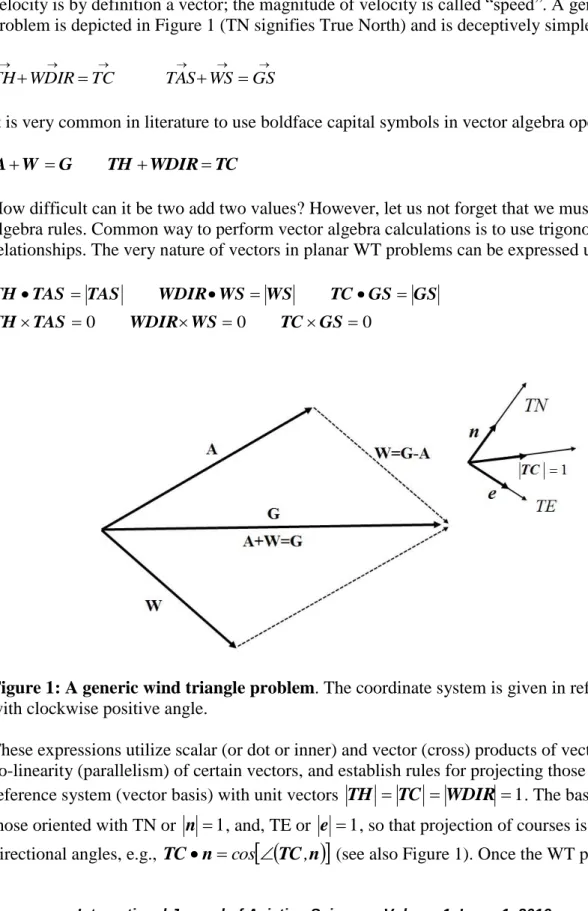
All known and unknown variables used in solving planar WT problems are vectors. For example, velocity is by definition a vector; the magnitude of velocity is called “speed”. A generic WT problem is depicted in Figure 1 (TN signifies True North) and is deceptively simple:
WDIR TC TAS WS GS TH (1)
It is very common in literature to use boldface capital symbols in vector algebra operations.
TC WDIR TH G W A (2)
How difficult can it be two add two values? However, let us not forget that we must obey vector algebra rules. Common way to perform vector algebra calculations is to use trigonometric relationships. The very nature of vectors in planar WT problems can be expressed using
0 0 0 GS TC WS WDIR TAS TH GS GS TC WS WS WDIR TAS TAS TH (3)
Figure 1: A generic wind triangle problem. The coordinate system is given in reference to TN with clockwise positive angle.
These expressions utilize scalar (or dot or inner) and vector (cross) products of vectors, describe co-linearity (parallelism) of certain vectors, and establish rules for projecting those values on any reference system (vector basis) with unit vectors TH TC WDIR 1. The basis vectors are those oriented with TN or n 1, and, TE or e 1, so that projection of courses is given by directional angles, e.g., TCncos
TC,n
(see also Figure 1). Once the WT problem issolved using the TN reference, it is very easily transformed into the Magnetic-North (MN) reference system.
MDEV MH CH MVAR WCA TC MVAR TH MH (4)Here, MVAR stands for the gradually changing magnetic variation based on current terrestrial data and given latitude/longitude information. Magnetic variation will be spatially changing during the flight unless the aircraft continues flying along the “isogonic” (constant-MVAR) line. In the case of the very special isogonic line, i.e. the “agonic” line, the MVAR is zero and
TH=MH and TC=MC. MVAR can be Easterly (E or negative) or Westerly (W or positive). MDEV stands for the Magnetic Deviation of the internal magnetic compass heading (CH), which is caused by the local magnetic fields induced by internal electromagnetic fields (mostly from various NAV/COM radios and GPS units) and is aircraft specific. MDEV can be positive or negative based on the magnetic heading (MH).
There are several ways to solve the WT/DR problems during planning and actual flight phases: 1. Using mechanical (circular) sliding rulers/calculators (such as E-6B, CR-5, CR-2). 2. Using the electronic flight calculator/computer (such as ASA’s CX-2).
3. Deriving trigonometric relationships and programming working equations into them, which will deliver the same result as in item 2 above.
4. Deriving and using approximate relationships, which can also be implemented during the flight phase for quick mental estimation of wind vectors.
We will be mostly concerned with items 3 and 4, and verify the results of computations using the methods described in 1 and 2. A few assumptions and limitations are made here:
The wind vector is designated using WDIR/WS (degrees/knots), and the directional angle WDIR means the azimuth it is coming from.
TC is given in angular degrees and can take any direction in a unit circle.
All speeds used here are in knots, but as long as consistent units are maintained, any other measure can be used such as mph or km/h (kph). There is no theoretical limit to direction and magnitude of wind vector in our considerations. Some TCs will not be possible with some wind vectors. No solution to the WT problem then exists. Both radians and angular degrees are used interchangeably in this text also for the reason of familiarity. The conversion between radians and angular degrees is trivial.
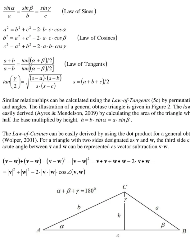
In order to solve the general WT problem one needs to have the same number of equations as there are unknowns. Typically, two equations are needed for two unknowns, while the other four WT parameters must be specified. In order to solve the trigonometric problem illustrated in Figure 1, we use the Law-of-Sines (5a), the Law-of-Cosines (5b), and the Law-of-Tangents (5c) (Ayres and Mendelson, 2009; Bronstein and Semendjajew, 1989; Davies, 2003; Dwight, 1961;
Olza et al., 1974; Spiegel and Liu, 1999; Wolper, 2001; Wylie, 1960):
Lawof Sines
c sin b sin a sin (5a)
Lawof Cosines
2 2 2 2 2 2 2 2 2 2 2 2 cos b a b a c cos c a c a b cos c b c b a (5b)
2 2 Tangents of Law 2 2 c b a s c s s b s a s tan tan tan b a b a (5c)Similar relationships can be calculated using the Law-of-Tangents (5c) by permutation of sides and angles. The illustration of a general obtuse triangle is given in Figure 2. The law-of-sines is easily derived (Ayres & Mendelson, 2009) by calculating the area of the triangle which is one-half the base multiplied by height, hbsinasin.
The Law-of-Cosines can be easily derived by using the dot product for a general obtuse triangle (Wolper, 2001). For a triangle with two sides designated as v and w, the third side closing an acute angle between v and w can be represented as vector subtraction v-w.
v w
w v w v w v w w v v w v w v w v w v , cos 2 2 2 2 2 2 (6)Figure 2:A general obtuse (one angle more than 90°) triangle problem illustrated.
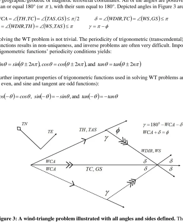
A general WT problem is illustrated in Figure 3. A typical convention is to define air vector (TH, TAS) with one arrow, the ground vector (TC, GS) with two arrows, and the wind vector
solving a trigonometric problem in a frame of reference fixed to the WT and with no relationship to geographic/geodetic or magnetic terrestrial coordinates. All of the angles are positive and less than or equal 180° (or ), with their sum equal to 180°. Depicted angles in Figure 3 are:
TAS , WS TH , WDIR GS , WS TC , WDIR GS , TAS TC , TH WCA 2Solving the WT problem is not trivial. The periodicity of trigonometric (transcendental) functions results in non-uniqueness, and inverse problems are often very difficult. Important trigonometric functions’ periodicity conditions yields:
sin n cos cos n tan tan n
sin 2 , 2 ,and 2
Further important properties of trigonometric functions used in solving WT problems are (cosine is even, and sine and tangent are odd functions):
cos sin
sin tan
tancos , ,and
Figure 3:A wind-triangle problem illustrated with all angles and sides defined. The ambiguity exists with all angles and sides equivalent due to symmetry.
A Taylor series approximation of trigonometric relationships was used (Spiegel & Liu, 1999) for small angles, (in radians). Only the first-order or linear terms have been preserved resulting in the following useful approximations.
! crd ! vers sin ! tan ! cos ! sin 4 0 2 0 6 3 1 2 1 3 3 2 3 1 3 2 3
These approximations are sufficiently good for angles of less than 15°, which is the case in many realistic scenarios, at least regarding the WCA. Wind angles can generally assume any value in unit circle, prohibiting the use of such small-angle approximations of nonlinear trigonometric functions.
It must also be noted that angles in the geographic/geodetic planar coordinate system are counted positive clockwise (starting from TN), while the opposite is true for the angles measured in the unit circle for the trigonometric functions (positive counterclockwise and negative clockwise).
Direct problem I: Unknown GS and TH
The first classical WT problem of dead reckoning that will be solved here has great practical applications in the flight planning phase. A TH and GS are sought that will result in the aircraft maintaining a particular track/course/bearing (e.g., IFR Victor-airway) under given (forecast or reported/measured) steady winds. The GS value is essential for fuel planning and obtainable range as well as planned and actual TOF, which then defines estimated time-of-arrival (ETA) and actual time-of-arrival (ATA). One long flight can be broken into as many legs (segments) as desired and especially so if a change in TC is required. The accuracy of the flight planning phase mostly depends on the fidelity of the wind information.
Using Figure 3 and Equation (5), we utilize the Law-of-Sines to calculate the WCA and TH, and the Law-of-Cosines to compute the GS:
cos WS TAS WS TAS GS TAS sin WS WCA sin 2 2 2 2 (7)The angle between the TC and the WDIR ± 180° is known as the wind-angle . It is the angle between the positive directions of TC and where the WDIR is pointing to (and not coming from as usual) and can be calculated as TC
WDIR180o
. The angle 180o WCA is the angle between the TH and the WDIR180o (see Figure 3). The equation for the dimensionless GS can be now written in dimensionless form:
TAS WS WCA cos TAS GS z 122 (8)We will subsequently see how the non-dimensional ratio WS TAS plays a crucial role in estimating wind effects on cruising aircraft. The solution expressed with Equation (8) is quite general and does not always exist. Finding the general conditions for the existence of a solution of Equation (8) has been conducted, but is beyond the scope of this article due to mathematical
complexity. However, a few important results and conclusions will be presented here. The appearance of a negative sign for zGS TAS simply means that for a general wind intensity the airplane may be flying backward over the ground (GS and TAS have opposite directions).
Theoretically and practically such a solution is possible. However, it is very rare. This is why flying in high (WS/TAS) conditions is impractical and may be very dangerous. Of course, the airplane is never aerodynamically stalled.
We could allow the WCA to be positive (clockwise) for winds coming from the right-of-TC or negative (anti-clockwise) for winds coming from the left-of-TC to calculate the TH. However, that would confuse subsequent calculations and dictate introduction of absolute values of angles. That is why we restrict wind angles to only 0o 180o(from the left or the right of the TC) which may cause ambiguity due to symmetry (Figure 3). The WCA is now:
sin
sin
WCA 1
(9)
Thus, the WCA is always positive (or zero) as sin 0. An additional limitation on the domain of the inverse-sine function (range is
1,1
) is:
2 1 1 1 WCA sin sin (10)This condition implies that some TCs are not possible (or available) when ( 1), and the WT problem has no solution for some fixed TCs. An interesting observation is that when is very large, the available TCs narrow, and in the infinity-limit, the only courses available are into (HW) or with the wind (TW), i.e., when then n where n0,1,2, . The TH is now:
0 2
TC WCA WCA TH (11)The sign ahead of the WCA will be determined based on whether the wind vector is to the right (+) or to the left (-) of the TC in the planar-Earth surface-fixed frame of reference. Several special WT cases exist:
1. Pure headwind (HW) where 180o
and sin 0 (WCA0 and 0). 2. Pure tailwind (TW) where 0o
0 and sin 0 (WCA0 and 180o or ). 3. Pure crosswind (XW) where 90o
2
resulting in sin 1. If we allowed fullcircle angles it would be 270o
3 2
, which is equivalent to 90o
2
, 1
sin , and WCA positive or negative (implying left/right or port/starboard XW). These kind of calculations are easily performed using a circular (trigonometric) slide
trigonometric functions. If the wind vector is coming from the left two quadrants (left HW, XW, or TW) of the TC, the WCA is negative (but designates positive angle in a unit circle) and subtracted from TC. If wind is coming from the right two quadrants, the WCA is positive and is added to TC to obtain TH. In the case of pure HW, the WCA is zero, 180o, 0, the cosine function is positive one (+1), and the groundspeed squared is:
1 2 2 1 z (12)
This results in a familiar case of pure HW: GS = TAS – WS and TH=TC. In the case of pure TW, the WCA is again zero, o
0
, o
180
, the cosine function is negative one (-1), and the groundspeed is. 1 2 2 1 z (13)
This becomes a pure-TW case with GS = TAS + WS and TH=TC. In the case of pure crosswind (XW), the WCA becomes:
60
deg 15 025 1 . WCA sin WCA o Also,cos(90oWCA)sin(WCA)and TASsin(WCA)WS XW , resulting in: 1
1 2
z (14)
Clearly, a fixed TC cannot be maintained with crosswinds XW WSTAS. The TH is as before, TH TCWCA. These are in fact the right-triangle Pythagoras’ rules. The general relationship (Equation 8) reduces to familiar Pythagoras rule in the case of right-triangle kinematics.
Direct problem II: Unknown TC and GS
This direct problem has little use in flight planning or actual flight except in some special cases when calculating drift angles and estimating winds. The geometry of the problem is slightly different as this time the angle between the TH and the WDIR or
WDIR,TH
is known. The known values are wind-vector values WDIR and WS as well as TH and TAS. The angle between the TH and TC is now called drift angle or DA (as opposed to WCA used to maintain a given TC). Using the illustration from Figure 3, and the Law-of-Cosines, we may write (Equation 8) again:
cos
z 1 22 (15)
sin sin DA GS sin WS DA sin 1 (16) The TC is now: DA TH TC (17)When 0 and WCA0, it implies 180o, and one has pure HW with DA equaling zero. The respective GS is then given by Equation (12). When 180o and WCA0, it implies
0
, and we have pure TW with DA equal zero. In that case the GS is given by Equation (13). The solution is very interesting for 90o, in which case the DA will be positive or negative in relationship to the reference system and the GS becomes:
2
1
z (18)
This time there is no restriction on the WS/TAS ratio. This is interesting from the point of view that GSTAS when the wind blows perpendicular to an airplane’s true heading (TH), while
TAS
GS when the wind blows perpendicular to the fixed true course (TC). For very large WS/TAS ratios clearly z, and WCA is zero. This is, of course, such an extreme case with little practical relevance as no aircraft should be flying in such atmospheric conditions and where no route control is possible.
Inverse problem: Unknown winds - WDIR and WS
During actual flight it is very practical to check the wind vector and especially so if the planned TC and GS cannot be maintained with given TH and TAS. For example, modern flight
management systems (FMS) in transport-category (FAR/CS 25) airplanes have the wind vector displayed on the primary flight display (PFD) which is very valuable information. Even smaller, modern, glass-cockpit GA airplanes have the wind-vector displayed on the LCD screen. The triangle laws yield:
GS WCA TAS
WS
WCA sin sin1800 sin (19) ) WCA cos( GS TAS GS TAS WS2 2 2 2 (20)
Knowing TC and TH, the WCA follows immediately, and the WS can be calculated directly. We could then substitute the calculated WS into the Law-of-Sines for this problem and obtain:
11
But this expression for inverse-sine function may introduce ambiguity in the wind angle as the solution is not unique. The other and better way is to obtain the wind angle from the Law-of-Sines incorporating known GS:
WCA sin z sin 1 1 (22)We can decompose the sine function in Equation (22), and after some tedious reductions finally obtain:
WCA cos z WCA sin z tan 1 1 1 1 (23)This is a slightly more complicated expression, but does not need before-hand knowledge of WS and the non-uniqueness of inverse-sine (arcsin) can be resolved better using the inverse-tangent (arctan) function. It is always recommended to use function ATAN2 (such as in Basic, Fortran, Matlab, C++, Excel) as the inverse-tangent function is checked in all four quadrants of the unit circle.
Solving wind triangle problems using complex numbers
Wind triangle problems can be solved more elegantly, avoiding messy trigonometric
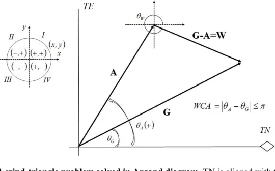
relationships, by using representation of vectors in a complex Cartesian plain (Argand diagrams). A polar or exponential form of vectors is used instead. An illustration of an inverse problem solution is shown in Figure 4. The TN coincides with the x axis or the positive real axis and the counter-clockwise angles are positive as shown in Figure 4.
The air, ground, and wind vectors can be written (Churchill and Brown, 1984; Wylie, 1960) in exponential, trigonometric, polar, and phasor form as:
2 0 1 , , , i WS cis WS sin i cos WS i exp W W GS cis GS sin i cos GS i exp G G TAS cis TAS sin i cos TAS i exp A A W G A W W W W W G G G G G A A A A A (24)Figure 4:A wind-triangle problem solved in Argand diagram. TN is aligned with the positive real axis while TE is aligned with the positive imaginary axis.
The inverse problem can be now described as:
i G A exp
i A W exp
i W exp G W A G (25)Using dot vector products and projecting complex vectors on respective real (X) and imaginary (Y) axis, we obtain:
W W W W G G G G A A A A sin WS Y cos WS X sin GS Y cos GS X sin TAS Y cos TAS X (26)
The intensity, modulus, or absolute value of the wind vector which is WS is now:
2
2 A G A G X Y Y X A G W WS (27)The argument or the counterclockwise angle in a polar vector representation measured from the positive real axis directly resolves an unknown wind angle:
A G A G W X X Y Y tan 1 (28)
regular ATAN trigonometric function delivers ambiguity for the opposing quadrants I and III, and II and IV, and the four-quadrant inverse-tangent function is essential in computing correct angles (see Figure 4).
Let us now solve a practical inverse WT problem of finding the wind vector if the air (A) and ground (G) vectors are fully known (see Figure 4). The data used are TC = 030°, TH = 060°, GS = 120 knots, and TAS = 100 knots. We used our in-house developed WT solvers in True Basic v.6.007 and MS Excel 2013, and obtained rounded WDIR = 153.7° and WS = 60.13 knots. These results were also verified using ASA’s E-6B circular slide rule and ASA’s flight computer CX-2. It must be noted that the computations performed here (Equation 28) result in a wind vector pointing in the direction where the wind is going to, while it is customary in
aviation/aeronautics to use the wind direction where the wind is coming from. So there is 180o change in direction from the calculations performed, i.e., W W . Our calculations have resulted in a wind vector direction of about 333.7°, which is where the wind is pointing to and the inverse direction is about 153.7° (from where wind comes) which is the correct result. Although all calculations are done in 15-significant-digit or double-precision, only two decimal points are used for speed and angle (direction) results.
The mathematics of pure crosswind
A pure crosswind vector (WS = XW) exhibits somewhat curious effects on flying aircraft
maintaining fixed courses (TC). Due to the necessary WCA required to maintain TC, an effective HW component is generated. We will now derive functional relationships and calculate
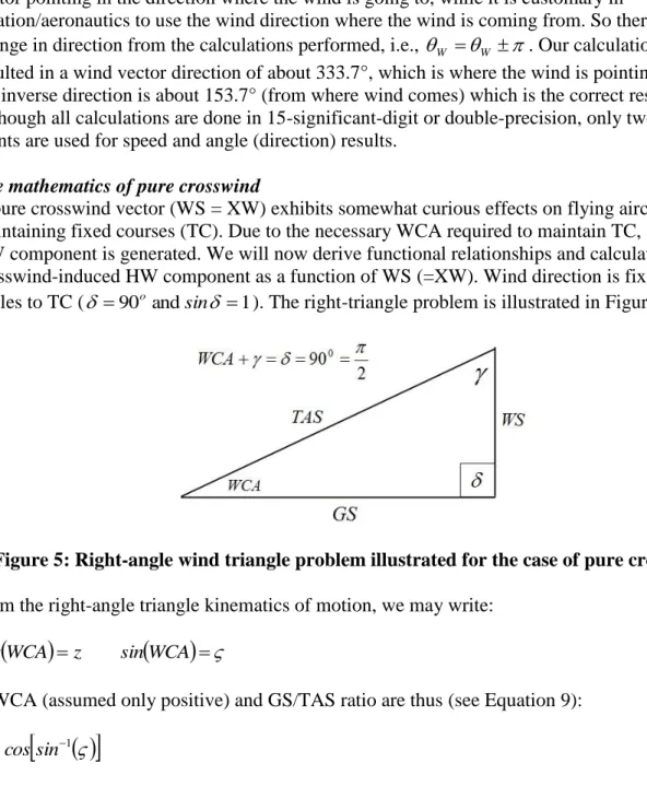
crosswind-induced HW component as a function of WS (=XW). Wind direction is fixed at right angles to TC ( 90oandsin 1). The right-triangle problem is illustrated in Figure 5.
Figure 5:Right-angle wind triangle problem illustrated for the case of pure crosswind. From the right-angle triangle kinematics of motion, we may write:
WCA
z sin
WCA
cos (29)
A WCA (assumed only positive) and GS/TAS ratio are thus (see Equation 9):
1
cossin
The induced HW component due to XW is thus:
0 1 1 1 sin cos z TAS HW ind (31)The non-dimensional GS is now:
1z (32)
Where crosswind function is defined in terms of versed sine of WCA:
cos
sin
cos
WCA
vers
WCA
1
1 1
(33)
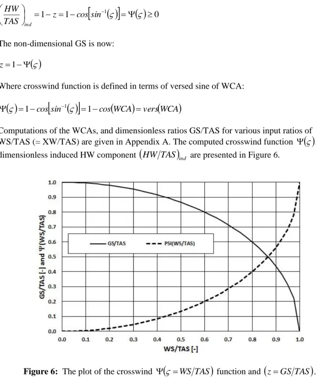
Computations of the WCAs, and dimensionless ratios GS/TAS for various input ratios of
WS/TAS (= XW/TAS) are given in Appendix A. The computed crosswind function
, or the dimensionless induced HW component
HW TAS
ind are presented in Figure 6.Figure 6: The plot of the crosswind
WS TAS
function and
zGS TAS
.The effective headwind component
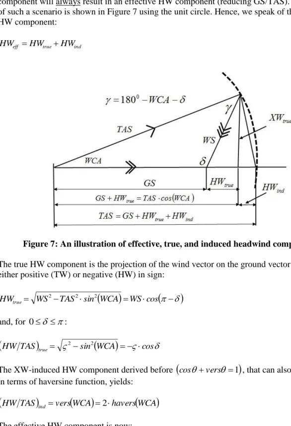
Previous considerations have shown that a XW component will create an induced HW
component. The general wind vector when decomposed into two projections, one parallel and one perpendicular to the TC, will also have a true HW (or TW) component based on its
projection on TC. While wind projection on the TC can result in a true TW or HW, the XW component will always result in an effective HW component (reducing GS/TAS). An illustration of such a scenario is shown in Figure 7 using the unit circle. Hence, we speak of the effective HW component:
ind true
eff HW HW
HW (34)
Figure 7: An illustration of effective, true, and induced headwind components.
The true HW component is the projection of the wind vector on the ground vector and can be either positive (TW) or negative (HW) in sign:
WS TAS sin WCA WS cos HWtrue 2 2 2 (35) and, for 0 :
HW TAS
true 2sin2
WCA
cos (36) The XW-induced HW component derived before
cosvers 1
, that can also be expressed in terms of haversine function, yields:
HW TAS
ind vers
WCA
2havers
WCA
(37)
WCA
sin
WCA
vers TAS HW TAS HW TAS HW true ind eff 2 2 (38)The non-dimensional speed ratiozis (0 ):
sin sin
cos cosz 1 (39)
This is the most general equation which gives GS as a function of an arbitrary wind vector for a given course and with sin 1. In the case of pure XW or 2, this is the familiar result (Equation 30), zcos
sin1
for 1.The induced headwind component due to WCA will only exist for the aircraft in free flight. During takeoff and landing operations, an airplane will be only experiencing true
headwind/tailwind components, and the crosswind will be compensated for by the friction between the landing gear and runway surface. In the case of pure HW ( ) and pure TW ( 0) these are familiar expressions, zHW 1 andzTW 1, respectively.
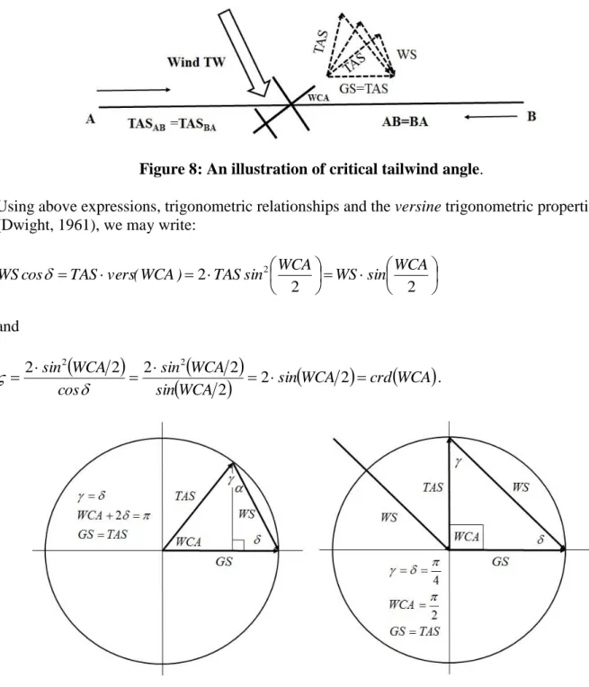
The critical tailwind angle
Headwinds always reduce GS, and tailwinds should apparently always increase GS. This seems logical, but as we will see, even TWs can reduce GS. As previous considerations have shown, the XW-component of a general wind vector will always reduce GS so that z1. On the other side the true TW component (projection onto and in a direction of TC) of the general TW will increase GS, HWind TWtrue, when critical angle and HWind TWtrue, implies, GSTAS.
The angle at which a general TW acts will depend on the ratio for z1. An illustration of an airplane maintaining track under various TWs for which the induced HW component neutralizes true TW component is shown in Figure 8. Looking at the isosceles wind-triangle shown in Figure 9, we can write for TW component (0 2):
TAS cos WS ) WCA cos( TAS GS (40)
This relationship comes directly from Equation 39. Due to the familiar properties of isosceles triangles (equilateral triangle is a special case with all three sides equal and every angle being 60°), we can write: 2 2 2 2 WCA WCA WCA
Figure 8:An illustration of critical tailwind angle.
Using above expressions, trigonometric relationships and the versine trigonometric properties (Dwight, 1961), we may write:
2 2
2 TASsin2 WCA WS sin WCA ) WCA ( vers TAS cos WS (41) and
sin
WCA
crd
WCA
WCA sin WCA sin cos WCA sin 2 2 2 2 2 2 2 2 2 . (42)Figure 9:Critical tailwind angle and the solution of isosceles triangle.
The old and somewhat obsolete trigonometric functions versine (vers), haversine (havers), and
chord (crd) directly describe the WS vector of the isosceles triangle (Figure 9). The archaic function chord was known to and used by the famous Greek-Egyptian astronomer Claudius Ptolemaeus, or Ptolemy (AD 100-170) (Sinnott, 1984; Toomer, 1970). The haversine function is very important in calculating Orthodromes on the spherical Earth and especially for calculating
small angular separation of astronomical objects (Sinnott, 1984). The critical WCA angle is thus:
2 2 1 sin
WCA* (43)
And the critical TW angle at which GS = TAS or z1is:
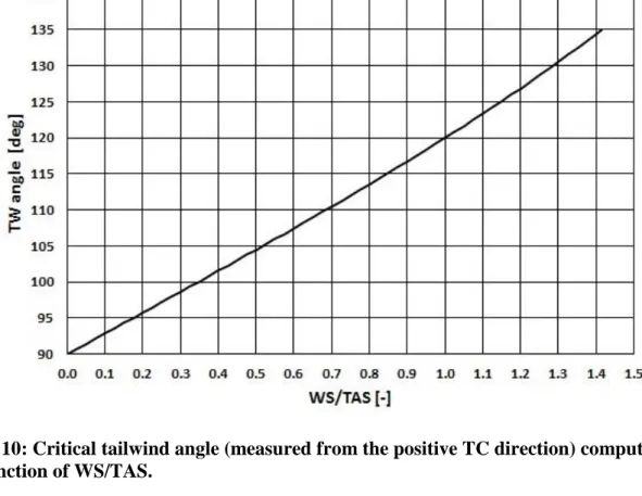
2 2 2 2 2 2 1 1 sin sin WCA * * * * (44)The critical tailwind angle computations are presented in Figure 10. For a special case when WS = TAS = GS or z1, we have equilateral triangle and the critical angle is:
o * sin 1 2 2 6 3 60 2 1 The critical wind angle measured from the positive direction of TC is then * * 120o. Another special case scenario is for WCA = 90°. In that case the TAS and GS vectors are perpendicular and the entire TAS is used only to compensate for pure XW (resulting in GS = 0 along the TC), while the true TW component actually contributes to the entire GS:
o * * o * * WCA 135 4 3 45 4 4 2 2 2
In this case, the inverse critical TW problem will result in 2sin
2*
1.414. The significance of this considerations is that tailwinds may exist in cruise, but in some cases, the true TW component (projected along and in a direction of TC) is being canceled by the reduced GS due to the WCA required to maintain the TC, i.e, induced HW component. For example, an aircraft cruising at 100 KTAS will have to fly perpendicular to its TC just to offset the XW component of a 141 knot tailwind WS coming from the relative angle of 135° of its nose or 45° of its tail. The GS is 100 knots. In this particular case WS/TAS is about 1.414 (i.e., 2 ) and tailwind blowing at angles between 90° and 135° measured from the TC direction will actually result in reduced GS or z1.Figure 10:Critical tailwind angle (measured from the positive TC direction) computations as a function of WS/TAS.
The effect of atmospheric wind on TOF
On round-robin (closed loop) flights, any steady wind vector (constant WDIR and WS) will always reduce average ground-speed and increase TOF. The TOF for a general multi-segment trajectory can be defined as:
w eff N i i N i i w,i i L w HW v , TAS v t v v s s v s v ds TOF
0 (45)In theory, the TAS and the effective HW/TW can change as a function of time or as a function of trajectory path. To mathematically show a simple case of how TOF always increases with the constant wind vector, we will take a straight distance flight departing point A toward point B at given distance with return back to A. The total distance (A-B-A) is thus twice the distance A-B (A-B=B-A). Let us assume that TAS does not change in flight, yielding a hyperbolic
relationship: ____ BA AB BA AB BA BA AB AB BA AB GS L GS GS GS GS L GS L GS L T T T 2 (46)
Spiegel and Liu, 1999) of the forward and return legs: TAS GS GS GS GS GS GS GS L L L BA AB BA AB BA AB ____ BA AB 1 1 2 2 (47)
Clearly, if any of the two GS’s is zero so is the average GS, and TOF becomes infinite. One must be careful not to use arithmetic averages when calculating time-speed-distance problems, but harmonic averages instead.
TOF can be now expressed in terms of known TAS and effective headwind/tailwind component (taking into account true and XW-induced wind components). Since the WDIR and WS are assumed constant and the induced HW component always reduces GS, we may write using Equations (46) and (47):
ind true
ind
true
true ind true ind HW HW TAS HW HW TAS HW HW TAS HW HW TAS L T 2 2 (48)
After lengthy reductions, we obtain:
2 2 1 1 2 true ind ind HW NW HW NW ABA t TAS HW TAS HW TAS HW TAS L T T T dt
(49)For relatively small XW-induced HW components (WCA less than about 12 degrees or 2
0. TAS
XW ), which is common in jet airplane operations, we may utilize true HW
component only. In the case of true HW only or induced HW component only, respective time-factors yield:
ind
ind
HW true true HW 1 1 HW TAS 1 1 HW TAS 2 (50)It is easy to see in the limit from Equation (49) that when the induced component is zero and the true component is one, the wind factor is infinite. The same holds if the induced component is one and the true is zero, but the rate of increase of the rate-factor is slower (Equation 50).
Clearly, the TNW is no-wind TOF, while the effective wind coefficient is always, HW 1. In the limit:
HW TAS
x T lim lim ABA x HW x1 1 We would get similar results if only the induced component exists or if both components add to one. This is the proof that whenever an approximately constant wind vector exists on closed-loop
flights it will always result in increased TOF. That is, any steady wind vector will actually act as an effective HW on round-robin flights, although in any individual leg it may actually act as pure TW. The negative effect of HW is thus stronger than the positive effect of TW, a fact well
known, but apparently not quite understood. The primary reason is that HW not only reduces GS, but also prolongs exposure to it. The average GS with mostly true HW component is now:
1 HW TAS 2
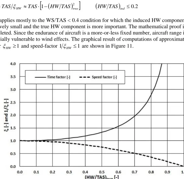
HW TAS
0.2 TAS TAS GS HW true ind ____ (51)This applies mostly to the WS/TAS < 0.4 condition for which the induced HW component is still relatively small and the true HW component is more important. The mathematical proof is now completed. Since the endurance of aircraft is a more-or-less fixed number, aircraft range is especially vulnerable to wind effects. The graphical result of computations of approximate time-factor HW 1 and speed-factor 1HW 1 are shown in Figure 11.
Figure 11:The effect of steady true headwind on time of flight and average speed of multi-leg closed flights (round-robin).
The results presented in Figure 11 and Equations (49), (50), and (51) are of utmost importance in flight operations. TOF increases first slowly and then rapidly with the true HW/TAS (Equation 50), and the GS decreases quadratically (Equation 51) with the increased true HW-component. The increase of TOF with the increased true HW component can be described as:
ABA
true x ABA TAS HW x T lim x x TAS L dt T 1 2 2 1 2 2Similarly, for the pure induced HW component, the TOF would increase without bound, but a bit slower than for the case of true HW component. It is easy to show that for small WCAs the effective wind is mostly in true HW component. In the general case of the closed multi-leg flight trajectory, we may write:
n i i i NW n i i i n i i TAS L T GS L T T 1 1 1The influence of effective wind on PET, PNR, and ROA
The PET value is an aircraft-specific scenario signifying emergency situation in which the decision must be made to return to departure (or previous adequate airport) or proceed to destination or next enroute alternate airport. PET has special importance in ETOPS operations (FAA, 2008) in the case where the airplane crew must decide to return to a previous point or continue on to the next. With ETOPS an airplane must always be within given flying time (e.g., 180/207 minutes) from an adequate airport in the case of engine shutdown/failure and reduced TAS, which will also imply drift-down to lower cruising altitudes. The concept of ETOPS (FAA, 2008) is based on the correct determination of PET location and TOF. On the other hand, the PNR, also known as the point-of-safe-return, signifies an airport emergency situation, in which case the aircraft still can return to its departure point. Radius-of-action (ROA) is closely related to PNR, so it will not be considered separately. All conclusions from PNR considerations can be directly applied to ROA. Numerical calculations of PNR and PET in airline operations are, for example, described in Filippone (2012). Understanding and forecasting wind vectors is crucial in aircraft performance and operations (Daidzic, 2014; Hale and Steiger, 1979; Hale, 1984;
Filippone, 2006, 2012).
The expression for PET is calculated knowing the distance between the point A (departure) and B (destination) and given TAS while the effective HW will be constant for forward and return flight (TPETA TPETB):
ind true AB fwd ret ret AB PET TAS HW TAS HW L GS GS GS L L 1 1 2 (52)Using the definition of the WCA (Equation 9), we may finally write:
1 1 2 1 1 sin sin cos cos L L AB PET (53)which acts equally in reducing GS in both legs and does not affect the PET location. Otherwise, the PET will always move into the direction from which the true wind-component comes:
HW 0,XW 0
2
2 2 0 XW , 0 HW 0 2 0 XW , 0 HW true true true AB PET AB PET AB PET L L L L L L The PNR can be written for a similar problem when flying from A to B on a straight course with constant effective wind. The effective endurance is the amount of flying time not counting fuel reserves and normally applies only at a given TAS, altitude, specific-fuel-consumption (SFC), and known initial fuel amount. Since the flight is round-robin the wind will always reduce the range of the aircraft and increase flight time compared to a no-wind situation:
HW eff ret fwd fwd ret eff PNR TAS E GS GS GS GS E L 2 (54)
The product (EeffTAS 2) is the maximum no-wind half-range or the maximum distance the aircraft can fly outbound and still be able to return with zero wind to its destination. This is equivalent to the ROA definition. The existence of wind always results in effective HW in round-robin flights with given fixed courses. Unlike PET, which implies aircraft emergency, the PNR signifies airport emergency. The ROA can be similarly defined as:
Max fuelRes Mission
HWROA E E E TAS
L
2 1
(55)
In the end it is instructive to estimate the ratio of PET and PNR distances. Using Equations (52) and (53), we may write:
1 fwd min fwd fwd eff PET PNR PET GS GS GS E L L L (56)The PET is located typically halfway between two airports and always moves into the wind, while the PNR distance can be significantly longer than PNR. The significance of GS in the nominator is that this is the minimum GS allowed to reach destination.
Small-perturbation theory of wind effects
An important question arises as to how small changes in wind vector (direction and/or speed measurements) affect air and ground vectors. This consideration is important from the aspect of track/route optimization and sensitivity to winds. Additionally, wind vector measurements are susceptible to smaller or larger experimental and instrumentation uncertainties. Therefore, we have developed a theory based on the small (linear) perturbation of the wind vector to estimate
changes in WCA and GS for a given fixed TC. Other WT problems could also be easily derived following the same strategy as applied below. Typically, first-order linear perturbation analysis of nonlinear functional relationships is valid only for small changes of an independent value up to about 10-15% and becomes increasingly inaccurate for larger changes. Using the fact that
,f
WCA ,z g
, , and using Equations (8) and (9), we obtain for total differentials (Ayres and Mendelson, 2009; Spiegel and Liu, 1999):
WCA f f z g g (57)Evaluating partial derivatives from Equations (8) and (9) and replacing them in Equation (55), one obtains after tedious mathematical reduction (for WCAsin1
sin
0):
0 1 0 1 0 2 1 1 sin sin cos sin sin sin sin WCA WCA (58) and
WCA WCA y sin WCA y sin y cos z z 0 0 0 2 (59)Here, we designatedy12 2 cos 0, and used the fact that the three internal WT angles satisfy d d
WCA
d 0and WCA (must be in radians). The meaning of terms in small perturbations is very clear. In Equation (58), the first term shows the relative change in WCA due to the small relative change of wind speed magnitude, while the second term shows the WCA change due to the small perturbed value of wind angle. Interestingly, Equation (59) has three terms affecting the change of GS. The first is due to the change of windspeed (WS) alone, the second due to change of wind (true wind component) and the third caused by the change in WCA, which is nothing else, but the induced wind component due to the fact that TC must be fixed and is evaluated first with Equation (58). In the case when the wind vector is aligned with the ground (and thus also air) vector, only the first term in Equation (59) remains. The subscript “0” simply means that the set point is calculated at known equilibrium (steady-state) position and the perturbations are added to it. Singularities exist when WCA0, for 0 or , or 0 or .Results and Discussion
The first result presented will be the solution of the direct problem. The graphical result of the wind-triangle problem is depicted in Figure 12 with the values of known and computed figures shown. We used a MS Excel 2013 spreadsheet program for computations and graphical
presentation. The results of computations were also verified using the structured high-level programming language True Basic v.6.007. The results and illustration of the inverse WT problem using complex numbers and polar/exponential wind vector representation is shown in Figure 13. It must be said that solutions involving complex analysis are far more elegant and simpler than tedious and cumbersome traditional trigonometric calculations.
The WCA is a function of WS/TAS ratio and the WDIR angle on the fixed TC using the equation derived earlier (Equation 9). The results of WCA calculations are presented in Figure 14. At 1, the WCA must be equal to the angle of wind for the fixed TC. This is logical as the airplane must turn completely into the HW if it is to maintain course, but the GS will be then zero, i.e.,
z
0
. The next result is the computation of the zGS TAS ratio as a function of angles , , and dimensionless wind speed WS TAS as illustrated in Figure 15.Figure 12:Solution of the direct wind triangle problem using trigonometric WT relationships.
In the case of z1, which results in the critical TW* angle, a following transcendental equation must be solved for unknown critical TW* angle:
2
02
2
cos cos (60)
The solution for 0 is trivial. The other solution for the critical angle is obtained from:
2 cos1
2cos * * (61)
Figure 13:Solution of inverse wind triangle problem using complex representation of air, ground, and wind vectors.
2
2 2 2 2 1 1 cos sin WCA* * (62) and
2 2 1 2 * * * WCA crd WCA sin cos .This is the identical result we obtained previously from direct critical TW angle considerations. It is somewhat surprising and unexpected that such a critical TW angle was never mentioned before in any publically available literature or academic/scientific article to the best of our knowledge.
Figure 14:Wind correction angle calculations.
A movement of the z1 point to the left (increasing TW angles) is evident from Figure 15. Also the behavior of the 1 curve is very interesting. It crosses the z1 line at 60° and hits zero GS at 90° as expected. After that, it remains constantly at zero. An aircraft must turn directly into the wind if it is to maintain TC, which is somewhat irrelevant as the GS will be zero. The GSs between 60° and 90° of the tail will result in GSTAS. For the case when 1, there will be a
“forbidden region” of wind angles where sin 1 and for which it is impossible for an aircraft to maintain fixed TC. The “allowed zone” of courses will be an ever sharper cone and in the limit of 1, the only possible course is the direction of the wind (into wind or with it). Additionally, for 1, a region z0 exists, implying that the GS vector will be opposite of the TAS vector as evident in Figure 15. Flight under such conditions makes little practical sense, but is possible yet unsafe.
Surprisingly, some electronic flight computers tested, such as ASA’s CX-2 will not report an error condition when trying to solve the impossible WT problem (TC restriction with 1), but will instead just return the original TC and TAS as a TH and GS. The mechanical circular slide computers, such as Jeppesen’s E-6B or CR-2, ASA’s E6-B, or Pooley’s CRP-5, will not be able, in general, to solve WT problems for large ratios. Granted it would be highly unwise to attempt to fly in high WS/TAS conditions, nevertheless the clear restrictions and limits are never spelled out in flight computer (electronic or mechanical) operating manuals nor taught to flying students and practitioners.
Figure 15:(GS/TAS) calculations as a function of (WS/TAS) and wind angle measured of the tail. Pure TW is at 0° and pure HW is at 180°.