Adaptive dynamic programming-based controller with admittance adaptation for robot–environment interaction

Adaptive dynamic programming-based

controller with admittance adaptation

for robot–environment interaction

Hong Zhan

, Dianye Huang

, Zhaopeng Chen

, Min Wang

and

Chenguang Yang

Abstract

The problem of optimal tracking control for robot–environment interaction is studied in this article. The environment is regarded as a linear system and an admittance control with iterative linear quadratic regulator method is obtained to guarantee the compliant behaviour. Meanwhile, an adaptive dynamic programming-based controller is proposed. Under adaptive dynamic programming frame, the critic network is performed with radial basis function neural network to approximate the optimal cost, and the neural network weight updating law is incorporated with an additional stabilizing term to eliminate the requirement for the initial admissible control. The stability of the system is proved by Lyapunov theorem. The simulation results demonstrate the effectiveness of the proposed control scheme.

Keywords

Adaptive dynamic programming, admittance adaptation, neural network, optimal control, robot–environment interaction

Date received: 17 July 2019; accepted: 7 April 2020 Topic: Robot Manipulation and Control

Topic Editor: Lino Marques Associate Editor: Jian Huang

Introduction

Robot applications are becoming more and more wide-spread, such as rehabilitation therapy, assembly automation and surgery.1–4 They can either work independently to accomplish tasks or cooperate with their human partners for certain tasks. In the actual application process, the robot will inevitably interact with the external environments.5–7 Consequently, in recent years, interaction control between the robot and environment has attracted great concern and is considered to be greatly important.

In existing research, two main approaches are applied to achieve compliant behaviour of the robot, that is, hybrid position/force control and impedance control.8,9 The first approach requires the position subspace and force subspace decomposition, task planning and control law switching in the execution process. Without considering the dynamic coupling of the environment and the robot, the accuracy

of the hybrid position/force control cannot be guaranteed.10 In contrast, the second approach aims to adjust the mechan-ical impedance to a target one, which will guarantee the robot to be complaint with the interaction force imposed by the external environment. Impedance control ensures the safety of the robot and the environment and it has been

1

Key Lab of Autonomous Systems and Networked Control, Ministry of Education, School of Automation Science and Engineering, South China University of Technology, Guangzhou, China

2_{TAMS Group, Department of Informatics, University of Hamburg,}

Hamburg, D22527 Hamburg, Germany

3_{Bristol Robotics Laboratory, University of the West of England, Bristol,}

UK

Corresponding author:

Chenguang Yang, Bristol Robotics Laboratory, University of the West of England, Bristol BS16 1QY, UK.

Email: [email protected]

International Journal of Advanced Robotic Systems

May-June 2020: 1–11

ªThe Author(s) 2020 Article reuse guidelines: sagepub.com/journals-permissions DOI: 10.1177/1729881420924610 journals.sagepub.com/home/arx

Creative Commons CC BY: This article is distributed under the terms of the Creative Commons Attribution 4.0 License (https://creativecommons.org/licenses/by/4.0/) which permits any use, reproduction and distribution of the work without further permission provided the original work is attributed as specified on the SAGE and Open Access pages (https://us.sagepub.com/en-us/nam/ open-access-at-sage).

proved to be more feasible and has better robustness. According to the causality of the controller, impedance control has two implementation methods, one is named impedance control and the other is admittance control. In impedance control system, the interaction force can be estimated from the desired motion trajectory and impe-dance model, while in admittance control system, the ref-erence trajectory is obtained from the measured environmental external force and the desired admittance model. Therefore, in this article, admittance control is adopted to solve the problem of robot–environment inter-action control.

In admittance control system, force and the admittance model are two important parts. When robot–environment interaction exists, the force can be detected and measured by the sensors installed on the end-effector of the robot arm. But, how to derive optimal parameters of the admittance model is non-trivial. On the one hand, it is usually difficult to derive the desired admittance model because of the com-plexity of environmental dynamics; on the other hand, a fixed admittance model cannot satisfy all cases. Taking human–robot cooperation as an example, variable admit-tance control is necessary to ensure more efficient perfor-mance.11 To solve these problems, iterative learning has been studied in robot intelligent control area. It has been investigated to obtain admittance parameters to adapt to unknown environment. The aim of this approach is to intro-duce human learning skills into the robot and improve con-trol performance by repeating a task. Cohen and Flash12 proposed an impedance learning control scheme using an associative search network to complete a wall-following work. Neural network (NN) is introduced into the impedance control to regulate the parameters.13However, the iterative learning method requires the robot to operate repeatedly, which brings inconvenience in practical process and is not feasible in many situations. Love and Book,14Uemura and Kawamura,15 Gribovskaya et al.,16 Stanisic and Fern´an-dez,17Landi et al.18and Yao et al.19have proposed to utilize adaptation approaches to address the problems stated above. Robotic motion control is a challenging task as it is difficult to obtain accurate model concerning that the robot is a non-linear and highly coupled system. Proportional– integral–derivative (PID) control, NN control, adaptive control and other control methods have been applied to the robot system.20–27As a classical control method, PID con-trol is employed to the robot system and can track the given reference trajectory well.28 It is acknowledged that PID control has some advantages, such as simple structure and good robustness, but it is not easy to select suitable PID parameters if the controlled plant is complex. In addition, when dynamic uncertainties exist in the system, PID con-trol cannot satisfy the performance requirements for the magnitude of overshoot, the rising and settling time and so on. NN has the fundamental characteristics of human brain and can simulate human behaviour for information processing, therefore it is widely used in the control field

for unknown system identification. NN control can model the uncertain dynamics online to improve the system per-formance.29An admittance adaptation method and the NN-based controller are applied into the robot system.30

Tracking control is a significant research issue in the domain of robot intelligent control. For a controlled sys-tem, stability is just the minimum requirement. Optimal control needs to be considered, that is, it is required to design an optimal tracking controller, which could ensure system stability of the robot while minimizing the cost function. Werbos31 proposed adaptive dynamic program-ming (ADP) strategy and it is considered to be an effective approach to resolve the optimal control problem.32The key of ADP method is to find a solution of Hamilton–Jacobi– Bellman (HJB) equation. However, because it is a partial differential equation, when the controlled system is non-linear but not non-linear, its analytical solution will be very difficult to obtain, or even impossible. To solve the above problem, policy iterative is considered as an effective method to find the approximate solution, which requires initial stability control.33However, in practical process, the initial admissible control is usually very difficult to satisfy. Then, NN is introduced to derive an approximate solution of the HJB equation. The approximate solution is obtained by NN-based method, meanwhile the requirement of initial stability is eliminated with the incorporation of an addi-tional term.34,35

Yang et al.30 paid attention to the robot–environment interaction control, but did not consider the optimization problem. However, for the robot, how to perform path tracking optimization and minimize the cost function is very important. Based on the above discussion, the optimal tracking control problem for robot–environment interaction is studied in this article. Moreover, the admittance control and ADP approach are adopted to improve the system per-formance. The contributions of this article are listed below: 1. The environment with unknown dynamics is mod-elled as a linear system. An admittance adaptation method with iterative linear–quadratic regulator (LQR) is obtained to achieve a compliant behaviour.

2. ADP approach is introduced into the robot system to solve the optimal tracking problem. The critic net-work with radial basis function (RBF) is developed to approximate the minimum cost function. In addi-tion, to eliminate the requirement for initial admis-sible control, a stabilizing term is incorporated into NN weight updating law.

The rest of this article is arranged as follows. Firstly, the robot and environment systems and control objectives are described. Next, the control scheme including admittance adaptation and optimal control using ADP is developed. Then, simulation studies are given. Finally, the conclusion is drawn.

Preliminaries and problem formulation

Robot dynamics

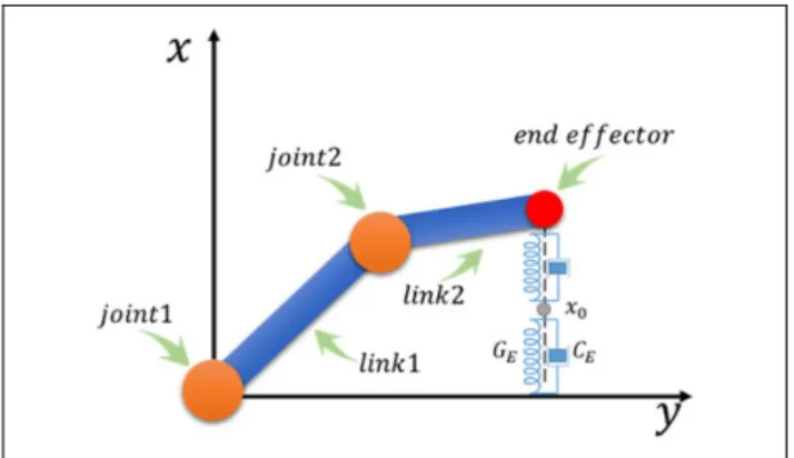
The n-link robot manipulator dynamics is showed as the following Lagrangian form

MðqÞ€qþCðq;q_Þq_þGðqÞ ¼ ð1Þ

where q¼ ½q₁;q₂;. . .;q_nT2Rn_{, q_ ¼ ½q_}

1;q_2;. . .;q_n

T₂

Rn_{and€q¼ ½€q}

1;€q2;. . .;€qnT2Rnrepresent the robot

posi-tion vector, velocity vector and acceleraposi-tion vector in joint space, respectively. 2Rn _{is the joint torque,}

while MðqÞ 2Rnn_{, Cðq;q_Þ 2R}nn _{and GðqÞ 2R}n _are

known matrices and denote the inertial matrix, Corio-lis/centrifugal matrix and gravity vector, respectively. For convenience,M,CandGdenote the known matrices MðqÞ, Cðq;q_Þ and GðqÞ in the following section, respectively.

Define the reference trajectory asq_r2Rn_{, and the}

track-ing errorq_e2Rn_{is shown as follows}

q_e¼qq_r ð2Þ

Then, the first and second time derivative ofqeare given

below

_

q_e ¼q_q__r €

q_e ¼€q€q_r ð3Þ

We define the sliding motion surfacexas follows x¼Lqeþq_e ð4Þ

whereL2Rnnis a constant positive matrix. According to equations (2) to (4), we can get

_

q¼ xLq_eþq__r €

q¼ x_Lq_eþ€q_r ð5Þ Substituting equation (5) into equation (1), the error dynamics is obtained as follows

_

x¼ M1_CðxLq

eþq_rÞ M1G

€qrþLq_eþM1

ð6Þ

Then, the following system is obtained

_

x¼fðxÞ þgðxÞ ð7Þ

The non-linear functions f :Rn!Rn and g:Rn!

Rnn_{in equation (7) are specified by}

fðxÞ ¼ M1_CðxLq

eþq_rÞ M1G€qrþLq_e

gðxÞ ¼M1 ð8Þ

Environment dynamics

It is assumed that the dynamics of environmental interac-tion force subject to the equainterac-tion given below

CEx_þGEx¼ F ð9Þ

where CE and GE represent the unknown damping and

stiffness of the environment, respectively.F denotes the interaction force and can be detected and measured by a force sensor. xis the end-effector position in Cartesian space and the corresponding desired trajectory xd is

defined as

_

xd ¼Udxd ð10Þ

where U2Rmm _{is a known matrix. Subsequently, we}

define h¼ ½x;xdT. Thus, combining equation (9) with

equation (10), dynamics of the unknown environment and the desired trajectory are generated by

_ h¼ C 1 E GE 0 0 Ud " # hþ C 1 E 0 " # F ¼AehþBeF ð11Þ

If we take equation (11) as a linear system withFas its control input andhas its states to be controlled, this equa-tion relatesxwithxdvia the optimal feedback control law

F¼ Kehwhose aim is to minimize the cost function

G1¼ ð1 0 x_eTQ_E1xeþFTREF dt ð12Þ

This cost function also indicates that our motivation of modifying a desired trajectoryxdis to balance the contact

forceFwith the tracking errorxe¼:xxd. And this

bal-ance can be tuned via the user-definedQ_E1andRE.

In this section, the robot and environment dynamics are modelled. Then, we will design a control strategy to achieve the compliant behaviour and optimal tracking con-trol in case the robot interacts with the environment.

Control scheme

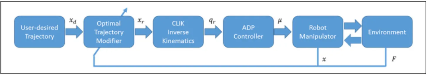
A control scheme consisting of three parts as shown in Figure 1 including an optimal trajectory modifier using admittance control, a closed-loop inverse kinematics (CLIK) solver and a trajectory tracking controller based on ADP technique is designed in this section.

Trajectory modification using admittance control

The solution to equation (12) is an analogy with the LQR problem. It can be rewritten as

G ¼ ð1 0 hT_Q EhþFTREF dt Q_E ¼ QE1 QE1Ud U_dTQ_E1 UT_dQ_E1Ud " # _ð13Þ

whose system counterpart is consistent with equation (11). In this subsection, an algorithm proposed by Jiang and Jiang36is adopted to solve the algebraic Riccati equation (ARE) in equation (14) with unknown environment para-metersCE,GEto derive the feedback gainKe

PAeþAeTPþQEPBeRE1BeTP¼0

Ke¼ RE1BeTP

ð14Þ

Some notations are outlined here. n, m andd are the length of h,Fand the sample times integer, respectively. The sampled signal together with the historical ones com-prising the matrix as follows

^ p ¼½p₁₁;2p₁₂;. . .;2p_1n;p₂₂;2p₂₃;. . .;p_nnT h¼ h2 1;h1h2;. . .;h1hn;h22;h2h3;. . .;hn2 T dh¼½hð Þ t1 hð Þt0 ;hð Þ t2 hð Þt1 ;. . .;hð Þ td hðtd1ÞT Ih_h¼ ðt1 t0 hhdt; ðt2 t1 hhdt;. . .; ðtd td1 hhdt T Ih_F ¼ ðt1 t0 hf dt; ðt2 t1 hFdt;. . .; ðtd td1 hFdt T ð15Þ where p2R12nðnþ1Þ, h2R12nðn1Þ, dh2Rd12nðn1Þ, Ih h2 Rdn2

,Ih_F 2Rdnm_{andstand for the Kronecker product,}

andp_ijandh_idenote entries ofPandh, respectively rankhIh_h;Ih_Fi ¼nðnþ1Þ

2 þnm ð16Þ When the number of sampled data is large enough and the rank condition in equation (16) is satisfied, the algorithm can solve Ke by iteratively calculating

equa-tion (17) until ^pðkÞ converge to an acceptable range e, that is, jjp^ðkÞ^pðk1Þjj<e with k k denoting the 2-norm of Q_EðkÞ¼Q_EþK_eðkÞTREKðekÞ YðkÞ¼ dh;2Ih h InKðekÞTRE 2Ih_FðInREÞ h i XðkÞ¼ Ih_hvecQð_EkÞ ^ pðkÞ vec Kðkþ1Þ e " # ¼YðkÞTYðkÞ1YðkÞTXðkÞ ð17Þ

where the superscriptðkÞdenotes the index of the iteration, vecðÞ denotes the column vectorization of and In2Rnnis an identity matrix.

Once the optimal feedback gainKeis obtained, we can

use it to modifyxd. Formulations are given as below

F¼ Keh¼ ½Ke1 Ke2

x xd

ð18Þ

whereKe1andKe2are compatible matrix fromKe. Finally,

the modified trajectoryxrto be tracked is calculated, which

is equivalent to thexin equation (18)

xr ¼ Ke11FKe11Ke2xd ð19Þ

Inverse kinematics using CLIK

The CLIK algorithm is employed to resolve the Cartesian reference trajectoryxrinto the oneqrin joint space.37Let

the solution errore:¼kðq_rÞ xr wherekðÞdenotes the

forward kinematics andeis given by

_

e¼ Kfe ð20Þ

whereKfis a positive user-defined matrix that decides the

convergent rate of e. Expanding the above equations and combining withx_¼Jcoq_andJco¼@kðqÞ=@q, the

follow-ing equation holds

_

qr¼Jycoðx_rKfðkðqrÞ xrÞÞ ð21Þ

integrating of which yields the CLIK method q_r ¼ ðt 0 Jyx_rJycoKfðkðqrÞ xrÞ dt ð22Þ whereqð0Þ ¼k1ðxrð0ÞÞ,Jyco¼JTco JcoJTcoþsIn 1 , and s2Ris introduced to avoid the singularity problem which is recommended to be assigned small enough for improving the solution accuracy.

Optimal control using ADP

As mentioned in the Introduction section, it is very impor-tant to optimize the trajectory tracking while minimizing the design cost for robots. On the basis of optimal theory, the optimal control of the system (7) can be derived by solving the HJB equation in the frame of ADP. Conse-quently, in this subsection, our target is to find such an optimal control.

Assume that the functionsfðxÞandgðxÞare Lipschitz continuous inR2n and system (7) is controllable, then the optimal controlshould minimize the cost function which is expressed as

JðxðtÞÞ ¼ ð1 t FðxðtÞÞ þUðxðtÞ; ðxðtÞÞÞ ½ dt ð23Þ where FðxðtÞÞ ¼xðtÞTQxðtÞ, UðxðtÞ; ðxðtÞÞÞ ¼

ðxðtÞÞTRðxðtÞÞ,Q2Rnn_andR2Rnn_{are symmetric}

positive definite matrices. For robot system (7), the opti-mal controlshould not only guarantee system stability but also can make the cost function finite, that is, the control law should be in the admissible control set which defined as. Additionally, for any admissible control law 2, ifJðxÞgiven in equation (23) is continuously dif-ferentiable, we will have the non-linear Lyapunov equa-tion which is an infinitesimal version of equaequa-tion (23) is shown as follows withJð0Þ ¼0

0¼ FðxðtÞÞ þUðxðtÞ; ðxðtÞÞÞ

þðrJðxÞÞTðfðxÞ þgðxÞðxÞÞ ð24Þ

where JðxðtÞÞis short for JðxÞ for convenience and the notationr 4

¼@_@x denotes the partial derivative of *.

Then, the Hamiltonian function and the optimal cost function of robot system (7) are defined as below

Hðx; ðxÞ;rJðxÞÞ ¼ FðxðtÞÞ þUðxðtÞ; ðxðtÞÞÞ þðrJðxÞÞTðfðxÞ þgðxÞðxÞÞ ð25Þ JðxÞ¼min 2 ð1 t FðxðtÞÞ þUðxðtÞ; ðxðtÞÞÞ ½ dt ð26Þ

We can obtain the HJB equation shown as 0¼min

2Hðx; ðxÞ;rJ

_{ðxÞÞ ð27Þ}

Suppose that the minimum value on the right side of for-mula (27) exists and also is unique, from@Hðx;ð_@xÞ;rJðxÞÞ ¼0, then the following optimal controlðxÞcan be derived as

ðxÞ ¼ 1

2R

1_gT_{ðxÞrJðxÞ ð28Þ}

Substituting the optimal control law (28) into equation (24) yields another form of HJB equation with respect to

rJðxÞis obtained as

Hðx; ðxÞ;rJðxÞÞ ¼0 ð29Þ

Inspired by Liu et al.,34 we know that if the optimal functionJðxÞis assumed to be continuously differentiable, JðxÞcan be rebuilded by RBFNN which can be shown as below

JðxÞ ¼wTSðxÞ þeðxÞ ð30Þ

where w2Rl _{represents the ideal constant weight,}

S:R2n!Rldenotes the activation function,ldenotes the node number in the hidden layer and eðxÞ denotes the

unknown approximation error of NN. Then, the derivation of equation (30) involvingxis derived as

rJðxÞ ¼ ðrSðxÞÞTwþ reðxÞ ð31Þ

From equations (28) and (31), the following can be obtained as

ðxÞ ¼ 1

2R

1_gT_{ðxÞððrSðxÞÞ}T

wþ reðxÞÞ ð32Þ

Then, substituting equations (31) and (32) into equation (29), we have Hðx; ðxÞ;rJðxÞÞ ¼ FðxÞ þwT_{rSðxÞfðxÞ} 1 4w T_{rSðxÞDrSðxÞ}T w þec¼0 ð33Þ where ec¼ ðreðxÞÞTðfðxÞ þgðxÞðxÞÞ ð34Þ D¼gðxÞR1gðxÞT ð35Þ

In fact, the ideal weightwandJðxÞin equation (30) are unknown, then the estimate weight and optimal cost func-tion, respectively, denoted asw^ andJðxÞcan be obtained by the constructed critic NN. Therefore, the approximate optimal costJðxÞis given as below

^

JðxÞ ¼w^TSðxÞ ð36Þ

Then, the derivative of equation (36) is

r_J^_{ðxÞ ¼ ðrSðxÞÞ}T

^

w ð37Þ

Based on equations (28) and (37), the approximate opti-mal control is obtained as

^ ðxÞ ¼ 1 2R 1_gT_{ðxÞðrSðxÞÞ}T ^ w ð38Þ

Similarly, applying equations (25), (37) and (38), the approximate Hamiltonian functionH^ðx;^ðxÞ;r_J^_ðxÞÞcan

be derived as ^ Hðx;^ðxÞ;r_J^_{ðxÞÞ ¼ FðxÞ þw^}T_{rSðxÞfðxÞ} 1 4w^ T_{rSðxÞDðrSðxÞÞ}T ^ w ð39Þ

Define eH as the error between H and H^, w~ as the

approximate NN weight error, then they are shown as below

eH¼ H^ðx;^ðxÞ;r^JðxÞÞ

Hðx; ðxÞ;rJðxÞÞ ð40Þ

~

According to equations (33), (39) and (41),eHin

equa-tion (40) can be described as eH¼H^ðx;^ðxÞ;rJ^ðxÞÞ ¼ w~TrSðxÞfðxÞ þ1 2w~ T_{rSðxÞDðrSðxÞÞ}T w 1 4w~ T_r SðxÞDðrSðxÞÞTw~ ec ð42Þ

To train RBFNN, an appropriate weight updating laww^

should be designed to both minimize the objective function E¼1

2e 2

H and ensure the approximate optimal weight w^

converge to the ideal weightw. To eliminate the require-ment for the initial admissible control law, the weightw^ is tuned according to the standard gradient descent algorithm with an additional stabilizing term. The weight updating law is given as _ ^ w¼ ð1hÞaH @E @w^ 0 @ 1 A þ1 2hac @ðrJsðxÞÞTðfðxÞ þgðxÞ^Þ @w^ 0 @ 1 A ¼ ð1hÞaH @E @w^ 0 @ 1 Aþ1 2hacrSðxÞDrJsðxÞ ð43Þ @E @w^ ¼eH @eH @w^ ¼H^ðx;^ðxÞ;rJ^ðxÞÞ@H^ @w^ ¼ ½rSðxÞfðxÞ 1 2rSðxÞDrSðxÞ T ^ w½FðxðtÞÞ þw^TrSðxÞfðxÞ 1 4w^ T_{rSðxÞDrSðxÞ}T ^ w ð44Þ

whereaHandacare the basic learning rate of the standard

gradient descent algorithm and the learning rate of the sta-bilizing term, respectively.his defined as follows

h¼ 0; ifðrJsðxÞÞ T ðfðxÞ þgðxÞ^Þ<0 1; else ( ð45Þ

whereJsðxÞis selected as a Lyapunov function candidate

which is continuously differentiable. And assume that a positive definite matrixNexists, then the following equa-tion is satisfied

_

JsðxÞ ¼ ðrJsðxÞÞTðfðxÞ þgðxÞÞ

¼ ðrJsðxÞÞTNrJsðxÞ<0

ð46Þ

It should be noted thatJsðxÞis a polynomial with the

state variable and can be chosen appropriately, such as the formJsðxÞ ¼1₂xTx.

Stability analysis

In this subsection, we will analyse the stability of the sys-tem and give the detailed proof that the approximate error

~

wof the NN weight and the statexare convergent. Theorem 1.Consider the robot system (7) with approximate optimal control (38) and the NN weight updating law (43), then it is concluded that the approximate errorw~ of the NN weight and the statexare convergent.

Proof.See the Appendix.

Numerical simulation

Simulation settings

A two-degree-of-freedom (2-DOF) planar manipulator is adopted to verify the proposed control scheme. It is con-structed by the robotics toolbox with parameters shown in Table 1.38The numerical simulation shown in Figure 2 runs on the MATLAB 2018a software where an ode3 solver is chosen with a fixed time step of 0.01 s, simulation time 20 s and other settings remain default. The initial joint position isq₀¼ ½0:08211;1:897T and the user-defined trajectory is xdðtÞ ¼ ½0:3expðtÞ;0:5T. The environment dynamics is

simulated as

F¼CEx_þGEðxx0Þ ð47Þ

where CE, GE and x0 are chosen as diagð0:1;0:1Þ,

diagð1:0;1:0Þ, 0:2, respectively, which are unknown

Table 1.Parameters of the robot manipulator.

Parameters Values l1 0.50 m lc1 0.25 m l2 0.50 m lc2 0.25 m m1 5 kg m2 5 kg

during the simulation. For simplicity and without losing generality, only the trajectory along thex-axis is modified and interfered with the external forces.

For the proposed control scheme, parameters are set as below: to calculate the optimal trajectory in equation (13), QE1 ¼1:0,RE ¼1:0 andUd ¼ 0:3; the feedback gain in

the inverse kinematics in equation (22), Kf ¼30 and

s¼1e6; as for the ADP controller, in equations (4), (23), (38) and (43),L¼diagð5;5Þ,R¼diagð0:02;0:02Þ, Q¼diagð2:0;2:0Þ, aH¼0:5 and ac¼2:5. Besides, an

RBFNN is selected to approximate the cost function in equation (23), where J^¼w^TSðxÞ, SiðxÞ ¼expðkx

crbf k=s2rbfÞ with w^ 2R9, SðxÞ 2R9, w^ð0Þ ¼0, srbf ¼

0:55,crbf 2 ½0:2;0:0;0:2 ½0:2;0:0;0:2.

Simulation results

In this subsection, two cases will be compared to demon-strate the validity of the proposed scheme. Note that, the environment dynamics of the simulation is not totally con-sistent with that in equation (9), andx0is unknown. There-fore, two differentKevalues are considered and examined.

Case 1: the feedback gain K_epro¼ ½0:5367;0:22840

acquired from the proposed scheme, which is different from Case 2: the ideal feedback gainKopt

e ¼ ½0:4142;0:6604

obtained by calculating offline with the exact values ofGE

and CE (the unknown x0is ignored in this case). For fair

comparison, in Case 2, the trajectory will be modified at the time as Case 1.

Simulation results are shown in Figures 3 to 6. Figure 3 shows the modification process of the user-defined trajec-tory along thex-axis of both cases. It is not until around 4.1 s that the rank condition in equation (16) is satisfied fol-lowing that the trajectory starts being modified. During the transient process, it can be found that the modified trajec-tory of Case 2 has a slight oscillation, and this subsequently triggers larger tracking errors compared with Case 1. The steady state and force pair of Case 1 and Case 2 trajectories

at 10.28 s are 0.13 m/0.07 N and 0.14 m/0.06 N, respec-tively, which is in line with the time series of the cost function in equation (12) of both cases as shown in Figure 4. From the figure, we can see that after the modification of trajectory, the cost function of Case 1 is smaller than that of Case 2, which implies that in this simulation settings where the actual existence of unknownx0cannot be neglected, the feedback gain obtained from the proposed scheme is more appropriate. Note that, due to the unknownx0, the environ-ment dynamics in equation (9) used for the designing of the

0 2 4 6 8 10 12 14 16 18 20 0 0.1 0.2 0.3 magnitude(m) user-defined traj. modified traj. actual traj. 0 2 4 6 8 10 12 14 16 18 20 time (s) -0.2 -0.1 0 0.1 external force(N/m 2) X: 10.28 Y: 0.13 X: 10.28 Y: -0.06996 0 2 4 6 8 10 12 14 16 18 20 0 0.1 0.2 0.3 magnitude(m) user-defined traj. modified traj. actual traj. 0 2 4 6 8 10 12 14 16 18 20 time (s) -0.2 -0.1 0 0.1 external force(N/m 2) X: 10.28 Y: 0.141 X: 10.28 Y: -0.05891

(a)

(b)

Figure 3.Simulation results of trajectory modification. (a) Case 1,Ke¼Keproand (b) Case 2,Ke¼Kopte .

0 2 4 6 8 10 12 14 16 18 20 time (s) 0 0.1 0.2 0.3 0.4 0.5 cost optimal K e proposed K e

Figure 4.The time series of cost function in equation (12),

Q_E1¼1:0 andRE¼1:0. 0 5 10 15 20 time (s) 0 0.05 0.1 0.15 modified traj. Q_E1=1.0,R_E=1.0 Q_E1=1.0,R_E=1.0 Q_E1=1.2,R_E=1.0 Q_E1=1.2,R_E=1.0 Q_E1=1.4,R_E=1.0 Q_E1=1.4,R_E=1.0 Q_E1=1.6,R_E=1.0 Q_E1=1.6,R_E=1.0 Q_E1=1.8,R_E=1.0 Q_E1=1.8,R_E=1.0 Q_E1=2.0,R_E=1.0 Q_E1=2.0,R_E=1.0

Figure 5.Modified trajectories corresponding to the different choice ofQ_E1in equation (12).

trajectory modifier differentiates from that in equation (47) used for simulation. Therefore, under this situation, actu-ally neither theKeof Case 1 nor Case 2 is the optimal one.

However, the proposed method still works and regards the dynamics in equation (47) as a linear one with an appro-priate feedback gain. This has demonstrated the effective-ness of the proposed admittance control method.

Figures 5 to 7 are plotted for analysing the performance of the ADP-based controller. Figure 6 shows the control torquestand sliding mode surfacezof Case 1 and Case 2. On the whole, the proposed scheme tracks the both modi-fied trajectory well, given that only nine neurons are used in the RBFNN, and the control torques are within the phys-ical limitation. Besides, weights convergence can be observed in Figure 7. Note that, because of the introduced additional termrJs, the initial admissible policy

require-ment is relaxed. Thus, in the simulation we choose the

weightswto be zeros, without worrying about the control stability. This can be observed from Figure 6 that despite initial errors are large, they finally converge to zeros after some oscillations. Table 2 shows the feedback gain Ke

calculated online using the proposed admittance control under the choices of different Q_E1 in equation (12). Its corresponding reference trajectories are shown in Figure 5 where the dashed lines denote the reference trajectories after modification and the solid lines stand for the actual trajectories of the robot end-effector under the control of the proposed ADP controller. Obviously, as the Q_E1 is selected larger, the reference trajectories tend to get closer to the user-desired trajectory, which is consistent with the fact that more cost is applied to the modified error Xe.

Furthermore, although the reference trajectory varies, the proposed ADP controller is still eventually able to track the input signals with the same set of parameters. These also

0 2 4 6 8 10 12 14 16 18 20 time (s) -0.4 -0.3 -0.2 -0.1 0 0.1 magnitude 0 2 4 6 8 10 12 14 16 18 20 time (s) -0.4 -0.3 -0.2 -0.1 0 0.1 magnitude

(a)

(b)

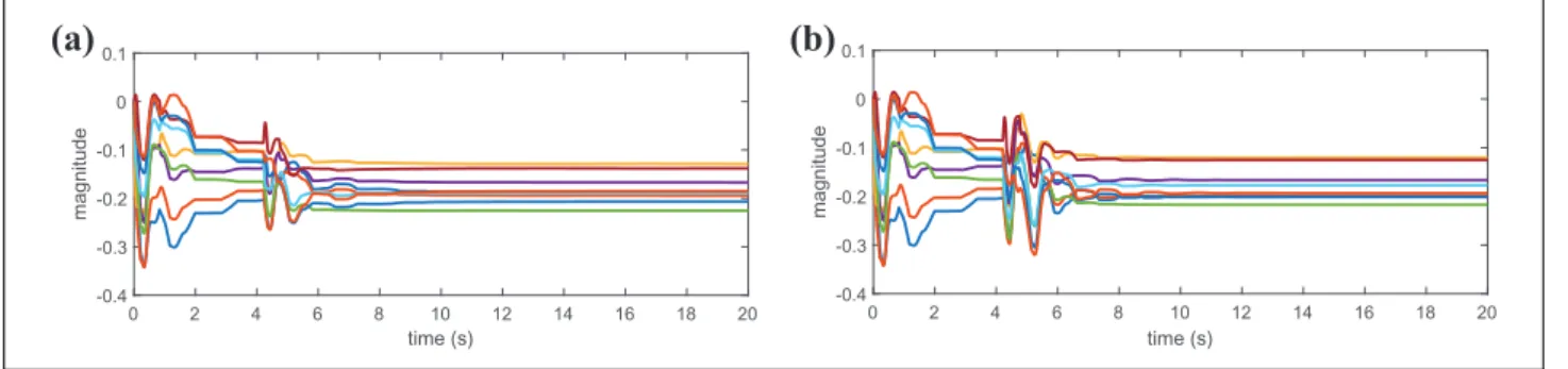
Figure 7.Weights of the RBFNN. (a) Case 1,Ke¼Keproand (b) Case 2,Ke¼Kopte .

Table 2.Feedback gains of differentQE1.

QE1¼0:8 RE¼1:0 QE1¼1:0 RE¼1:0 QE1¼1:2 RE¼1:0 QE1¼1:4 RE¼1:0 QE1¼1:6 RE¼1:0 QE1¼1:8 RE¼1:0 QE1¼2:0 RE¼1:0 Ke1 0.3625 0.5367 0.7205 0.9055 1.0870 1.2620 1.4300 Ke2 0.1090 0.2284 0.3606 0.4968 0.6317 0.7627 0.8884 0 2 4 6 8 10 12 14 16 18 20 -0.4 -0.2 0 0.2 joint position(rad) z1 z2 0 2 4 6 8 10 12 14 16 18 20 time(s) -5 0 5 10 control torque(N/m 2) tau1 tau2 0 2 4 6 8 10 12 14 16 18 20 -0.5 0 0.5 joint position(rad) z₁ z2 0 2 4 6 8 10 12 14 16 18 20 time(s) -10 -5 0 5 10 control torque(N/m 2) tau1 tau2

(a)

(b)

reflect the effectiveness of the proposed ADP controller and admittance control.

Conclusion

The optimal control of robots interacting between unknown environment was studied in this article. An ADP-based controller with admittance adaptation was proposed. The unknown environment was regarded as a linear system and a compliant behaviour was guaranteed by the admittance adaptation control. In addition, NN was introduced into ADP controller to ensure trajectory tracking of the robot with minimal cost. The stability of the robot system was proved and simulation studies demonstrated the effective-ness of the proposed control scheme.

Because of the complexity of the robot system, dynamic uncertainties and input constraints such as saturation and dead zone are very common in robot systems, which will not only affect system performance but also may lead to system instability.24,39,40Therefore, in the frame of ADP, the optimal control problem with dynamic uncertainties and input constraints will be considered in our future work. Declaration of conflicting interests

The author(s) declared no potential conflicts of interest with respect to the research, authorship, and/or publication of this article.

Funding

The author(s) disclosed receipt of the following financial support for the research, authorship, and/or publication of this article: This work was partially supported by Engineering and Physical Sciences Research Council (EPSRC) under grant EP/S001913 and Shenzhen Science and Technology Plan Project [JSGG20180507183020876].

ORCID iD

Chenguang Yang https://orcid.org/0000-0001-5255-5559

References

1. He W, Li Z and Chen CLP. A survey of human-centered intelligent robots: issues and challenges.IEEE/CAA J Autom Sinica2017; 4(4): 602–609.

2. Huang J, Cao Y, Xiong C, et al. An echo state Gaussian process-based nonlinear model predictive control for pneu-matic muscle actuators. IEEE Trans Autom Sci Eng2019; 16(3): 1071–1084.

3. Huang J, Wang Y and Fukuda T. Set-membership-based fault detection and isolation for robotic assembly of electrical con-nectors.IEEE Trans Autom Sci Eng2018; 15(1): 160–171. 4. Chandrasekaran B and Conrad JM. Human–robot

collabora-tion: a survey. In:SoutheastCon 2015, Fort Lauderdale, FL, USA, 9–12 April 2015, pp. 1–8. IEEE.

5. Mason MT. Compliance and force control for computer con-trolled manipulators.IEEE Trans Syst Man Cybern 1981; 11(6): 418–432.

6. Wang C, Li Y, Ge SS, et al. Reference adaptation for robots in physical interactions with unknown environments.IEEE Trans Cybern2017; 47(11): 3504–3515.

7. Huang J, Ri M, Wu D, et al. Interval type-2 fuzzy logic modeling and control of a mobile two-wheeled inverted pen-dulum.IEEE Trans Fuzzy Syst2018; 26(4): 2030–2038. 8. Raibert M and Craig J. Hybrid position/force control of

manipulators.Trans ASME J Dyn Syst Meas Control1981; 103(2): 126–133.

9. Hogan N. Impedance control: an approach to manipulation— Part I: theory; Part II: implementation; Part III: applications. Trans ASME J Dyn Syst Meas Control1981; 107(2): 1–24. 10. Ott C, Mukherjee R and Nakamura Y. A hybrid system

framework for unified impedance and admittance control. J Intell Robot Syst2015; 78(3): 359–375.

11. Braun D, Petit F, Huber F, et al. Optimal torque and stiffness control in compliantly actuated robots. In:2012 IEEERSJ international conference on intelligent robots and systems, Vilamoura, Portugal, 7–12 October, 2012, pp. 2801–2808. 12. Cohen M and Flash T. Learning impedance parameters for

robot control using an associative search network.IEEE Trans Robot Autom1991; 7(3): 382–390.

13. Tsuji T, Ito K and Morasso PG. Neural network learning of robot arm impedance in operational space.IEEE Trans Syst Man Cybern1996; 26(2): 290–298.

14. Love LJ and Book WJ. Force reflecting teleoperation with adaptive impedance control.IEEE Trans Syst Man Cybern 2004; 34(1): 159–165.

15. Uemura M and Kawamura S.Resonance-based motion con-trol method for multi-joint robot through combining stiffness adaptation and iterative learning control. In:2009 IEEE inter-national conference on robotics and automation, Kobe, Japan, 12–17 May 2009, pp. 1543–1548.

16. Gribovskaya E, Kheddar A and Billard A.Motion learning and adaptive impedance for robot control during physical interaction with humans. In:2011 IEEE international confer-ence on robotics and automation, Shanghai, China, 9–13 May 2011, pp. 4326–4332.

17. Stanisic RZ and Fern´andez AV. Adjusting the parameters of the mechanical impedance for velocity, impact and force control.Robotica2012; 30(4): 583–597.

18. Landi CT, Ferraguti F, Sabattini L, et al. Admittance control parameter adaptation for physical human-robot interaction. In:2017 IEEE international conference on robotics and auto-mation (ICRA), Singapore, Singapore, 29 May–3 June 2017, pp. 2911–2916.

19. Yao B, Zhou Z, Wang L, et al. Sensorless and adaptive admit-tance control of industrial robot in physical human–robot interaction.Robot CIM-Int Manuf2018; 51: 158–168. 20. Cervantes I and Alvarez-Ramirez J. On the PID tracking

control of robot manipulators. Syst Control Lett 2001; 42(1): 37–46.

21. Yu W and Rosen J. Neural PID control of robot manipulators with application to an upper limb exoskeleton.IEEE Trans Cybern2013; 43(2): 673–684.

22. Huang J, Zhang M, Ri S, et al. High-order disturbance obser-ver based sliding mode control for mobile wheeled inobser-verted pendulum systems. IEEE Trans Ind Electron2020; 67(3): 2030–2041.

23. Yang C, Teng T, Xu B, et al. Global adaptive tracking control of robot manipulators using neural networks with finite-time learning convergence.Int J Control Autom Syst2017; 15(4): 1916–1924.

24. He W, Dong Y and Sun C. Adaptive neural impedance con-trol of a robotic manipulator with input saturation. IEEE Trans Syst Man Cyber: Syst2016; 46(3): 334–344.

25. Slotine JJE and Li W. On the adaptive control of robot manip-ulators.Int J Robot Res1987; 6(3): 49–59.

26. Fukao T, Nakagawa H and Adachi N. Adaptive tracking con-trol of a nonholonomic mobile robot. IEEE Trans Robot Autom2000; 16(5): 609–615.

27. Huang J, Ri S, Fu T, et al. A disturbance observer based sliding mode control for a class of underactuated robotic system with mismatched uncertainties. IEEE Trans Autom Control2019; 64(6): 2480–2487.

28. Parra-Vega V, Arimoto S, Liu YH, et al. Dynamic sliding PID control for tracking of robot manipulators: theory and experi-ments.IEEE Trans Robot Autom2003; 19(6): 967–976. 29. Zhang S, Dong Y, Ouyang Y, et al. Adaptive neural control

for robotic manipulators with output constraints and uncer-tainties. IEEE Trans Neural Netw Learn 2018; 29(11): 5554–5564.

30. Yang C, Peng G, Li Y, et al. Neural networks enhanced adaptive admittance control of optimized robot–environment interaction.IEEE Trans Cybern2019; 49(7): 2568–2579. 31. Werbos P.Approximate dynamic programming for real-time

control and neural modeling. New York: Van Nostrand Rein-hold, 1992.

32. Wang F, Zhang H and Liu D. Adaptive dynamic program-ming: an introduction.IEEE Comput Intell Mag2009; 4(2): 39–47.

33. Wang D, Liu D and Li H. Policy iteration algorithm for online design of robust control for a class of continuous-time non-linear systems.IEEE Trans Autom Sci Eng 2014; 11(2): 627–632.

34. Liu D, Wang D, Wang FY, et al. Neural-network-based online HJB solution for optimal robust guaranteed cost con-trol of continuous-time uncertain nonlinear systems.IEEE Trans Cybern2014; 44(12): 2834–2847.

35. Wang D, Liu D, Mu C, et al. Neural network learning and robust stabilization of nonlinear systems with dynamic uncer-tainties.IEEE Trans Neural Netw Learn Syst 2018; 29(4): 1342–1351.

36. Jiang Y and Jiang ZP. Computational adaptive optimal con-trol for continuous-time linear systems with completely unknown dynamics.Automatica2012; 48(10): 2699–2704. 37. Siciliano B. A closed-loop inverse kinematic scheme for

on-line joint-based robot control.Robotica1990; 8: 231–243. 38. Corke P. Robotics, vision and control, Vol. 118. Berlin:

Springer, 2017.

39. Sun N, Liang D, Wu Y, et al. Adaptive control for pneumatic artificial muscle systems with parametric uncertainties and unidirectional input constraints. IEEE Trans Ind Inform 2020; 16(2): 969–979.

40. Sun N, Wu Y, Fang Y, et al. Nonlinear antiswing control for crane systems with double-pendulum swing effects and uncertain parameters: design and experiments.IEEE Trans Autom Sci Eng2018; 15(3): 1413–1422.

Appendix 1

This appendix illustrates the stability of the proposed ADP-based controller. For the sake of brevity, the dependency of xwill be omitted, for example, the notationrSðxÞwill be replaced with rS. Besides, define x_ as the optimal time derivative system states corresponding to the optimal con-trol,x_¼ ð f þgÞ ¼f 1 2DrS T_{w. Thus} _ x¼x_þ1 2DrS T_{w~ ð1AÞ}

The Lyapunov candidate is selected as below V ¼ 1 aH ~ wTw~þac 2 x T_{x ð1BÞ}

Combining with equations (7), (38), (41) and (43), its time derivative is _ V ¼ w~T ð1hÞ @E @w^ 0 @ 1 Aþ1 2hacrSDrJs 0 @ 1 A þacrJTsx_ ð1CÞ Case 1. h¼1, namely, ðrJsÞT f 1₂DrSTw^ 0. Then, along with equations (46), (1A) and (1C) is equal to

_ Vj_h¼1¼ ac 1 2w~ T_rSDrJ sþacrJsT x_þ 1 2DrS T_w~ 0 @ 1 A ¼acrJTsx_¼acJ_s<0 ð1DÞ Case 2.h¼0, namely,rJT

sx_<0. In this case, according

to the density property of real numbers, there exists a pos-itive constant lJ such that aclJ k rJsk<acrJTsx_.

Equation (1C) can be rewritten as

_

Vj_h¼0 ¼w~T @E

@w^

þacrJTsx_ ð1EÞ

Equation (44) can also be presented along with equation (42)

@E @w^¼eH @eH @w^ ¼ w~T_rSfþ1 2w~ T_rSDrST_w1 4w~ T_rSDrST_w~e c 0 @ 1 ArSx_ ¼ w~T_rSx__þ1 4kw~k 2 Dþec 0 @ 1 ArS x_þ1 2DrS T_w~ 0 @ 1 A ð1FÞ where D :¼ rSDrST and kxkA¼ ffiffiffiffiffiffiffiffiffiffi xT_Ax p denotes the norm ofxweighting by a compatible matrixA. Substituting equation (1F) into equation (1E) yields

_ V ¼ ðw~TrSx_þ1 4kw~ k 2 DþecÞðw~ T_rSx__þ1 2kw~ k 2 DÞ þacrJsTx_ ¼ 3 4kw~ k 2 Dðw~ T_rSx__{Þ e} cðw~TrSx_þ 1 2kw~ k 2 DÞ 1 8kw~ k 4 Dþðw~TrSx_Þ 2 0 @ 1 AþacrJTsx_ ð1GÞ Assume that l 1 k rS _ xkl1, keckl2, l_d kD kld, ðw~TrSx_Þ2¼kw~TrSx_k2kw~k2k rSx_k2l 2 1 kw~k2 _{and l}4 dkw~k 4 _{kw~ k}4 Dl 4 d kw~k 4_{. Using the} Young’s inequality +ab 1 2r2a 2_þr2 2 b 2 _ð1HÞ we have 3 4kw~ k 2 D w~ T_rSx_ 3 8r2 1 l_d4kw~k4_þ3 8r 2 1l 2 1kw~k 2 ec w~TrSx_ 1 2r2 2 l2 2þ r2 2 2 l 2 1kw~k 2 ec 1 2kw~ k 2 D 1 2r2 3 l2₂þr 2 3 2 l 2 dkw~k 4 1 8kw~ k 4 Dþ w~ T_rSx_ 2 0 @ 1 A 1 8l 4 dkw~k 4_þl2 1kw~k 2 0 @ 1 A acrJTsx_<aclJ k rJsk ð1IÞ

Subsequently, the following inequality holds

_ V <akw~k4_þbkw~k2_þga clJ k rJsk ð1JÞ where a¼1 8l 4 d 3 8r2 1 l_d4þr 2 3 2 l_d2 , b¼3 8r 2 1l 2 1þ r2 2 2 l 2 1l21 andg¼ 1 2r2 2 þ 1 2r2 3

l2₂.r_i are positive numbers required to be chosen appropriately such thata>0

kw~ k ffiffiffiffiffiffiffiffiffiffiffiffiffiffiffiffiffiffiffiffiffiffiffiffiffiffiffiffiffiffiffiffiffiffi bþpffiffiffiffiffiffiffiffiffiffiffiffiffiffiffiffiffiffiffib2þ4ag 2a s ð1KÞ k rJsk ab2þ4a2_g 4a2_l sac ð1LÞ

Finally, if either of the above two inequalities is held,

_

V <0.

To conclude, if equation (1K) or (1L) is satisfied when h¼0, then in both cases, the time derivative of the Lya-punov candidate in equation (1C) is negative which implies the convergence ofw~ and x. This completes the stability analysis.