A COMPARATIVE STUDY OF COLLOCATION METHODS FOR THE NUMERICAL SOLUTION OF DIFFERENTIAL EQUATIONS

COLLOCATION METHODS FOR THE

NUMERICAL SOLUTION OF

DIFFERENTIAL EQUATIONS

By

MARGARET MODUPE KAJOTONI

academic requirements for the degree of

Master of Science in the

School of Mathematical Sciences

University of KwaZulu-Natal

Durban

Abstract

The collocation method for solving ordinary differential equations is examined. A detailed comparison with other weighted residual methods is made. The orthogonal collocation method is compared to the collocation method and the advantage of the former is illustrated. The sensitivity of the orthogonal collocation method to different parameters is studied. Orthogonal collocation on finite elements is used to solve an ordinary differential equation and its superiority over the orthogonal collocation method is shown. The orthogonal collocation on finite elements is also used to solve a partial differential equation from chemical kinetics. The results agree remarkably with those from the literature.

Mr and Mrs R.O. Kajotoni

Acknowledgments

I will remain grateful to the founder of AIMS, professor Neil Turok and its director, professor Fritz Hahne for giving me such an exceptional opportunity to realize my dreams. My gratitude also goes to the entire AIMS family. I acknowledge the University of KwaZulu-Natal research office and professor Jacek Banasiak for also providing funding for this work.

I feel indebted to my supervisor, Dr P. Singh for all his reliable guidance and commitments throughout the course of my study. His approach to problem solving will definitely help me in future. I also appreciate the enormous contribution of my co-supervisor, Dr N. Parumasur.

Many thanks to my parents, Mr and Mrs R.O. Kajotoni for their expression of love. I also acknowledge the contributions of my brothers Kayode and Tunde and my sister Mrs Ojerinde and her family. To the Eniolorunda’s and Kajotoni’s home and abroad, I say thank you all.

My irrevocable gratitude goes to my beloved fiance Raphael Olushola Folorunsho for his love, patience and tactfulness throughout my stay in South Africa. Many thanks to the Folorunsho’s for all their love and concern.

My appreciation also goes to Faye, Salvie, Mrs Petro, Mrs Henning, Dr P. Pillay, Dr Moopanar, prof Baboolal Dharmanand, Dr Kutu and family, Annemarie, Soren, Simon, Lucie, Mary, Emmanuel, Alfred, Elmah, Rudo, Ivy, Iyabo, Lola and all my colleagues in the School of Mathematical Sciences for all their love and hospitality.

Christian Church Durban and The Redeemed Christian Church of God(RCCG) Durban for being part of my life and for all their kind gestures which has led to the successful completion of my study.

My utmost gratitude goes to my Lord and my personal saviour, Jesus Christ for enabling me accomplish this dissertation.

Preface

I Margaret Modupe Kajotoni affirm that the work in this thesis was carried out in the School of Mathematical Sciences, University of KwaZulu-Natal, Durban, during the period of August2007to October2008. It was completed by the author under the supervision of Dr P. Singh and co-supervised by Dr N. Parumasur.

The research contained in this thesis has not been submitted to any University nor has it been published previously. Where use was made of the work of others it has been duly acknowledged in the text.

MM Kajotoni October 2008

Declaration-Plagiarism

I Margaret Modupe Kajotoni declare that

1. The research reported in this thesis, except where otherwise indicated, is my original research.

2. This thesis has not been submitted for any degree or examination at any other university.

3. This thesis does not contain other persons’ data, pictures, graphs or other information, unless specifically acknowledged as being sourced from other persons.

4. This thesis does not contain other persons’ writing, unless specifically ac-knowledged as being sourced from other researchers. Where other written sources have been quoted, then:

a. Their words have been re-written but the general information attributed to them has been referenced.

b. Where their exact words have been used, then their writing has been placed in italics and inside quotation marks, and referenced.

5. This thesis does not contain text, graphs or tables copied and pasted from the Internet, unless specifically acknowledged, and the source being detailed in the thesis and in the Reference sections.

Signed: Date:

Notation

L Linear differential operator

R Residual

φi Basis function

w(x) Weight function

K Condition number

X Domain of interest

C(X) Continuous function over the domain X y Exact solution to differential equations

ya Approximate solution to weighted residual methods

ea Error from the approximate solution ya

yc Approximate solution by the collocation method

ys Approximate solution by the sub-domain method

yl Approximate solution by the least square method

ym Approximate solution by the moment method

yg Approximate solution by the Galerkin method

k · k2 Euclidean norm inRn

h , _i Inner product onC(X)

N Order of polynomial

TN Chebyshev Polynomial of the first kind of order N

UN Chebyshev Polynomial of the second kind of orderN

PN Legendre Polynomial of order N

lk Lagrange polynomial function

ψ(x) Nodal polynomials

Ne Number of finite elements

hi Length of the ith element

yi Approximate solutions using equally spaced finite elements

ei Error from the approximate solution yi

¯

yi Approximate solutions using unequally spaced finite elements

¯

ei Error from the approximate solution y¯i

ye Exit solution

P Peclet number

List of Tables

1.1 Numerical comparison of the different approximations in Example 1.3.1. . . 13

1.2 Approximate solutions for Example 1.3.2. . . 14

1.3 Numerical comparison of the different approximations in Example 1.3.2. . . 16

1.4 Numerical comparison of the different approximations in Example 1.3.3. . . 22

1.5 Numerical comparison of y, yc and y¯c for Example 1.3.3. . . 25

2.1 Numerical comparison for one point collocation for Example 2.5.1 with α= 1and order N = 2. . . 39

2.2 Numerical comparison for one point collocation for Example 2.5.1 with α= 10 and order N = 2. . . 40

2.3 Numerical comparison of the errors for Example 2.5.1 for different ordersN, with collocation points chosen as the shifted roots ofTN₋1,

UN−1 and PN−1 respectively. . . 46

2.4 Numerical comparison for Example 2.5.2 for order N = 3, with collocation points chosen as roots of T₂. . . 50

ferent orders, with collocation points chosen as the roots of TN−1,

UN₋1 and PN₋1 respectively. . . 56

3.1 Numerical comparison of y, y2 and ¯y2 at different values of x. . . 65

3.2 Numerical comparison of y₃ and ¯y₃. . . 69 3.3 Total error as a function of the number of elements(i) for equal and

unequal element spacing. . . 71

List of Figures

1.1 Comparison ofy and y_a for Example 1.3.1. . . 11

1.2 Errors ea=y −ya for Example 1.3.1. . . 11

1.3 Comparison ofy and ya for Example 1.3.2. . . 15

1.4 Errors ea=y −ya for Example 1.3.2. . . 17

1.5 Comparison ofy and y_a for Example 1.3.3. . . 21

1.6 Errors ea=y −ya for Example 1.3.3. . . 21

1.7 Comparison ofy, yc and y¯c for Example1.3.3. . . 24

1.8 Errors ec =y −yc and e¯c =y −y¯c for Example1.3.3. . . 24

2.1 Comparison of y and y_a for Example 2.5.1 with α = 1 and order N = 2. . . 37

2.2 Error between y and ya for Example 2.5.1 with α = 1 and order N = 2. . . 37

2.3 Comparison of y and y_a for Example 2.5.1 with α = 10 and order N = 2. . . 38

2.4 Error between y and ya for Example 2.5.1 with α = 10 and order N = 2. . . 38

with collocation points chosen as the shifted roots ofTN−1. . . 42

2.6 Errors for Example 2.5.1 for orders N = 3, 4, 5, with collocation points chosen as the shifted roots ofTN−1. . . 43

2.7 Error for order N = 16 for Example 2.5.1, with collocation points chosen as the shifted roots ofT15. . . 43

2.8 Comparison of y and ya for Example 2.5.1 for orders N = 3, 4, 5,

with collocation points chosen as the shifted roots ofUN−1. . . 44

2.9 Errors for Example 2.5.1 for orders N = 3, 4, 5, with collocation points chosen as the shifted roots ofUN−1. . . 45

2.10 Comparison of y and ya for Example 2.5.1 for orders N = 3, 4, 5,

with collocation points chosen as the shifted roots ofPN−1. . . 45

2.11 Errors for Example 2.5.1 for orders N = 3, 4, 5, with collocation points chosen as the shifted roots ofPN−1. . . 46

2.12 Comparison of y and ya for Example 2.5.2 for order N = 3, with

collocation points chosen as roots of T2. . . 49

2.13 Error for Example 2.5.2 for order N = 3, with collocation points chosen as rootsT2. . . 51

2.14 Comparison ofy andy_a for Example 2.5.2for orders N = 4, 6, 8, 10, with collocation points chosen as the roots ofTN−1. . . 53

2.15 Errors for Example 2.5.2 for orders N = 4, 6, 8, 10, with collocation points chosen as the roots of TN−1. . . 53

2.16 Error for order N = 20 for Example 2.5.2, with collocation points chosen as the roots ofT19. . . 54

with collocation points chosen as the roots ofUN−1. . . 54

2.18 Errors for Example 2.5.2 for orders N = 4, 6, 8, 10, with collocation points chosen as the roots of UN−1. . . 55

2.19 Comparison ofy andya for Example 2.5.2for orders N = 4, 6, 8, 10, with collocation points chosen as the roots ofPN−1. . . 55

2.20 Errors for Example 2.5.2 for OrdersN = 4, 6, 8, 10, with collocation points chosen as the roots of PN−1. . . 56

3.1 Arrangement of sub-domains in the OCFE method. . . 59

3.2 Arrangement of the collocation points in the ith element [xi,xi+1]. . . 60

3.3 Comparison ofy, y₂ and y¯₂. . . 64 3.4 Errors e2 =y −y2 and ¯e2 =y −¯y2. . . 64 3.5 Comparison ofy, y₃ and y¯₃. . . 68 3.6 Errors e3 =y −y3 and ¯e3 =y −¯y3. . . 68 3.7 Comparison ofy, y₆ and y¯₆. . . 70 3.8 Errors e6 =y −y6 and ¯e6 =y −¯y6. . . 70 3.9 Errors ei =y −yi. . . 71

3.10 Global and local numbering of coefficients for the OCFE method. . 72

4.1 Error ye₁₋y₇ at x = 1 forP = 0.8. . . 78

4.2 Comparison ofye2 and y3 atx = 1for P = 20. . . 79

4.3 Error ye₂₋y₃ at x = 1 forP = 20. . . 79

4.4 Errors ei =ye2 −yi at x = 1 forP = 20 . . . 80

4.6 Error e43 =ye43−y43 atx = 1 for P = 40 . . . 81

4.7 Comparison ofy with yi att = 0.001 forP = 40. . . 82

4.8 Errors ei =y −yi att = 0.001for P = 40 . . . 82

4.9 Comparison ofy with yi att = 1for P = 40. . . 83

4.10 Errors ei =y −yi att = 1for P = 40. . . 83

4.11 Comparison of y with yi att = 2for P = 40 . . . 84

4.12 Errors ei =y −yi att = 2for P = 40. . . 84

4.13 Comparison of y and y₅₀ att = 0.001for P = 40. . . 85

4.14 Error y ₋y50 att = 0.001 forP = 40. . . 85

4.15 Error y ₋y₅₀ att = 1 for P = 40. . . 86

4.16 Error y ₋y50 att = 2 for P = 40. . . 86

4.17 Almost perfect mixing for y₇ at x = 1 forP = 1.0_×10−5_{. . . . 89}

4.18 Almost perfect displacement at x = 0.4 for y100 for P = 1000. . . 89

4.19 Solution for y₁₀₀ and ye₁ from equation (4.22) for P = 0.8. . . 90

Contents

Introduction 1

1 Method of Weighted Residuals 2

1.1 Introduction . . . 2

1.2 Variation on Theme of Weighted Residuals . . . 4

1.2.1 Collocation Method . . . 4

1.2.2 Sub-domain Method . . . 5

1.2.3 Least Squares Method . . . 6

1.2.4 Moment Method . . . 6

1.2.5 Galerkin Method . . . 7

1.3 Numerical Examples . . . 7

1.3.1 Two Terms Trial Solution for a Slow Reaction Rate . . . 8

1.3.2 Two Terms Trial Solution for a Fast Reaction Rate . . . 14

1.3.3 Three Terms Trial Solution for a Fast Reaction Rate . . . . 17

1.3.4 Different Choice of Collocation Points . . . 23

2 Orthogonal Collocation Method 26

2.2 Orthogonal Polynomials . . . 27

2.2.1 Useful Properties of Orthogonal Polynomials . . . 27

2.2.2 Chebyshev Polynomials of the First Kind TN(x) . . . 28

2.2.3 Chebyshev Polynomials of the Second Kind UN(x) . . . 29

2.2.4 Legendre Polynomials PN(x) . . . 29

2.3 Lagrange Interpolation . . . 30

2.3.1 Chebyshev Interpolation Nodes . . . 33

2.4 Relationship Between Galerkin and Collocation Method . . . 33

2.5 Numerical Examples . . . 35

2.5.1 One Point Collocation for Example 2.5.1 . . . 35

2.5.2 Generalization of Example 2.5.1 . . . 41

2.5.3 Two Points Collocation for Example 2.5.2 . . . 47

2.5.4 Generalization of Example 2.5.2 . . . 49

3 Application of Orthogonal Collocation on Finite Elements (OCFE) to Solving ODE’s 57 3.1 Introduction . . . 57

3.2 Methodology . . . 58

3.2.1 Distribution of Elements . . . 60

3.3 Numerical Example . . . 60

3.3.1 Two Finite Elements for Example 3.3.1 . . . 61

4 Application of Orthogonal Collocation on Finite Elements (OCFE) to Solving PDE’s 73 4.1 Introduction . . . 73 4.2 Numerical Example . . . 74 4.2.1 Exit Solution . . . 74 4.2.2 General Solution . . . 81 4.2.3 Limiting Cases . . . 87 5 Conclusion 91 5.1 Conclusion . . . 91 References 96 Appendices 104

A Programme for Example 2.5.1 104

B Programme for Example 2.5.2 109

C Programme for Example 3.3.1 114

D Programme for Example 4.2.1 119

E First 17 Roots of (4.17), P=0.8. 125

Introduction

Differential equations are used for mathematical modeling in science and engineer-ing. However, it is apparent that there may be no known analytic solution to such differential equations and even when it does exist it might be very difficult to ob-tain. In such cases, the numerical approximations are used. Of special interest are numerical techniques that reduce excessive demand for computational time and at the same time giving a close approximation to the exact solution.

In this thesis, we present a simple but effective numerical technique called the orthogonal collocation method for solving differential equations.

Chapter1gives an overview of the five different methods of weighted residuals. We introduce the orthogonal collocation method in chapter2. Chapter 3explains the features of the orthogonal collocation method on finite elements and it is then used to solve an ODE. Chapter4gives a practical example of the orthogonal collocation on finite elements applied to a PDE problem in chemical engineering. Each chapter gives the details of the numerical procedures used.

Chapter 1

Method of Weighted Residuals

1.1

Introduction

The method of weighted residuals was used to find approximate solutions to dif-ferential equations before the finite element method came into existence [21]. The method was introduced by Crandall [16] in 1956 . Other scientists like Finlayson and Scriven (1966) [23], Vichnevetsky (1969) [71] and Finlayson (1972) [22] have also used this method. The method is used to solve boundary value problems arising from fluid flow, structural mechanics and heat transfer. It is well known because of the interactive nature of the first step. The user provides an initial guess for the solution which is then forced to satisfy the governing differential equations and its boundary conditions. The guessed solution is chosen to satisfy the bound-ary conditions, however it does not necessarily satisfy the differential equations [28, 59].

The method of weighted residuals requires two types of functions namely the trial functions and the weight functions. The former is used to construct the trial solution while the latter is used as a criterion to minimize the residual [21].

Consider a linear differential equation

L y(x) =f(x), (1.1)

together withk boundary conditions. HereL is a bounded linear differential oper-ator and f(x)_∈C(X), where X denotes the domain. The unknown solution y(x) is approximated by a function ya(x) and we write

y(x)_≈ya(x) = N

X

i=1

ciφi(x), (1.2)

where the set _{φi(x)|i = 1, 2, ...,N} constitutes a basis for a finite dimensional

subspace ofC(X)and theci’s are constant coefficients. When substituted into the

differential equation (1.1) we obtain

L ya(x) = fa(x), (1.3)

where in general

fa(x)6=f(x). (1.4)

Subtracting equation (1.1) from equation (1.3) yields the residual equation

R(x) = L(ya(x)−y(x)) =L ya(x)−L y(x) =L ya(x)−f(x)6= 0. (1.5)

From equation (1.5), it is easy to show that

kya(x)−y(x)k=kL−1R(x)k ≤ k

L_kkL−1_k

kL_k kR(x)k= K

kL_kkR(x)k, (1.6)

where K is the condition number of L and _{k · k} denotes compatible operator and function norms on C(X). Hence for a well conditioned problem, the closer the residual is to zero, the better is the approximate solution. The unknown coefficients

ci’s are chosen to force the residual to zero in some average sense over the domain

X by requiring that Z

X

R(x)wi(x) dx = 0, i = 1, 2, ...,N −k, (1.7)

where the weight functions wi(x) are specified and we require N −k of them to

yield N ₋k equations which together withk boundary conditions are sufficient to determine the unknowns c_i.

1.2

Variation on Theme of Weighted Residuals

There are five widely used variations of the method of weighted residuals for engi-neering and science applications, namely

1. The collocation method,

2. The sub-domain method,

3. The least squares method,

4. The moment method,

5. The Galerkin method.

The distinguishing factor between these methods is the choice of the weight func-tions used in minimizing the residual. We shall briefly discuss the different features of each method.

1.2.1

Collocation Method

In this method, the weight functions are taken from the family of the Dirac delta (δ) functions in the domain X, that is wi(x) = δ(x−xi). The Dirac delta function

is defined by [47] δ(x ₋xi) =      1 x =xi, 0 otherwise (1.8)

and has the property that Z

X

f(x)δ(x₋xi)dx =f(xi). (1.9)

Hence the integration of the weighted residual (1.7) results in forcing the residual to zero at specific points in the domain. That is, with this choice of the weight function, equation (1.7) reduces to

Z

X

As the number of collocation pointsxi increases, we satisfy the differential equation

at more points and hence force the approximate solution to approach the exact solution. The ease of performing integrals with the Dirac delta function is an added advantage of the collocation method.

The collocation method was first used by Frazer et al [24] in 1937 . Thereafter Bickley [7] used it in 1941 along with the least squares method and the Galerkin method to solve unsteady heat condition problems. In 1962, Jain introduced an extremal-point collocation by sampling the residual at the zerosxi of the Chebyshev

polynomials and requiring that

R(xi+1)−(−1)iR(x1) = 0, i = 1, 2, ...,N−k. (1.11)

He chose the zeros of the Chebyshev polynomials because they are known to min-imize the maximum error [30]. Jain combined this method with the Newton’s method to solve a viscous fluid problem.

In1963, Schetz applied the low-order collocation method to a number of boundary-layer problems [63]. In 1975, Panton and Sallee applied a collocation method to problems of unsteady heat conduction and boundary layer flows [52]. They usedB -splines as trial functions and compared their results with results obtained from the finite-difference method. The results were more accurate than those obtained from the finite-difference method. Viviand and Ghazzi in 1974 applied a collocation method to the problem of computing the viscid flow about an inclined three-dimensional wing [74].

The collocation method has been used over a wide range of problems in recent times [15, 32, 68, 70].

1.2.2

Sub-domain Method

Here the weight function is always w(x) _≡ 1. The domain is split into N ₋k

ci, hence Z X R(x)wi(x)dx = N−k X i=1 Z Xi R(x)dx . (1.12)

This method forces the residual to be zero over the various sub-domains, that is Z

Xi

R(x)dx = 0. (1.13)

This method originated from the work of Biezeno and Koch in 1923 [8]. Pallone [51] and Bartlett [5] used it to solve Laminar boundary layers and Murphy has used it to solve incompressible Navier-Stokes equations [46] .

1.2.3

Least Squares Method

In this method, we minimize the Euclidean norm of the residual, namely

S =_kR(x)_k2₂ = Z

X

R2(x)dx. (1.14)

To obtain the minimum of this scalar function, the derivatives of S with respect to the unknown parameters ci must be zero. This yields,

Z

X

R(x)∂R(x)

∂ci

dx = 0. (1.15)

Comparing equation (1.7) and equation (1.15), the weight functions for the least squares method are identified as the derivatives of the residual with respect to the unknown constants:

wi(x) =

∂R(x)

∂ci

. (1.16)

The least squares method is the oldest of all the methods of weighted residuals [25]. Crandall stated in his work in 1956 that “the least square method was discovered by Gauss in 1775” [16]. In 1937, Frazer et al [24] also used this method.

1.2.4

Moment Method

In this method, the weight functions are chosen from the family of polynomials. That is

In 1948, Yamada applied this method to a nonlinear diffusion problem [77]. His formulation is described in Ames [2].

1.2.5

Galerkin Method

This method is a modification of the least squares method. The weight functions are chosen as the derivative of the approximating function with respect toci, that

is

wi(x) =

∂ya(x)

∂ci

. (1.18)

From equation (1.2), it is easily seen that wi(x) is identical to the basis function

φi(x). Hence the unknownsci are determined so that the residual R(x)is

perpen-dicular to the subspace spanned by _{φi p(x)|p = 1, 2, ...,N −k} where

{ip|p= 1, 2, ...,N −k} ⊆ {1, 2, ...,N}.

This method was first introduced by Galerkin in1915[26]. Duncan used it to study the dynamics of aeronautical structures [19, 18]. It was later used by Bickley to solve unsteady heat conduction problems [7].

1.3

Numerical Examples

We illustrate the five variations of the method of weighted residuals with some examples.

Example 1.3.1 Consider the differential equation defined on[0, 1]with its

bound-ary conditions which represents a diffusion-reaction equation in chemistry given by

d2_y dx2 + dy dx −α 2_{y = 0,} y′(0) = 0, y(1) = 1, (1.19)

where α is a constant parameter that denotes the reaction rate which is termed slow for small values of α and fast for larger α’s. The solution y(x) describes the concentration of a chemical substance at distance x.

The exact solution to this equation is given by

y(x) = e (1 2− x 2) (2βcosh (β_x) + sinh (β_x)) 2βcosh (β) + sinh (β) , (1.20) whereβ = √4α2₊₁

2 . We find an approximate solution to equation (1.19), with α= 1

using the five different methods of weighted residuals.

1.3.1

Two Terms Trial Solution for a Slow Reaction Rate

Let us pick the trial solution from a subspace of dimension two ofC[0, 1]as

ya(x) =c1+c2(1−x2). (1.21)

Hereφ1(x) = 1andφ2(x) = (1−x2)are the basis functions. The requirement that

y_a(x)satisfies the boundary conditiony(1) = 1implies thatc₁ = 1. It is noted that the boundary conditiony′(0) = 0is automatically satisfied byya(x)because of the

clever choice of the basis function φ2(x). We therefore need one more condition to

evaluate c₂.

Substituting the trial solution in equation (1.21) into the differential equation (1.19) gives the residual (since f(x) = 0):

R(x) =₋2c₂₋2c₂x ₋(1 +c₂(1₋x2)). (1.22) Substituting the residual in equation (1.22)into equation (1.7) gives

hR(x),w₁(x)_i= Z 1

0

−2c₂₋2c₂x₋(1 +c₂(1₋x2))w₁(x)dx = 0, (1.23) where _h , _i denotes the inner product on C[0, 1]. We evaluate c2 by choosing

1. The Collocation Method

The test function is w1(x) = δ(x −x1), where x1 is the unknown

colloca-tion point which must be chosen from the domain [0, 1]. So equation (1.23) becomes hR(x),w₁(x)_i= Z 1 0 −2c₂₋2c₂x₋(1 +c₂(1₋x2))δ(x₋x₁)dx. (1.24) Applying the property of the Dirac delta function (see equation(1.10)) gives

−2c2−2c2x1−(1 +c2(1−x12)) = 0, (1.25)

and simplifying yields c₂ = _(2+2x−1

1+(1−x12))

. Choosing x₁ = 0.5, we obtain

c2 =−4/5 and the trial solution by the collocation method is,

yc(x) = 1−4(1−x2)/5. (1.26)

2. Sub-domain Method

Since we have only one unknown, we only need one sub-domain which is the whole domain [0, 1]. Hence the weight function is w₁(x) = 1, for 0 _≤x _≤ 1 and equation (1.23) becomes

hR(x),w1(x)i= Z 1 0 −2c2−2c2x −(1 +c2(1−x2)) dx = 0. (1.27)

Integrating with respect to x and evaluating givesc₂ =₋3/11. Hence the trial solution by the sub-domain method is

ys(x) = 1−3(1−x2)/11. (1.28)

3. The Least Squares Method

The weight function is w1 = _∂∂_cR₂ and equation (1.23) becomes

Z 1 0 R∂R ∂c₂dx = 1 2 ∂ ∂c₂ Z 1 0 −2c2−2c2x −(1 +c2(1−x2)) 2 dx = 0. (1.29)

Integrating with respect to x and then differentiating with respect to c₂ we obtain c2 =−55/203. Hence the trial solution by the least squares method

is

4. The Moment Method

The weight function isw1 =x0 = 1which is similar to that of the sub-domain

method. Since only two terms are retained with one unknown, the solution will be the same as that of the sub-domain method, hence

ym(x) = 1−3(1−x2)/11. (1.31)

5. Galerkin Method

The weight function is the same as that of the trial function, so we choose

w₁(x) = (1₋x2). Thus equation (1.23) becomes hR(x),w1(x)i= Z 1 0 −2c2−2c2x −(1 +c2(1−x2)) (1₋x2)dx. (1.32) Integrating and evaluating gives c2 = −20/71. Hence the trial solution by

the Galerkin method is

yg(x) = 1−20(1−x2)/71. (1.33)

The plots of the solutions and the errors for the above five methods are given in Figures 1.1 and 1.2 respectively.

0 0.2 0.4 0.6 0.8 1 0.7 0.75 0.8 0.85 0.9 0.95 1 Distance, x Solution y g y y c y_s y_l

Figure 1.1: Comparison of y and ya for Example 1.3.1.

0 0.2 0.4 0.6 0.8 1 −0.02 −0.015 −0.01 −0.005 0 0.005 0.01 Distance, x Error e g e c e l e s

We will sample the exact solution y(x) and the approximate solutions ya(x) at a

discrete set of twenty one equally spaced pointsxi, i = 1, 2, ..., 21and denote these

vectors by y¯(x)and y¯a(x). We define the total error by

total error =_k¯y(x)₋y¯a(x)k2, (1.34)

where _{k · k}2 denotes the Euclidean norm in R21.

Table 1.1 gives the approximations and the total error for Example 1.3.1 for dif-ferent values of x.

The results of the numerical solutions for different values ofx agree closely with the analytic solutions (see Figure 1.1). Moreover, all the methods show small errors (see Figure 1.2) and the solution values agree closely with the exact solution (see Table 1.1) even though only two terms were retained in the trial solution. This is because of the slow reaction rate α= 1. Hence the concentration profile of the chemical substance is shallow and can easily be described by only two terms. From Table 1.1, we see that the Galerkin method has a slightly lower total error and hence gives the best approximation to this particular problem. If we allow a higher reaction rate, the concentration profile becomes steep and the trial solution with two terms is unable to track the solution. Let us illustrate this by picking α= 10 in equation (1.19).

x y yc ys yl yg 0 0.7157 0.7333 0.7273 0.7291 0.7183 0.0500 0.7165 0.7340 0.7280 0.7297 0.7190 0.1000 0.7191 0.7360 0.7300 0.7318 0.7211 0.1500 0.7233 0.7393 0.7334 0.7352 0.7246 0.2000 0.7291 0.7440 0.7382 0.7399 0.7296 0.2500 0.7364 0.7500 0.7443 0.7460 0.7359 0.3000 0.7451 0.7573 0.7518 0.7534 0.7437 0.3500 0.7552 0.7660 0.7607 0.7623 0.7528 0.4000 0.7666 0.7760 0.7709 0.7724 0.7634 0.4500 0.7794 0.7873 0.7825 0.7839 0.7753 0.5000 0.7935 0.8000 0.7955 0.7968 0.7887 0.5500 0.8087 0.8140 0.8098 0.8110 0.8035 0.6000 0.8253 0.8293 0.8255 0.8266 0.8197 0.6500 0.8430 0.8460 0.8425 0.8435 0.8373 0.7000 0.8619 0.8640 0.8609 0.8618 0.8563 0.7500 0.8820 0.8833 0.8807 0.8815 0.8768 0.8000 0.9033 0.9040 0.9018 0.9025 0.8986 0.8500 0.9257 0.9260 0.9243 0.9248 0.9218 0.9000 0.9493 0.9493 0.9482 0.9485 0.9465 0.9500 0.9741 0.9740 0.9734 0.9736 0.9725 1.0000 1.0000 1.0000 1.0000 1.0000 1.0000 Total error _⇒ 0.0455 0.0274 0.0325 0.0165

1.3.2

Two Terms Trial Solution for a Fast Reaction Rate

We now solve equation (1.19) with a fast reaction rate relative to diffusion.

Example 1.3.2 Using only two terms as in Example 1.3.1 and picking α= 10 in

Equation (1.19), our residual becomes

R(x) =₋2c₂₋2c₂x₋100 1 +c₂(1₋x2). (1.35) We will again apply the five different weighted residuals methods as in Example 1.3.1. The summary of the approximate solutions using the five different methods is given in Table 1.2. Hence forth we will approximate the coefficients to four decimal places.

Method Approximate Solution

Collocation yc(x) = 1−1.2821(1−x2)

Sub-domain ys(x) = 1−1.4354(1−x2)

Least squares yl(x) = 1−1.2202(1−x2)

Moment ym(x) = 1−1.4354(1−x2)

Galerkin yg(x) = 1−1.2085(1−x2)

Table 1.2: Approximate solutions for Example 1.3.2.

The plots of the solutions and their errors are shown in Figures1.3and 1.4 respec-tively. A table of values resulting from the different approximations is shown in Table 1.3.

We notice from Figure1.3that the approximate solutions deviate sharply from the exact solution hence the error between the approximate and the exact solution is large (See Figure 1.4). This is due to the sharp concentration profile. We notice from Table 1.3 that even the Galerkin method which on the average is the best approximation is still not a very good approximation to the exact solution. We

can reduce the error by increasing the dimension of the approximation space. In general, the more terms used in the trial solution, the better the accuracy but the computation becomes expensive.

0 0.2 0.4 0.6 0.8 1 −0.5 0 0.5 1 Distance, x Solution y l y_c y s y g y

x y yc ys yl yg 0 0.0001 ₋0.2821 ₋0.4354 ₋0.2202 ₋0.2085 0.0500 0.0002 ₋0.2789 ₋0.4318 ₋0.2171 ₋0.2055 0.1000 0.0002 ₋0.2693 ₋0.4210 ₋0.2080 ₋0.1964 0.1500 0.0003 ₋0.2533 ₋0.4031 ₋0.1927 ₋0.1813 0.2000 0.0005 ₋0.2308 ₋0.3780 ₋0.1714 ₋0.1602 0.2500 0.0008 ₋0.2020 ₋0.3457 ₋0.1439 ₋0.1330 0.3000 0.0013 ₋0.1667 ₋0.3062 ₋0.1104 ₋0.0997 0.3500 0.0021 ₋0.1250 ₋0.2596 ₋0.0707 ₋0.0605 0.4000 0.0033 ₋0.0770 ₋0.2057 ₋0.0250 ₋0.0151 0.4500 0.0053 ₋0.0225 ₋0.1447 0.0269 0.0362 0.5000 0.0086 0.0384 ₋0.0766 0.0849 0.0936 0.5500 0.0138 0.1057 ₋0.0012 0.1489 0.1571 0.6000 0.0223 0.1795 0.0813 0.2191 0.2266 0.6500 0.0358 0.2596 0.1711 0.2953 0.3021 0.7000 0.0576 0.3461 0.2679 0.3777 0.3837 0.7500 0.0927 0.4391 0.3720 0.4662 0.4713 0.8000 0.1492 0.5384 0.4833 0.5607 0.5649 0.8500 0.2401 0.6442 0.6017 0.6614 0.6646 0.9000 0.3863 0.7564 0.7273 0.7682 0.7704 0.9500 0.6215 0.8750 0.8600 0.8810 0.8822 1.0000 1.0000 1.0000 1.0000 1.0000 1.0000 Total error _⇒ 1.1154 1.3327 1.0854 1.0841

0 0.2 0.4 0.6 0.8 1 −0.5 −0.4 −0.3 −0.2 −0.1 0 0.1 0.2 0.3 0.4 0.5 Distance, x Error e l e c e s e g

Figure 1.4: Errorsea =y −ya for Example1.3.2.

1.3.3

Three Terms Trial Solution for a Fast Reaction Rate

We seek to improve the accuracy of the results obtained in Example1.3.2by using a subspace of dimension three.

Example 1.3.3 In order to improve the accuracy of the solution for a fast reaction

rateα= 10, we retain three terms in the trial solution. Hence the new trial solution is

ya =c1+c2(1−x2) +c3x2(1−x2), (1.36)

where the basis functions are _{1, 1₋x2_,x2_(1−x2_{)} and c}

1 = 1 because of the

boundary conditiony(1) = 1in equation(1.19). The boundary conditiony′(0) = 0 is automatically satisfied by ya(x).

The residual becomes

R(x) =₋2c2+ 2c3 −12c3x2−2c2x + 2c3x −4c3x3

−100(1 +c₂(1₋x2) +c₃x2(1₋x2)).

1. The Collocation Method

Since we have two unknowns, we will need two weight functions given by

w₁(x) =δ(x ₋x₁) and w₂(x) =δ(x ₋x₂) , where x₁ and x₂ are the unknown collocation points which we choose as x1 = 1/3 and x2 = 2/3. Next we

evaluate the following two inner products

hR(x),w1(x)i= Z 1 0 [R(x)δ(x ₋x1)]dx = 0 (1.38) and hR(x),w2(x)i= Z 1 0 [R(x)δ(x₋x2)]dx = 0, (1.39)

by applying the property of the Dirac delta function (equation (1.10)), and evaluating at the collocation points x₁ = 1/3 and x₂ = 2/3to obtain

R(x1) = 0 (1.40)

and

R(x2) = 0. (1.41)

Simplifying equations (1.40) and (1.41) yields the linear system

−91.5577c₂₋8.6894c₃ = 100

−58.8845c₂₋27.8778c₃ = 100, (1.42)

which we solve simultaneously to yield c2 =−0.9403 and c3 =−1.6010. So

the trial solution by the collocation method is

yc(x) = 1−0.9403(1−x2)−1.6010x2(1−x2). (1.43)

2. Sub-domain Method

Since we have two unknowns, we will split the interval [0, 1] into two sub-domains: [0, 0.5] and [0.5, 1]. The weight functions are w1(x) = w2(x) = 1.

So we will need to evaluate the following two inner products

hR(x),w1(x)i=

Z 0.5 0

and

hR(x),w2(x)i=

Z 1 0.5

R(x)dx = 0. (1.45)

These give the linear system

−47.0833c2−2.8542c3 = 50

−22.5833c2−12.4792c3 = 50, (1.46)

which we solve simultaneously to yield c₂ = ₋0.9200 and c₃ = ₋2.3418. Hence the trial solution by the sub-domain method is

ys(x) = 1−0.9200(1−x2)−2.3418x2(1−x2). (1.47)

3. The Least Squares Method

The weight functions are w₁ = ∂R

∂c2 and w2 =

∂R

∂c3. So we will need to evaluate

the following inner products

hR(x),w₁(x)_i= Z 1 0 R∂R ∂c2 dx = 1 2 ∂ ∂c2 Z 1 0 R2(x)dx = 0 (1.48) and hR(x),w₂(x)_i= Z 1 0 R∂R ∂c₃dx = 1 2 ∂ ∂c₃ Z 1 0 R2(x)dx = 0. (1.49) Integrating equations (1.48) and (1.49) with respect to x and then differen-tiating with respect to c₂ and c₃ respectively gives the linear system

11418.70c2+ 1647.01c3 = 13933.30

1647.01c₂+ 717.10c₃ = 3066.67, (1.50)

which we solve simultaneously to obtain c₂ = ₋0.9029 and c₃ = ₋2.2000. Hence the trial solution by the least squares method is

yl(x) = 1−0.9029(1−x2)−2.2000x2(1−x2). (1.51)

4. The Moment Method

Here the weight functions are w₁ = 1 and w₂(x) = x. So we will need to evaluate the integrals

hR(x),w₁(x)_i= Z 1

0

and

hR(x),w2(x)i=

Z 1 0

R(x)xdx = 0. (1.53)

Evaluating the integrals in equations (1.52) and (1.53) gives the linear system

−69.6667c₂₋15.3333c₃ = 100

−26.6667c2−10.4667c3 = 50, (1.54)

and solving simultaneously yields c₂ = ₋0.8742 and c₃ = ₋2.5498. Hence the trial solution by the moment method is

y_m(x) = 1₋0.8742(1₋x2)₋2.5498x2(1₋x2). (1.55)

5. The Galerkin Method

The weight functions are chosen asw₁(x) = (1₋x2_{)and w}

2(x) = x2(1−x2).

Evaluating the integrals

hR(x),w₂(x)_i= Z 1 0 R(x)(1₋x2)dx = 0 (1.56) and hR(x),w₂(x)_i= Z 1 0 R(x)[x2(1₋x2)]dx = 0, (1.57) yields the linear system

−56.0000c₂₋7.71905c₃ = 66.6667

−8.15238c₂₋2.95873c₃ = 13.3333. (1.58)

Solving simultaneously yields c2 = −0.9179 and c3 = −1.9772. The trial

solution by the Galerkin method is

yg(x) = 1−0.9179(1−x2)−1.9772x2(1−x2). (1.59)

The plots of the solutions and the errors for the above five methods are given in Figures 1.5 and 1.6 respectively. A table of values resulting from different approximations is shown in Table 1.4.

From Figure 1.6 and Table1.4, we notice that the error is now reduced but is still large.

0 0.2 0.4 0.6 0.8 1 −0.2 0 0.2 0.4 0.6 0.8 1 1.2 Distance, x Solution y c y y m y l y s y g

Figure 1.5: Comparison of y and y_a for Example 1.3.3.

0 0.2 0.4 0.6 0.8 1 −0.2 −0.15 −0.1 −0.05 0 0.05 0.1 0.15 0.2 Distance, x Error e g e m e l e s e_c

x y yc ys yl ym yg 0 0.0001 0.0597 0.0800 0.0971 0.1258 0.0821 0.0500 0.0002 0.0581 0.0765 0.0939 0.1216 0.0795 0.1000 0.0002 0.0533 0.0660 0.0843 0.1093 0.0717 0.1500 0.0003 0.0456 0.0492 0.0690 0.0894 0.0593 0.2000 0.0005 0.0358 0.0269 0.0487 0.0629 0.0429 0.2500 0.0008 0.0247 0.0003 0.0246 0.0310 0.0236 0.3000 0.0013 0.0132 ₋0.0290 ₋0.0018 ₋0.0044 0.0028 0.3500 0.0021 0.0028 ₋0.0590 ₋0.0288 ₋0.0412 ₋0.0180 0.4000 0.0033 ₋0.0050 ₋0.0875 ₋0.0541 ₋0.0770 ₋0.0368 0.4500 0.0053 ₋0.0084 ₋0.1119 ₋0.0753 ₋0.1090 ₋0.0513 0.5000 0.0086 ₋0.0054 ₋0.1291 ₋0.0897 ₋0.1337 ₋0.0592 0.5500 0.0138 0.0063 ₋0.1358 ₋0.0940 ₋0.1477 ₋0.0574 0.6000 0.0223 0.0293 ₋0.1284 ₋0.0847 ₋0.1470 ₋0.0430 0.6500 0.0358 0.0663 ₋0.1027 ₋0.0582 ₋0.1270 ₋0.0125 0.7000 0.0576 0.1204 ₋0.0544 ₋0.0103 ₋0.0830 0.0378 0.7500 0.0927 0.1946 0.0212 0.0636 ₋0.0100 0.1118 0.8000 0.1492 0.2926 0.1292 0.1681 0.0978 0.2140 0.8500 0.2401 0.4181 0.2752 0.3084 0.2462 0.3489 0.9000 0.3863 0.5749 0.4648 0.4899 0.4415 0.5213 0.9500 0.6215 0.7674 0.7042 0.7184 0.6904 0.7365 1.0000 1.0000 1.0000 1.0000 1.0000 1.0000 1.0000 Total error _⇒ 0.3725 0.4022 0.3403 0.4679 0.3060

1.3.4

Different Choice of Collocation Points

For the collocation method in Example 1.3.3, we chose equally spaced collocation points on the domain [0, 1] as x1 = 1/3 and x2 = 2/3. If instead we choose

unequally spaced collocation points as x₁ = 1/4 = 0.25and x₂ = 3/4 = 0.75, then we will obtain c2 =−0.9587 and c3 =−1.8513 and the trial solution becomes

y_¯c(x) = 1−0.9587(1−x2)−1.8513x2(1−x2). (1.60)

From Figures1.7and1.8, we notice that with this new choice of collocation points, the approximate solutiony_¯cby the collocation method gives a better approximation

as compared to yc. Moreover the total error 0.3012 obtained from the former is

better than the value 0.3725 obtained from the latter (see Table 1.5). With this choice of collocation points, the collocation method gives the best approximation to this particular problem. This means that the choice of the collocation points is very critical to getting good results for the collocation method [22, 72]. We will expatiate on this in chapter 2. However, note that it does not necessarily mean that unequally spaced collocation points are the best.

Remark 1.3.4 We have seen that of all the five variations of the method of

weighted residuals, the collocation method is the easiest to work with. This is be-cause of the property of the Dirac delta function which makes computation easier. The sub-domain and least squares method are tedious to use. The Galerkin method gives good accuracy to most problems but the collocation method is preferred for most practical problems because of the ease of computation [21, 59].

0 0.2 0.4 0.6 0.8 1 −0.2 0 0.2 0.4 0.6 0.8 1 1.2 Distance, x Solution y y c y c

Figure 1.7: Comparison of y, y_c and y_¯c for Example 1.3.3.

0 0.2 0.4 0.6 0.8 1 −0.2 −0.15 −0.1 −0.05 0 0.05 0.1 0.15 Distance, x Error e c e c

x y yc y¯c 0 0.0001 0.0597 0.0413 0.0500 0.0002 0.0581 0.0391 0.1000 0.0002 0.0533 0.0326 0.1500 0.0003 0.0456 0.0222 0.2000 0.0005 0.0358 0.0086 0.2500 0.0008 0.0247 ₋0.0073 0.3000 0.0013 0.0132 ₋0.0240 0.3500 0.0021 0.0028 ₋0.0403 0.4000 0.0033 ₋0.0050 ₋0.0541 0.4500 0.0053 ₋0.0084 ₋0.0635 0.5000 0.0086 ₋0.0054 ₋0.0661 0.5500 0.0138 0.0063 ₋0.0593 0.6000 0.0223 0.0293 ₋0.0401 0.6500 0.0358 0.0663 ₋0.0054 0.7000 0.0576 0.1204 0.0484 0.7500 0.0927 0.1946 0.1250 0.8000 0.1492 0.2926 0.2283 0.8500 0.2401 0.4181 0.3628 0.9000 0.3863 0.5749 0.5329 0.9500 0.6215 0.7674 0.7436 1.0000 1.0000 1.0000 1.0000 Total error _⇒ 0.3725 0.3012

Chapter 2

Orthogonal Collocation Method

2.1

Introduction

We have seen from Example 1.3.2 and 1.3.3 in chapter 1 that the choice of the collocation points is critical and has to be judiciously selected. This clever selection of the collocation points marks the difference between the collocation method and the orthogonal collocation method.

The orthogonal collocation method was first introduced by Villadsen and Stewart in1967. They discovered that collocation points chosen as the roots of orthogonal polynomials gave good results due to some attractive features of these polynomials [72]. They chose the trial functions as the Jacobi polynomials and picked the collocation points as the corresponding zeros of these polynomials [72]. Thereafter in 1972, Finlayson used it to solve many problems in chemical engineering [22]. Fan, Chen and Erickson used it to solve equations arising from chemical reactors [20]. Finlayson applied it to nonlinear problems in 1980 [21]. In recent times, so many investigators [1, 34, 36, 61] have applied this method to solve a variety of chemical engineering problems.

We now lay some basic foundations.

2.2

Orthogonal Polynomials

Let[a,b]be an interval in the real lineR. Letw(x) : [a,b]_→Rbe a function such that w(x)>0 on(a,b). Here w(x) is the weight function and it must satisfy the finite integral R_abφN(x)w(x)dx < ∞ for any polynomial φN(x) of degree N [36].

Two polynomials φN(x) and φM(x), where N 6=M, satisfying the above condition

are said to be orthogonal to each other with respect tow(x) on the interval [a,b] if their inner product is zero, that is

hφN(x),φM(x)i=

Z b a

φN(x)φM(x)w(x)dx = 0. (2.1)

Orthogonal polynomials have useful properties that are exploited in the solution of mathematical and physical problems. These features provide a natural way to solve, expand and interpret many important differential equations.

2.2.1

Useful Properties of Orthogonal Polynomials

1. Recurrence Relation

A set _{φk|k = 1, 2, ...,N} of orthogonal polynomials satisfies the three point

recurrence relation

φk+1(x) = (akx +bk)φk(x) +ckφk₋1(x), (2.2)

where ak, bk ,ck are constant coefficients.

2. Existence of Real Roots

Each polynomial in an orthogonal sequence has all of its roots real, distinct, and strictly inside the interval of orthogonality. This property is not common with other polynomials.

3. Interlacing of Roots

Remark 2.2.1 Villadsen and Stewart [72], Carey and Finlayson [11], Villadsen and Sorensen [72] and Finlayson [22], have proposed choosing the collocation points as the zeros of Jacobi polynomials. However in this present study, we shall use the zeros of the Chebyshev polynomials of the first and second kind and the Legendre polynomials. We now summarize the properties of these orthogonal polynomials.

2.2.2

Chebyshev Polynomials of the First Kind

T

(

x

)

(1₋x2) y′′(x)₋x y′(x) +N2y(x) = 0. (2.3) They are defined by the recurrence relation

T₀(x) = 1, (2.4)

T₁(x) = x, (2.5)

T_N+1(x) = 2xT_N(x)₋T_N−1(x). (2.6) They can alternatively be defined by the trigonometric identity:

TN(x) = cos(Ncos−1x), (2.7)

where TN(cos(θ)) = cos(Nθ), forN = 0, 1, 2, 3, ....

The Chebyshev polynomials of the first kind are orthogonal with respect to the weight function w(x) = 1/√1₋x2 _{on the interval [−1, 1], that is}

Z 1 −1 TN(x)TM(x) √ 1₋x2 dx =              0 N ₆=M, π N =M = 0, π 2 N =M 6= 0. (2.8)

One can easily show that the roots of T_N(x) are

xk = cos (2k₋1)π 2N , k = 1, 2, ...,N. (2.9)

2.2.3

Chebyshev Polynomials of the Second Kind

U

(

x

)

(1₋x2)y′′(x)₋3x y′(x) +N(N + 2)y(x) = 0. (2.10) They are defined by the recurrence relation

U0(x) = 1, (2.11)

U1(x) = 2x, (2.12)

UN+1(x) = 2xUN(x)−UN−1(x). (2.13)

They can alternatively be defined by the trigonometric identity:

UN(x) =

sin((N + 1)θ)

sinθ , (2.14)

with x =cosθ. They are orthogonal with respect to the weight function w(x) = √

1₋x2 _{on the interval [−1, 1], that is}

Z 1 −1 UN(x)UM(x) √ 1₋x2_{dx =}      0 N ₆=M, π 2 N =M. (2.15)

The roots of UN(x)are given by

xk = cos k π N+ 1 , k = 1, 2, ...,N. (2.16)

2.2.4

Legendre Polynomials

P

(

x

)

The Legendre polynomials [47, 59] are solutions to the Legendre’s differential equa-tion:

(1₋x2) y′′(x)₋2x y′(x) +N(N + 1) y(x) = 0. (2.17) They may be determined using Rodrigues formula, that is

PN(x) = 1 2N_N! dN dxN (x2₋1)N_{. (2.18)}

They are orthogonal with respect to the weight function w(x) = 1 on the interval [₋1, 1], that is Z 1 −1 PN(x)PM(x)dx = 2 2N + 1δNM, (2.19)

where δNM denotes the Kronecker delta defined by

δNM =      1 if N =M, 0 otherwise. (2.20)

Unfortunately, there is no formula for the roots of of the Legendre polynomials hence they are usually determined numerically. By differentiating (x2₋1)N, N

times with respect tox and then substituting into the Rodrigues formula equation (2.18) we obtain the expression

PN(x) = 1 2N N 2 X k=0 (₋1)N2−k(N + 2k)!x2k (N 2 +k)!( N 2 −k)!(2k)! , for n even (2.21) and PN(x) = 1 2N N−₁ 2 X k=0 (₋1)N−21−k(N + 2k+ 1)!x2k+1 (N+1 2 +k)!( N−1 2 −k)!(2k+ 1)! , for n odd, (2.22)

we can then use the MATLAB built in function polyroot to evaluate the roots since the coefficients are known.

Remark 2.2.2 Using the linear transformation L : x _→ (b₋a)/2x + (a+b)/2,

orthogonal polynomials on [₋1, 1] can be shifted into any interval[a,b]. The roots in [a,b] can then be determined. This is equivalent to shifting the roots in [₋1, 1]

to [a,b] using the same linear transformation.

2.3

Lagrange Interpolation

The Lagrange polynomial was first published by Waring in1779, then rediscovered by Euler in 1783 and published by Lagrange in 1795 [60, 47]. They are useful in

interpolation theory. Polynomials in general are preferred for interpolation because they have derivatives and integrals which are themselves polynomials hence making them easy to work with.

As discussed by Villadsen and Stewart [72], we use the Lagrange interpolation polynomial to effect an approximate solution, that is

ya(x) = N+1

X

k=1

cklk(x), (2.23)

where N is the order of the polynomial and lk(x) is the Lagrange polynomial

function defined by l_k(x) = N+1 Y j=1 j₆=k x ₋xj xk −xj . (2.24)

where_{xj|j = 1, 2, ...,N+1}are the interpolation nodes. The Lagrange polynomial

function has the property that

lk(xj) =      1, j =k, 0, j ₆=k, (2.25)

moreover the set _{lk(x)|k = 1, 2, ...,N + 1} is linearly independent and forms a

basis for the space of the polynomials of degree less than or equal to N on the interval [a,b].

For second order differential equations, we require only the first two derivatives of the Lagrange polynomial which are given in equations (2.26) and (2.27) respec-tively, dy_a(x) dx = N+1 X k=1 ckl ′ k(x), (2.26) d2ya(x) dx2 = N+1 X k=1 ckl ′′ k(x). (2.27)

Using property (2.25), it is clear that ck = ya(xk) and hence the approximate

The Lagrange function in equation (2.24) can easily be rewritten as lk(x) = ψ(x) (x ₋xk)ψ ′ (xk) , (2.28)

where ψ(x) is a N + 1 degree polynomial, called the nodal polynomial and it is defined by ψ(x) = N+1 Y j=1 (x ₋xj), (2.29)

where _{xi|j = 1, 2, ...,N+ 1} are the interpolation points. Equation (2.28) can be

rearranged as

lk(x)(x−xk)ψ

′

(xk) =ψ(x). (2.30)

We obtain the expression for the first derivative of the Lagrange function evaluated atxj by differentiating equation (2.30) with respect to x, that is

l_k′(xj) = ψ′ (xj) ψ′ (xk)(xj −xk) , for j ₆=k. (2.31)

Similarly, we obtain the second derivative evaluated atxj by differentiating

equa-tion (2.30) twice with respect to x to yield

l_k′′(xj) = ψ′′(xj) (xj −xk)ψ ′ (xk) − 2l_k′(xj). (2.32)

We can also obtain an expression for the first derivative of the Lagrange function evaluated at xk by differentiating the Lagrange function in equation (2.24) with

respect to x, that is l_k′(xk) = N+1 X j=1 j6=k 1 (xk−xj) . (2.33)

Differentiating equation (2.24) twice with respect to x and evaluating at xk yields

l_k′′(xk) = N+1 X i,j=1 i,j₆=k i<j 1 (xk −xi)(xk −xj) . (2.34)

2.3.1

Chebyshev Interpolation Nodes

When f(t) _∈C[₋1, 1] is approximated by the Lagrange interpolation polynomial

PN(t) of degree at most N, the error at the pointx ∈[−1, 1]is given by

EN(x) = f(x)−PN(x) =

fN+1_(ξ(x))

(N + 1)! ψ(x), (2.35)

where

ψ(t) = (t ₋x₁)(t₋x₂)_{· · ·}(t₋x_N+1), (2.36) is a monic polynomial and ξ(x)_∈(₋1, 1) is usually unknown.

From equation (2.35), |E_N(x)_|= |f N+1_(ξ(x))| (N+ 1)! |ψ(x)| ≤ kfN+1_(t)k ∞ (N + 1)! kψ(t)k∞=Mkψ(t)k∞, (2.37) where _kψ(t)_k∞= Max t∈[−1,1]|ψ(t)| and M = kf N+1_(t)k ∞ (N+1)! = Max t∈[−1,1]|f N+1_(t)| (N+1)! .

Let q(t) _∈ C[₋1, 1] be a monic polynomial of degree N + 1 such that _kq(t)_{k∞ ≤} kψ(t)_k∞, then it is shown in [60] that q(t) = TN+1(t)

2N and kq(t)k∞ = ₂1N. Hence in order to minimize the interpolation error we require that

TN+1(t)

2N = (t −x1)(t−x2)· · ·(t −xN+1). (2.38)

From this we clearly see that the optimal choice of the interpolation nodes

{xk|k = 1, 2, ...,N+1}are the roots of the Chebyshev polynomialTN+1(t)of degree

N + 1 which are easily obtained from equation (2.9), [40].

2.4

Relationship Between Galerkin and

Colloca-tion Method

From Examples1.3.1and1.3.2in chapter1, we have seen that the Galerkin method is the best of all the five weighted residual methods to provide a good accuracy which is in agreement with the work done by Finlayson [22]. However, we noticed

from chapter1that the Galerkin method can be very expensive especially when we retain more terms in the trial solution. For the Galerkin method we require that hR(x),φj(x)i= 0, forj = 1, 2, ...,N, whereR(x) =R(x,a1,a2, ...,aN)is the residual

and _{φj(x)| j = 1, 2, ...,N} are the basis functions which in this discussion will be

assumed to also be an orthogonal set that automatically satisfies the boundary conditions. We approximate _hR(x),φj(x)i numerically by an N point quadrature

formula hR(x),φj(x)i= Z X R(x)φj(x)dx ≈ N X k=1 wkR(xk)φj(xk), (2.39)

where wk are the quadrature weights and xk are the quadrature points in X. If

{xk|k = 1, 2, ...,N}are the zeros ofφN(x)thenhR(x),φN(x)i ≈0. Since φj(xk)6= 0

for j = 1, 2, ...,N ₋1 and k = 1, 2, ...,N (recall property 3, section 2.2.1), we force _hR(x),φj(x)i ≈ 0 for j = 1, 2, ...,N − 1 by requiring that R(xk) = 0, for

k = 1, 2, ...,N which is simply the collocation method.

Thus if the collocation method is used with the collocation points chosen as roots of the orthogonal polynomial φN(x), then the collocation method will closely

ap-proximate the Galerkin method. IfφN(x)were not an orthogonal polynomial then

its roots could be complex and also may lie outside the domainX. The collocation method is easy to apply and to program and its accuracy can be comparable to the Galerkin method if the collocation points are judiciously chosen [21, 22].

Remark 2.4.1 We are now ready to illustrate the orthogonal collocation method

with an example. Note that our choice of collocation pointsx1 = 0.25andx2 = 0.75

in chapter 1 (See section 1.3.4) gave good results because we used the shifted roots of the Chebyshev polynomial of the second kind which falls under the family of orthogonal polynomials.

2.5

Numerical Examples

Example 2.5.1 Consider the differential equation (1.19) which we solved in

chap-ter 1 using the five different methods of weighted residuals. Let us solve the same equation using the orthogonal collocation method.

2.5.1

One Point Collocation for Example

2.5.1

The one point collocation method is normally used to quickly investigate the be-havior of the solution to any particular differential equation as a function of the parameters [68]. In this particular example, we can use it to investigate the be-havior of the solution as we increase the reaction rate α.

Here we assume a quadratic approximate solution:

y_a(x) =

3

X

k=1

c_kl_k(x). (2.40)

We pick the first and last interpolation points to coincide with the left and right boundary points respectively, that isx1 = 0andx3 = 1 and pick the third

interpo-lation point as the shifted zero of the Chebyshev polynomial T₁, that is x₂ = 0.5. The collocation pointxc

2 is chosen as the shifted root ofT1 and hence coincides with

the internal interpolation point x₂. Hence we have three second order Lagrange polynomials given by

l₁(x) = 2x2₋3x + 1, (2.41)

l₂(x) = 4x ₋4x2, (2.42)

l₃(x) = 2x2₋x. (2.43)

Substituting the approximate solution (2.40) into the differential equation (1.19) gives the residual equation

R(x) = (₋2α2x2+ 3α2x + 4x ₋α2+ 1)c1+ (4α2x2−4α2x −8x −4)c2

+ (₋2α2x2+α2x+ 4x + 3)c₃.

Substituting the collocation point xc

2 = 0.5 into the residual equation (2.44) gives

R(x₂c) = 3c_{1 −}(8 +α2)c₂+ 5c₃ = 0. (2.45) Satisfying the boundary conditions yield

−3c₁ + 4c₂₋c₃ = 0 (2.46)

and

c₃ = 1, (2.47)

where we have employed property (2.25) of the Lagrange polynomial in evaluating

c₃. Hence the approximate solution for the one point collocation method is given by

ya(x) =c1l1(x) +c2l2(x) +l3(x), (2.48)

where c₁ = 12−α2

3(4+α2₎ and c2 = ₄₊4_α2 . The plots of the solutions and the error

are shown in Figures 2.1 and 2.2 for α = 1 and Figures 2.3 and 2.4 for α = 10 respectively.

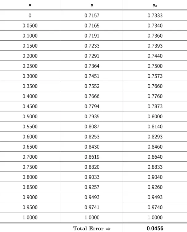
Hence forth, we will sample the total error with 21 mesh points. Tables 2.1 and 2.2 give the numerical comparison for different values of x.

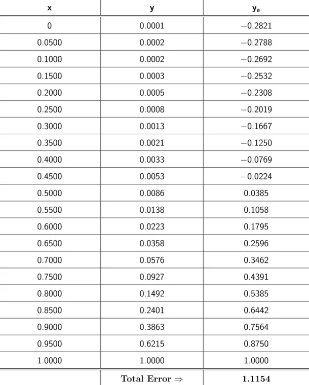
From Tables 2.1 and 2.2, we observe that the total error is high especially for

α = 10. From Figure 2.4 we notice that the error is unacceptably high. The solution which represents the concentration of the chemical becomes negative for

α = 10 and since this cannot happen in reality, we infer that more collocation points are needed to produce a higher degree approximation.

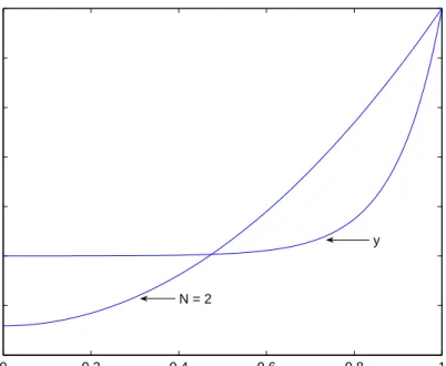
0 0.2 0.4 0.6 0.8 1 0.7 0.75 0.8 0.85 0.9 0.95 1 Distance, x Solution N = 2 y

Figure 2.1: Comparison ofy andya for Example2.5.1withα= 1and orderN = 2.

0 0.2 0.4 0.6 0.8 1 −18 −16 −14 −12 −10 −8 −6 −4 −2 0 2x 10 −3 Distance, x Error

0 0.2 0.4 0.6 0.8 1 −0.4 −0.2 0 0.2 0.4 0.6 0.8 1 Distance, x Solution y N = 2

Figure 2.3: Comparison of y and ya for Example 2.5.1 with α = 10 and order

N = 2. 0 0.2 0.4 0.6 0.8 1 −0.5 −0.4 −0.3 −0.2 −0.1 0 0.1 0.2 0.3 Distance, x Error

Figure 2.4: Error between y and ya for Example 2.5.1 with α = 10 and order

x y ya 0 0.7157 0.7333 0.0500 0.7165 0.7340 0.1000 0.7191 0.7360 0.1500 0.7233 0.7393 0.2000 0.7291 0.7440 0.2500 0.7364 0.7500 0.3000 0.7451 0.7573 0.3500 0.7552 0.7660 0.4000 0.7666 0.7760 0.4500 0.7794 0.7873 0.5000 0.7935 0.8000 0.5500 0.8087 0.8140 0.6000 0.8253 0.8293 0.6500 0.8430 0.8460 0.7000 0.8619 0.8640 0.7500 0.8820 0.8833 0.8000 0.9033 0.9040 0.8500 0.9257 0.9260 0.9000 0.9493 0.9493 0.9500 0.9741 0.9740 1.0000 1.0000 1.0000 Total Error _⇒ 0.0456

Table 2.1: Numerical comparison for one point collocation for Example2.5.1 with

x y ya 0 0.0001 ₋0.2821 0.0500 0.0002 ₋0.2788 0.1000 0.0002 ₋0.2692 0.1500 0.0003 ₋0.2532 0.2000 0.0005 ₋0.2308 0.2500 0.0008 ₋0.2019 0.3000 0.0013 ₋0.1667 0.3500 0.0021 ₋0.1250 0.4000 0.0033 ₋0.0769 0.4500 0.0053 ₋0.0224 0.5000 0.0086 0.0385 0.5500 0.0138 0.1058 0.6000 0.0223 0.1795 0.6500 0.0358 0.2596 0.7000 0.0576 0.3462 0.7500 0.0927 0.4391 0.8000 0.1492 0.5385 0.8500 0.2401 0.6442 0.9000 0.3863 0.7564 0.9500 0.6215 0.8750 1.0000 1.0000 1.0000 Total Error _⇒ 1.1154

Table 2.2: Numerical comparison for one point collocation for Example2.5.1 with

2.5.2

Generalization of Example

2.5.1

We can improve the accuracy of our approximation by increasing the number of collocation points but as the number of collocation points increases, the number of equations and unknowns also increases, thus making computation by hand very tedious. Thus we will first generalize the problem and reduce it to a linear system. We can then use any programming language with a high speed computer to solve for the unknowns.

In general, we substitute the approximate solution of the form (2.40) into the differential equation(1.19) to obtain

N+1 X k=1 h ckl ′′ k(x) +ckl ′ k(x)−α2cklk(x) i = 0. (2.49)

We first satisfy the left hand boundary condition atx1, then evaluate the residual

(2.49) at the collocation pointsxc

j ,j = 2, 3, ...,N, and finally satisfy the right hand

boundary condition at xN+1. The resulting linear system of equations can be cast

in the matrix vector form Ac = b, where A = aij is a (N + 1)×(N + 1) matrix

with a₁j = l ′ j(x1), (2.50) ai,j = l ′′ j (x c i ) +l ′ j(x c i )−α2lj(xic), (2.51) aN+1,j = lj(xN+1), (2.52)

for j = 1, 2, ...,N+ 1,i = 2, 3, ...,N, b is a column vector of dimension N + 1 with

bj = 0; j = 1, 2, ...,N, (2.53)

bN+1 = 1 (2.54)

and

c=cj; j = 1, 2, ...,N + 1, (2.55)

is the vector of the unknowns. Hence the solution vector isc=A−1b. This system has been coded in MATLAB and the code is given in Appendix A.

We first solve the problem by choosing the collocation points xc

j , j = 2, 3, ...,N

as the shifted roots of the Chebyshev polynomial of the first kind, TN−1. In this

instance we emphasize that the collocation points agree with the internal interpo-lation points, that is xc

j =xj for j = 2, 3, ...,N. The plots of the solutions and the

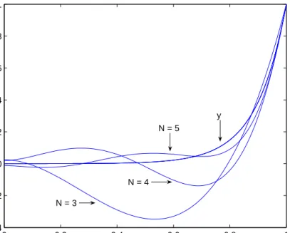
errors for ordersN = 3, 4 and 5 are given in Figures2.5 and 2.6 respectively. The case N = 16 is displayed in Figure 2.7.

In Table 2.3 we summarize the total error for different orders N. We notice the gradual decrease in the total error as we increase the order of the polynomial. The total error for orders N _≥ 9are small. If we use polynomials of ordersN = 16 and above, the error levels off at 3.1380e₋006.

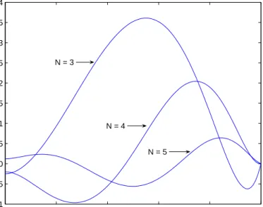
0 0.2 0.4 0.6 0.8 1 −0.4 −0.2 0 0.2 0.4 0.6 0.8 1 Distance, x Solution N = 3 N = 4 N = 5 y

Figure 2.5: Comparison of y and ya for Example 2.5.1 for ordersN = 3, 4, 5, with

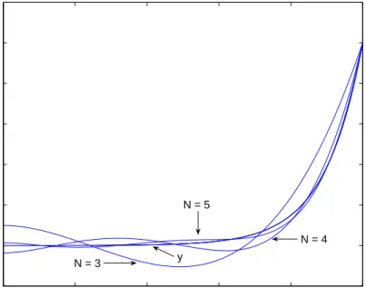
0 0.2 0.4 0.6 0.8 1 −0.1 −0.05 0 0.05 0.1 0.15 0.2 0.25 0.3 0.35 0.4 Distance, x Error N = 3 N = 4 N = 5

Figure 2.6: Errors for Example 2.5.1for orders N = 3, 4, 5, with collocation points chosen as the shifted roots of TN−1.

0 0.2 0.4 0.6 0.8 1 −1.6 −1.4 −1.2 −1 −0.8 −0.6 −0.4 −0.2 0x 10 −6 Distance, x Error

Figure 2.7: Error for order N = 16 for Example 2.5.1, with collocation points chosen as the shifted roots of T15.

Secondly we choose the collocation points as the shifted roots of the Chebyshev polynomial of the second kind, UN−1. The plots of the solutions and the errors for

orders N = 3, 4and 5are given in Figures 2.8 and 2.9 respectively.

Thirdly we choose the collocation points as the shifted roots of the Legendre poly-nomial, PN₋1. The plots of the solutions and the errors for orders N = 3, 4 and 5

are given in Figures 2.10 and 2.11 respectively.

Comparing the total error from Table 2.3, we observe that the total error is least forUN−1. However, in all cases due to truncation error, the total error levels off at

order N = 16 with value 3.1380e₋006.

0 0.2 0.4 0.6 0.8 1 −0.2 0 0.2 0.4 0.6 0.8 1 1.2 Distance, x Solution y N = 3 N = 4 N = 5

Figure 2.8: Comparison of y and ya for Example 2.5.1 for ordersN = 3, 4, 5, with

0 0.2 0.4 0.6 0.8 1 −0.2 −0.15 −0.1 −0.05 0 0.05 0.1 0.15 Distance, x Error N = 3 N = 4 N = 5

Figure 2.9: Errors for Example 2.5.1for orders N = 3, 4, 5, with collocation points chosen as the shifted roots of UN₋1.

0 0.2 0.4 0.6 0.8 1 −0.2 0 0.2 0.4 0.6 0.8 1 1.2 Distance, x Solution N = 3 N = 4 N = 5 y

Figure 2.10: Comparison ofy and ya for Example2.5.1 for ordersN = 3, 4, 5, with

0 0.2 0.4 0.6 0.8 1 −0.15 −0.1 −0.05 0 0.05 0.1 0.15 0.2 Distance, x Error N = 3 N = 4 N = 5

Figure 2.11: Errors for Example2.5.1for ordersN = 3, 4, 5, with collocation points chosen as the shifted roots of P_N−1.

Order N TN₋1 UN₋1 PN₋1 2 1.1154 1.1154 1.1154 3 0.9755 0.4047 0.4925 4 0.4908 0.1554 0.2406 5 0.1631 0.0568 0.0913 6 0.0460 0.0181 0.0277 7 0.0120 0.0051 0.0073 9 6.1817e₋004 2.9281e₋004 3.9050e₋004 11 2.3159e₋005 1.2620e₋005 1.5287e₋005 13 3.2087e₋006 3.1525e₋006 3.1684e₋006 15 3.1382e₋006 3.1379e₋006 3.1381e₋006 16 3.1380e₋006 3.1380e₋006 3.1380e₋006

Table 2.3: Numerical comparison of the errors for Example 2.5.1 for different orders N, with collocation points chosen as the shifted roots of TN−1, UN−1 and

Example 2.5.2 In order to investigate how well the collocation method can track a hump, we solve the following non homogeneous boundary value problem on the interval [0, 3.5]: d2y dx + 6 dy dx + 9y = e −3x_, y(0) = 0, y(3.5) = 9.625e−10.5. (2.56)

Note that in the previous example, we shifted the roots of the orthogonal polyno-mials from [₋1, 1]to the domain of the problem namely [0, 1]. Here we choose to transform the domain [0, 3.5] of the problem to the interval [₋1, 1] by using the linear transformation L :x _→2x/h₋1, where h= 3.5 is the length of the domain [0, 0.35]. With this transformation, the differential equation (2.56) together with its boundary conditions becomes

4 h2 d2_y dx2 + 12 h dy dx + 9y = e −1.5h(x+1)_, y(₋1) = 0, y(1) = 9.625e−10.5. (2.57)

The exact solution to equation (2.56) is given by

y(x) =xe−3x + 0.5x2e−3x. (2.58)

The exact solution in equation (2.58) has a maximum value at x _≈ 0.3874 and damps off quickly as illustrated in Figure2.12.

2.5.3

Two Points Collocation for Example

2.5.2

4

X

k=1