OpenSource GPS
Open Source Software for Learning about GPS
Clifford Kelley, University of Southern California, Joel Barnes, University of New South Wales
Jingrong. Cheng, University of California Riverside
BIOGRAPHY
Mr. Kelley holds a B.S. in Physics, a B.S. in Electrical Engineering, an M.S. in Systems Engineering, and is currently pursuing a Ph.D. in Industrial and Systems Engineering at USC. He has been working on GPS programs at Boeing as a Senior Engineering Specialist in the advanced systems engineering area since 1997. Joel Barnes holds a Satellite Geodesy Ph.D. from the University of Newcastle upon Tyne, UK. Since December 2000 he has been working as a postdoctoral research fellow with the SNAP group, in the School of Surveying & SIS, the University of New South Wales (UNSW), Australia. Joel's current research interests are high precision kinematic GPS positioning, Pseudolites and GPS receiver firmware customization.
Jingrong Cheng holds B.S & M.S degrees from Harbin Engineering University in China. She is currently a Ph.D. student of University of California, Riverside (UCR). Her research focuses on the Integration of INS & GPS, mainly about how to aid GPS receiver with external INS information.
ABSTRACT
Teaching the next generation of engineers about the inner workings of GPS receivers is difficult due to the expense of acquiring appropriate hardware and software. In the past few years a number of excellent books have been written about GPS (references 1 through 5). But, in the end students learn best by doing. Even with hardware available, trying to squeeze the development of software into a quarter or a semester is asking a lot. A low cost set of hardware, along with free open source software, allows students access to the inner workings of the receiver without 'breaking the bank' in terms of time or money. This article will present open source GPS receiver software and laboratory hardware that is a straightforward
modification of a COTS receiver to interface it to a PC bus.
The hardware and software are based on the GEC Plessey, then Mitel, now Zarlink, chipset. In the 1990’s GEC introduced a board and software called the GPS Builder ™ which placed the down converter and correlator chips on an ISA card installed on a PC. Since the software ran on the PC it gave the user complete control and visibility into the operation of the receiver. Unfortunately GEC and Mitel found that they had to charge in excess of $1000 dollars for the board and software licenses. This served to limit its popularity among cash strapped universities and individuals.
Given the success of Linux, it was apparent that complex software development could be done on free open source software. This paper describes the hardware and software architecture, the features added to allow debugging of the code and carrier tracking loops, and plans for improving the software, install it on other receiver hardware, use embedded ‘x86 hardware, and to run under Open Source real time operating systems. A comparison will also be made of the software using two receivers, and will show the results of its performance.
This is similar to experiments that students could perform using the open source software and hardware discussed herein. An Internet website has been set up at
http://www.home.earthlink.net/~cwkelley to describe the project, and to provide source code and sample input and output data.
HARDWARE
GPS receiver hardware is complicated by the fact that there is RF signal processing in close vicinity to digital signals, which can interfere with the RF signal chain. In 1995 a 2-sided board was designed and built based on the GP 2020 chipset, which had 6 channels per chip. While it was possible to get it to work it was obvious that it had problems resetting and limited functionality. Building
high quality 4 layer surface mount component boards is expensive and requires specialized test equipment. Another alternative was needed. While working with the
Canadian Marconi AllStarTM and SuperStarTM it was
noticed that it used the same chipset. Since the
SuperStarTM OEM board is relatively inexpensive and
well built it suggested the idea of “hacking” into the hardware to bypass the digital processing on the board, and connect directly into a PC. A description of how to do this is provided on the website. Since the SuperStarTM
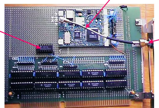
GP2021 interface is set up as a ‘186, the hardware was easy to setup. Although it destroys a perfectly good receiver, it seems to work well. Versions of the “hacked” receiver are working at both UCR and UNSW. Now, with hardware available for less than $200, adapting the software to the GP2021 was the only missing part. Figure 1 is a photograph of the hardware with the “hacked” receiver mounted to an ISA bus experimental card.
Figure 1
Photograph of “hacked” GPS receiver As shown in Figure 2, the receiver consists of an RF
"front end" chip and a digital processing chip connected to a PC I/O interface. The front end connects directly to the 10MHz clock and sends a 40MHz signal to the correlator chip. The correlator chip appears to the PC as a set of about 100 read and/or write registers. The RF signal is first down converted to about 175MHz, is sent to a simple band pass filter, and sent back to the front end. The second down converter stage is at about 35MHz. A SAW filter is used to filter and return the signal to the front end. In the final stage the signal is down converted to 4.3MHz and a 2-bit A/D converter (sign and magnitude) is used to transmit the signal information to
the GP2021 correlator chip. The correlator chip provides the sample timing, which is simply the 40MHz clock divided by 7. The PC interface consists of an ISA I/O board from JDR Electronics set up to address two 16-bit ports. One port (0x304) uses the lower 8 bits to send the register address. The other port (0x308) is used to read and write 16 bits of data. The correlator chip interface can be set up in a number of ways. As it is set up as an Intel 186 interface an indeterminate amount of time is available between latching the address and transferring the data.
7404
RF cable
MCX to SMA
SMA
bulkhead
adapter
Figure 2
Receiver Hardware Interface
SOFTWARE
OpenSource GPS is a C program written in Borland C (version 4.5 and later) without any embedded assembly language. As shown in Figure 3 the software uses a single interrupt routine to handle the tracking loops and find the navigation message. All other functions are handled using a polling method triggered by flags from the interrupt routine. Figure 4 shows the main software block diagram while Figure 5 illustrates in more detail the interrupt processing. In order to reduce connections to the correlator chip, the PC clock timing (interrupt 0) is taken over and is modified to provide an interrupt every 500 to 900µs.
Figure 3 Software Block Diagram
Figure 4 Main Program
Figure 5 Interrupt Routine
Figure 6 is a file structure diagram of the software. The program is written in three parts. GP2021 contains functions that deal with communication with the correlator chipset. The main routine is in gpsrcvr while gpsfuncs contains the library of GPS functions such as satellite location by using the almanac, ephemeris, computing the navigation solution and decoding the navigation message. The input file used only for input is the rcvr_par.dat file which contains constants used by the receiver, such as tracking loop constants for code and carrier for pull-in and tracking along with flags for various outputs. The input/output files are read at the start of the program and updated when the program exits. The output files record data for later analysis.
Main Program Interrupt Service Routine Enable PC Clock Interrupt Generator Common Variables/ Flags Input Files Output Files I/O Files 512 µs delay 512 µs delay Disable PC Clock Interrupt Generator Initialize Allocate channels Display Nav Fix Decode Nav Message Allocate channels Check Flags Start Start Ephemeris to ECEF Almanac to ECEF Exit? Exit? Exit Exit
Get Correlation data Get measurement data set nav flag, set allocate flag
Ch++ Search (1) Confirm (2) Pull -in (3) Chan state Track (4) Preamble Set Nav data flag Ch<12 Ch<12 Ch=0 Start Start Exit Exit
Figure 6
OpenSource Software File Structure
As seen in Figure 7, each channel provides 4 correlation counts. The prompt and dither (either ahead or behind the prompt correlator by 1/2 chip) both have in-phase "I" and quadrature "Q" correlators. By forming an RSS (root sum square) of the in-phase and quadrature values one can determine if they are lined up with the PRN code. The in-phase and quadrature correlator values indicate what the phase of the signal is. Although the source code includes comments, it is helpful to explain in more detail how the receiver software works.
Figure 7 Channel Block Diagram
To track the signal one does not directly 'move' the correlators, just speed up or slow down the carrier and code DCO's (digitally controlled oscillators) to keep the channel locked in code and carrier phase.
The correlator read timing of the receiver is set by taking over the PC's Int 0 which is normally used to keep the computer real time clock up to date. The 8254 normally interrupts the computer about every 50ms. This software replaces this interrupt routine with its own (GPS_interrupt) and sets the interrupt time to about 500µs. Whenever the interrupt occurs, the channel data register is checked to see which channels have dumped
correlation data. The correlator data is read and a check is made to see if a 99.9999 ms "tic" has occurred. If it has, the measurement data is stored. Each channel is processed based on the state the channel is in. Figure 8 shows the channel state diagram used.
Figure 8 Channel State Diagram
State 1 is the acquisition state. It does the code and frequency (Doppler) search to find a high correlation peak. If a peak in either the prompt or delay correlator (RSS of in-phase and quadrature) is above the threshold it switches to state 2. When in warm or cold start mode the Doppler is centered on the expected value. The search is conducted with two loops, the inner loop is the code search and the outer is the frequency search. The code search pattern is simply "slewing" the PRN generator by adding an extra chip of delay after each correlation sample. Thus after 1023 samples every 1/ 2 chip in code space has been searched. The frequency search pattern checks on either side of the expected frequency in integer multiples of the Doppler search range i.e. (0, +1, 1, +2, -2, ...)*200 Hz. The maximum range depends on what the receiver is doing. The nominal value is for a warm start, it is larger if attempting a cold start and smaller if the receiver has a navigation fix. Samples are taken every millisecond. This allows each frequency bin to be searched in about 1 second (if it does not go into state 2).
State 2 is the confirmation state. The confirmation state stops the search and dwells at the code and Doppler where the high correlation peak was found in state 1 to confirm the presence of the signal in order to reduce the false alarm rate. If n of m samples (e.g. 8 of 10) are above threshold it switches to state 3.
State 3 is the pull-in state. The signal has been confirmed but the frequency may be up to ~500Hz off. The pull-in state attempts to start tracking the signal in order to pull the frequency in close enough that the carrier phase can be tracked. In addition it should be noted that in order to reduce start-up transients the code loop is closed after 2ms and the carrier loop is closed after 5ms. This state is enabled for about 1500ms, during the last 500ms of this
1 Search 2 Confirm 3 Pull-in 4 Track
Code & Phase Track? n of m > threshold?
Prompt or Delay > threshold?
C/No < Threshold? Carrier DCO I Q 1 ms Epoch 20 ms Epoch Code DCO PRN Generator Prompt Dither * = Binary multiplier From Down converter 2 * * Integrate Dump * * * * * * * * * * Prompt_I Prompt_Q Dither_I Dither_Q gpsrcvr.cpp gpsfuncs.cpp gp2021.cpp gpsrcvr.cpp gpsfuncs.cpp gp2021.cpp
Input Files Output Files
Input/Output Files
current.alm current.eph ion_utc.dat curloc .dat
Program Files
rcvr_par.dat
Gpsrcvr.log
time the C/No and phase errors are measured and the program attempts to synchronize onto the edge of a data bit. If it confirms carrier and code tracking it switches to state 4. Since the frequency is likely to be very far off, the receiver uses a combination of a frequency locked loop FLL and a phase locked loop PLL. As the time progresses into the state the effect of the FLL is decreased so that at the end of the state the PLL is dominant. Figure 9 shows the pull-in carrier tracking block scheme.
Figure 9
Second Order PLL with Frequency Aiding
The filter is a second order PLL with first order frequency error aiding. The nature radian frequency
ω
of of the FLL is different from the nature radian frequencyω
op. These natural frequencies are determined by the desired loop filter noise bandwidthB
nf andB
np respectively. These values have the following relationship:v For the second order PLL:
B
np op=
1
.
89
ω
ω
ω
op opa
2=
1
.
414
v For the first order FLL:
B
nf of=
4
ω
The transfer function of the loop filter is:
)
(
)
(
)
(
)
(
2 2s
f
s
s
p
s
s
ω
opa
ω
opω
ofω
=
+
+
Rearranging:)
(
)
(
)
(
)
(
s
2s
2p
s
f
s
s
×
ω
=
a
ω
op+
ω
op×
+
ω
of×
Expressing this in time domain gives:
f
p
dt
dp
dt
d
of op opa
×
+
×
+
×
=
ω
ω
ω
ω
2 2f
p
f
op of opa
×
+
×
+
×
=
ω
ω
2ω
2Over a sample interval T:
T
n
n
dt
d
ω
=
ω
(
)
−
ω
(
−
1
)
,T
n
p
n
p
dt
dp
n
f
(
)
=
=
(
)
−
(
−
1
)
Therefore:)
(
2
)
(
)
2
(
)
1
(
)
(
n
−
ω
n
−
=
a
ω
op
+
ω
of
T
×
f
n
+
ω
op
T
×
p
n
ω
More conveniently:)
(
2
)
(
)
2
(
)
1
(
)
(
n
=
ω
n
−
+
a
ω
op
+
ω
of
T
×
f
n
+
ω
op
T
×
p
n
ω
The initial
ω
, the initial carrier NCO in the PULL_INroutine, is the data from search. When implementing these in software one should consider the carrier NCO resolution.
A four-quadrant arctangent
ATAN
2
(
Q
ps,
I
ps)
is usedas phase detector:
)
,
(
2
Q
I
ATAN
ps ps =Phase-errorp
+b
(
t
)
×
π
, where)
(
t
b
=0 or 1 So=
)
(
n
p
ATAN
2
(
Q
ps,
I
ps)
-b
(
t
)
×
π
Frequency error:T
n
p
n
p
n
f
(
)
=
(
)
−
(
−
1
)
whereT
=
1
ms
The figures below are actual data from a pull-in attempt and illustrate how it works. In Figure 10 it can be seen that the phase is changing rapidly at the start. As time progresses to about 200ms the phase is changing more slowly. By the time one gets to about 300ms it is close to phase lock. From this point on one can see the data bits as +90 and -90 degree phase transitions.
Figure 10
Carrier Phase During Pull-in -200 -100 0 100 200 1 101 201 301 401 501 601 701 801 901 1001 1101 1201 1301 1401 Time (ms) Phase (deg) Phase Error p Frequency Error f Update to NCO ω 1 s
ω
ofω
2 opa
2ω
op NCOIn Figure 11 one can see the noise in the carrier-tracking loop. It starts out high (due to the FLL) and transitions down in three steps every 500ms. At the end the effect of the FLL is negligible and the PLL dominates.
Figure 11
Carrier DCO Settings During Pull-in
Figures 12 and 13 show the code loop performance during pull-in. The beginning transient can be seen in figure 12 and within 400 ms the loop has stabilized. Figure 13 shows that the code DCO settings also indicate this initial transient and subsequent settling.
Figure 12
Prompt and Dither Magnitudes during Pull-in
Figure 13
Code DCO Settings During Pull-in
State 4 is the normal tracking state. The tracking loops are aligned with and integrate over a data bit (20ms) to track code and 1ms to track phase. The data message is recorded and the time is synchronized to the TOW (time of week) of the data message. Figure 14 illustrates the BPSK nature of the data recovered by the tracking loop.
Figure 14
Data Bits in Tracking Loop
To reduce the code tracking noise the code-tracking loop is aided by the carrier-tracking loop. Figure 15 shows the scaled error signal during tracking. It shows no sign of bias.
Figure 15
DLL Scaled tracking error During Tracking Figure 16 shows the carrier DCO during tracking. This is provided to the tracking loop where it is divided by 1540, the ration of the PRN code length to the wavelength of L1. 32975000 32980000 32985000 32990000 1 101 201 301 401 501 601 701 801 901 1001 1101 1201 1301 1401 Time (ms)
Carrier loop freq
-30000 -20000 -10000 0 10000 20000 30000 -30000 -20000 -10000 0 10000 20000 30000
Inphase Correlation
Quadrature Correlation
0 200 400 600 800 1000 1200 1400 1600 1800 1 101 201 301 401 501 601 701 801 901 1001 1101 1201 1301 1401 Time (ms) Correlation Magnitude Prompt Dither 24027500 24028000 24028500 24029000 24029500 24030000 1 101 201 301 401 501 601 701 801 901 1001 1101 1201 1301 1401 Time (ms) Frequency Count -6000 -4000 -2000 0 2000 4000 6000 0 500 1000 1500 Data Bits Scaled ErrorFigure 16
Carrier DCO During Tracking
Figure 17 illustrates the extremely tight tracking of the code loop as it spends its time alternating between 2 code DCO setting for the majority of the time.
Figure 17
Code DCO During Tracking
By following the space segment to user segment ICD-GPS-200 (Interface Control Document) see reference 7 the navigation message can be interpreted and a navigation fix in position, velocity and time can be computed. In order to provide accuracies on the order of a few meters all of the corrections must be made. These include the Sagnac effect, relativistic effects and troposphere and ionosphere models. In order to determine if these algorithms were correctly applied and provide a way to debug the program a comparison with a commercial receiver using the same chipset was performed.
RECEIVER COMPARISON
The operation of OpenSource GPS was compared to a
CMC AllstarTM. The test was conducted at UNSW by
splitting the signal from an antenna to the AllstarTM and a PC running the OpenSource software on a “hacked” receiver. Since both use the same receiver chipset the
only differences should be due to the software. The antenna location at UNSW has been surveyed so that an absolute error can be computed. As seen in figures 18 and 19 the number of satellites matches for only brief periods of time. The VDOP, and HDOP matched closely over most of the data set but also of course show differences when the number of satellites used is different.
0 1000 2000 3000 4000 5000 6000 7000 8000 0 2 4 6 8 10 12 No SVs HDOP VDOP Figure 18
No. of SVs, VDOP, HDOP vs Time, AllstarTM
0 1000 2000 3000 4000 5000 6000 7000 8000 0 2 4 6 8 10 12 No SVs HDOP VDOP Figure 19
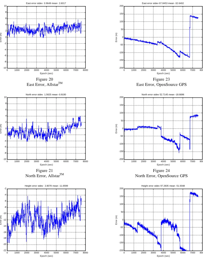
No. of SVs, VDOP, HDOP vs Time, OpenSource GPS Figures 20 through 22 present the time histories of east error, north error, and height error respectively for the AllstarTM receiver. Figures 23 through 25 also present the time histories of east error, north error, and height error respectively for the OpenSource GPS receiver.
33035000 33035200 33035400 33035600 33035800 33036000 33036200 0 500 1000 1500 Data Bits Carrier DCO 24028310 24028311 24028312 24028313 24028314 24028315 0 500 1000 1500 Data Bits Code DCO
0 1000 2000 3000 4000 5000 6000 7000 8000 -10 -8 -6 -4 -2 0 2 4 6 8 10
East error stdev 0.9649 mean 2.6017
Error (m)
Epoch (sec)
Figure 20 East Error, AllstarTM
0 1000 2000 3000 4000 5000 6000 7000 8000 -10 -8 -6 -4 -2 0 2 4 6 8 10
North error stdev 1.5625 mean -0.9190
Error (m)
Epoch (sec)
Figure 21 North Error, AllstarTM
0 1000 2000 3000 4000 5000 6000 7000 8000 -22 -20 -18 -16 -14 -12 -10 -8 -6 -4 -2
Height error stdev 2.8078 mean -11.6599
Error (m)
Epoch (sec)
Figure 22 Height Error, AllstarTM
0 1000 2000 3000 4000 5000 6000 7000 8000 -200 -150 -100 -50 0 50 100 150 200
East error stdev 67.8453 mean -32.6402
Error (m)
Epoch (sec)
Figure 23
East Error, OpenSource GPS
0 1000 2000 3000 4000 5000 6000 7000 8000 -200 -150 -100 -50 0 50 100 150 200
North error stdev 52.7145 mean -18.6696
Error (m)
Epoch (sec)
Figure 24
North Error, OpenSource GPS
0 1000 2000 3000 4000 5000 6000 7000 8000 -200 -150 -100 -50 0 50 100 150 200
Height error stdev 97.2835 mean -51.9348
Error (m)
Epoch (sec)
Figure 25
Height Error, OpenSource GPS
Figures 26 and 27 illustrate the accuracy of the navigation
solutions from each receiver. While the AllstarTM
dispersion of about 2m in radius, the OpenSource GPS software has a large bias change when a new set of satellites is used in the solution. In addition the solution gradually drifts during a fixed set of satellites. The dispersion, when the solution remains stable is about 10 meters. -10 -8 -6 -4 -2 0 2 4 6 8 10 -8 -6 -4 -2 0 2 4 6 Horizontal Error
East (m) stdev 0.9649 mean 2.6017
North (m) stdev 1.5625 mean -0.9190
Figure 26
Position Fix Error, AllstarTM
-200 -150 -100 -50 0 50 100 150 200 -150 -100 -50 0 50 100 Horizontal Error
East (m) stdev 67.8453 mean -32.6402
North (m) stdev 52.7145 mean -18.6696
Figure 27
Position Fix Error, OpenSource GPS
Current Work
From the data presented it is obvious that much more work needs to be done. The basic functionality of the software has been tested but the navigation algorithms need more testing and debugging.
Since beginning in early 2001 the website has been visited by approximately 10000 people. A number of students and researchers worldwide have studied OpenSource GPS software, and a few have “hacked” hardware. This collaboration has already found a number of errors and
improved the code immensely. It is expected that, as more people become involved, the quality of the software and availability of hardware will improve to the point that anyone with an interest in GPS can, for less than $200, set up their own GPS lab.
Areas for Improvement/Plans for the Future
Obviously no program is perfect, especially when written on one's own time without access to sophisticated test equipment. While it appears to work pretty well there are a number of areas where there are problems, and other areas where it could be greatly improved:
• Fixing the problems with the position fix
routines
• The acquisition/pull-in steps integrate over 1ms,
a longer integration time or variable integration time may be desirable.
• The tracking loops currently integrate over 20ms,
a longer integration time or variable integration time may be desirable.
• The C/No computation appears to be in error
(possibly a few dB low?).
• Velocity is derived from the carrier tracking
loops not from carrier phase measurements. The code and carrier tracking loops are only 2nd order and could be much better.
• There is no Kalman filter in the program.
Any comments or suggestions are most welcome. Please direct them to Mr. Kelley at [email protected].
Acknowledgements:
The authors would like to acknowledge the encouragement of Jay Farrell at UCR, and the interest of Chris Rizos and Jinling Wang from UNSW. In addition Georg Beyerle has done quite a bit of work adapting the software for a PCI interface card and has created a Linux version of the software (see reference 10).
References:
1. Kaplan, Elliott D. ed. 1996. Understanding GPS:
Principles and Applications. Boston: Artech House Publishers.
2. Misra, Pratap, Enge, Per 2001, Global
Positioning System Signals, Measurements, and Performance, Ganga-Jamuna Press
3. Hoffmann-Wellenhof, B. H., Lichtenegger, and J. Collins. (1994). GPS: Theory and Practice. 3rd ed. New York: Springer-Verlag.
4. Parkinson, Bradford W. and James J. Spilker.
eds. (1996). Global Positioning System: Theory and Practice. Volumes I and II. Washington, DC: American Institute of Aeronautics and Astronautics, Inc.
5. Tsui, James B.-Y, (2000). Fundamentals of
Global Positioning System Receivers, A Software Approach. John Wiley & Sons
6. Zarlink, (2001). GP2021 Data Sheet,
http://www.zarlink.com
7. GPS Joint Program Office, 1997. ICD-GPS-200:
GPS Interface Control Document. ARINC Research. Available on line from the United States Coast Guard Navigation Center.