PYROLYSIS-GAS CHROMATOGRAPHY-

A

LMA

M

ATER

S

TUDIORUM

-U

NIVERSITY OF

B

OLOGNA

D

EPARTMENT OF

C

HEMISTRY

“G.

C

IAMICIAN

”

Ph. D.

COURSE

IN

C

HEMICAL

S

CIENCE

C

XXIV

Afference sector: CHIM/03A1

Scientific-disciplinary sector: CHIM/01

P

YROLYSIS

-

GAS CHROMATOGRAPHY

-MASS SPECTROMETRY AND

CHEMOMETRIC ANALYSIS FOR THE

CHARACTERIZATION OF

COMPLEX MATRICES

Presented by

S

M

School doctorate coordinator Advisor

Prof.

A

B

Prof.

D

M

1

2

INTRODUCTION ... 4

SECTION A THEORY ... 7

CHAPTERA1 ANALYTICAL PYROLYSIS ... 8

A1-1 Introduction to analytical pyrolysis ... 9

A1-2 Degradation mechanisms ... 11

A1-3 The integrated system Py-GC-MS ... 14

A1-4 Derivatization ... 20

CHAPTER A2 MULTIVARIATE DATA ANALYSIS ... 23

A2-1 Introduction to chemometrics ... 24

A2-2 Multivariate structure data ... 26

A2-3 Data pretreatment ... 27

A2-4 Principal component analysis ... 30

A2-4.1 Introduction ... 30

A2-4.2 The principal components ... 30

A2-4.3 Loading and score plots ... 33

A2-4.4 Geometric interpretation of PCA ... 35

A2-4.5 The number of significant components ... 37

A2-5 SIMCA (Soft Independent Modeling of Class Analogy) ... 39

A2-5.1 SIMCA Class-Models ... 40

A2-5.2 Statistical Significance Level in SIMCA ... 42

A2-5.3 The Coomans Plot ... 42

SECTION B APPLICATIONS ... 44

CHAPTER B1 BEHAVIOUR OF PHOSPHOLIPIDS IN ANALYTICAL REACTIVE PYROLYSIS* ... 45

B1-1 Keywords ... 46

B1-2 Summary... 46

B1-3 Introduction ... 46

B1-4 Materials and Methods ... 48

B1-5 Results and discussion ... 50

B1-5.1 Pyrolysis-methylation ... 50

B1-5.1.1 Analysis of standard phospholipids ... 50

B1-5.1.2 Analysis of standard painting layers ... 52

B1-5.2 Pyrolysis-silylation ... 54

B1-5.2.1 Analysis of standard phospholipids ... 54

B1-5.2.2 Analysis of standard painting layers ... 55

B1-6 Conclusions ... 57

CHAPTERB2 MULTIVARIATE METHODS FOR EXPERIMENTAL-DATA ANALYSIS APPLIED TO IDENTIFICATION OF BACTERIA BY MEANS OF PY-GC-MS ... 59

B2-1 Summary... 60

3

B2-3 Introduction ... 61

B2-4 Materials and methods ... 62

B2-4.1 Bacteria samples ... 62

B2-4.1.1 Preparation of Bacillus samples ... 62

B2-4.1.2 Preparation of Pseudomonas samples ... 63

B2-4.1.3 Preparation of Rhodococcus samples ... 64

B2-4.2 Experimental conditions ... 65

B2-5 Results and discussion ... 67

B2-5.1 Identification of pyrolysis compounds ... 67

B2-5.2 Reproducibility ... 70

B2-5.3 Distinction between bacterial genera ... 71

B2-5.4 Distinction between bacterial species of Bacillus ... 72

B2-5.4.1 Chemometric analysis ... 72

B2-5.4.1.1 Principal Components Analysis ... 73

B2-5.4.1.2 SIMCA classification ... 76

B2-5.5 Distinction between bacterial species of Pseudomonas ... 77

B2-5.5.1 Chemometric analysis ... 78

B2-5.5.1.1 Principal Components Analysis ... 79

B2-5.5.1.2 SIMCA classification ... 81

B2-5.6 Effect of culture conditions: analysis of Rhodococcus Aetherovorans BCP1 ... 82

B2-5.6.1 Chemometric analysis ... 83

B2-5.6.1.1 Principal Components Analysis ... 84

B2-5.6.1.2 SIMCA classification ... 87

B2-6 Conclusions ... 88

CHAPTERB3 CHARACTERIZATION OF A MIXED-BIOFILM BY MEANS PY-GC-MS... 90

B3-1 Summary ... 91

B3-2 Keywords ... 91

B3-3 Introduction ... 91

B3-4 Materials and methods ... 93

B3-4.1 Preparation of microorganisms for the growth in biofilms ... 93

B3-4.2 Experimental conditions ... 94

B3-5 Results and discussion ... 96

B3-5.1 Analysis of bacterial and fungal biofilms ... 96

B3-5.2 Analysis of mixed-biofilm ... 99

B3-6 Conclusions ... 100

REFERENCES ... 102

4

5

Analytical pyrolysis is a powerful technique for rapid analysis of complex and heterogeneous

organic materials, based on controlled thermal degradation of the sample in inert atmosphere. The organic material is either degraded to lighter neutral molecules or flash vaporized when thermally stable and volatile. Identification of pyrolysis products is obtained by retention times and mass spectra after coupling pyrolysis with gas chromatography and mass spectrometry (Py-GC-MS). Even though this is a destructive method, a single analysis with a minute amount of sample (less than 1 mg), without preliminary pre-treatment, is capable to provide information on a wide range of organic materials difficult to be analyzed by other methods. Py-GC-MS is extensively applied in the field of cultural heritage, environmental science, forensics and others.

The present PhD thesis was focused on the development and application of chemical methodology and data-processing method, both by classical univariate statistics and by multivariate data analysis (chemometrics). The chromatographic and mass spectrometric data obtained with this technique are particularly suitable to be interpreted by chemometric techniques such as principal component analysis (PCA), and classification techniques.

As a first approach, some issues related to the field of cultural heritage were discussed with a particular attention to the differentiation of binders used in pictorial field. In particular, it was possible to determine as a marker of egg tempera the phosphoric acid esterified, a pyrolysis product of lecithin. The analyses were carried out both on phospholipids standards either on painting standard layers prepared by the Opificio delle Pietre Dure (Florence, Italy).

The best results were obtained using as a derivatizing reagent the HMDS (hexamethyldisilazane) rather than the TMAH (tetramethylammonium hydroxide).

Recently, the interest in the use of analytical pyrolysis to study biological samples greatly increased. The validity of analytical pyrolysis as tool to characterize and classify different types of bacteria was verified.

Fatty acids represent the main organic compounds present in the structure of the wall bacterial cell; their chemistry is extremely variable because of the differences in chains length, the presence or absence of unsaturated groups and branched chains and hydroxylated groups. The fatty-acids chromatographic profiles represent an important tool for the bacterial identification.

Because of the complexity of the chromatograms, it was possible to characterize the bacteria only according to their genus, while the differentiation at the species level has been achieved

6

by means of chemometric analysis. To perform this study, normalized areas peaks relevant to fatty acids were taken into account. Chemometric methods such as PCA (Principal Component Analysis) and SIMCA (soft independent models of class analogy) were applied to experimental datasets. The obtained results demonstrate the effectiveness of analytical pyrolysis and chemometric analysis for the rapid characterization of bacterial species.

Application to a samples of bacterial (Pseudomonas Mendocina), fungal (Pleorotus ostreatus)

and mixed-biofilms was also performed. A comparison with the chromatographic profiles obtained from different biofilms was carried out and it was verified the possibility to:

• Differentiate the sample according to the fatty acid profile

• Characterize the fungal biofilm by means the typical pattern of pyrolytic fragments derived from saccharides present in the fungal structure

7

8

CHAPTER

A1

ANALYTICAL

9 A1-1 Introduction to analytical pyrolysis

Pyrolysis is defined as a chemical degradation reaction caused by thermal energy alone and

carried out in an inert atmosphere [1, 2]. The term chemical degradation refers to the decompositions and eliminations that occur in pyrolysis with formation of primary fragments, molecules of lower mass arising from the direct breaking of bonds of the analyte molecules, and secondary fragments of higher mass, resulting from intermolecular reactions between substrate and the primary products not yet degraded. The pyrolytic fragmentation is analogous to the processes that occur during the production of a mass spectrum: the energy supplied determines the breaking of the molecules into stable fragments. The pyrolytic reactions usually take place at temperatures between 500 ° C and 800° C; the chemical transformations taking place under the influence of heat at a temperature between 100°C and 300° C are called thermal degradations and not pyrolysis.

Analytical pyrolysis [3, 4] is by definition the characterization of a material by chemical

degradation reactions induced by thermal energy, while the pyrolysis itself is just a process that allows the transformation of the sample into other compounds. The pyrolytic process is carried out in a pyrolysis unit (pyrolyzer) interfaced with the analytical instrumentation. It is also possible to perform "off line" pyrolysis (no direct interface analytical instruments), followed by the analytical measurement. The pyrolyzers have a source of heat where the sample is pyrolyzed and the products are usually swept by a gas flow from the pyrolyzer to the analytical instrument. Pyrolysis can be performed in different modes: flash pyrolysis (pulse mode), slow gradient heating pyrolysis (continuous mode), step pyrolysis, etc. Usually, the pyrolysis for analytical purposes is carried out in “pulse mode”, that consists in a very rapid heating of the sample from ambient temperature, targeting isothermal conditions at a temperature where the sample is completely pyrolyzed. There is a fairly wide array of commercially available instruments for performing pyrolysis; most of them are designed primarily for the use with gas chromatographs. Microfurnaces provide a constantly heated, isothermal pyrolysis zone into which samples are introduced by a liquid syringe, solid plunger syringe or in a little cup. Curie-point pyrolyzers apply the sample to a piece of ferromagnetic metal which is inserted into the pyrolyzer when cold, then heated rapidly through induction of current using a high frequency coil. Depending on the metal alloy used, when it reaches a characteristic temperature (the Curie-point of that metal) no more current can be induced, so the temperature stops at that point. Filament style pyrolyzers use a piece of resistive metal

10

(frequently platinum) with a wide temperature range and circuitry capable of heating the filament up to a programmed temperature at controlled rate.

The production of smaller molecules from some larger favored the use of pyrolysis as a sample preparation technique, extending the applicability of instrumentation designed for the analysis of gaseous species to solids, especially polymeric materials. Polymers are not volatile and some of them are hardly soluble in common solvents and some decompose easily during heating.

The direct application of powerful analytical tools such as gas chromatography-mass spectroscopy (GC-MS) to most polymers and many complex materials is not feasible. Pyrolysis of these kinds of samples (polymers, composite organic materials) generates, in most cases, smaller molecules. The characterization of the pyrolytic fragments is performed by coupling the pyrolyzer to analytical methods such as gas chromatography, (Py-GC, Pyrolysis-Gas Chromatography), mass spectrometry (Py-MS, Pyrolysis-Mass Spectrometry), or more sophisticated integrated Py-GC-MS (Pyrolysis-Gas Chromatography-Mass Spectrometry). In these systems, the sample is heated to a temperature causing the rupture of the bonds and fragments are separated and recorded by an analyzer that provides the characteristic pyrolysis profile. This profile, called pyrogram, under suitable and controlled experimental conditions, can be considered a sort of finger-print of the substrate, both as regards the appearance of characteristic fragmentation products and for the distribution and relative concentration of these. It is an indirect characterization as it determines the composition of the substrate from the analysis of the fragments.

The advantages encountered by the application of the technique are numerous:

• Reduced time analysis

• No sample pre-treatment

• Small sample amount (lower than mg)

• Analysis of complex matrices

The major disadvantage is that the pyrolysis is a destructive technique, but this negative aspect is mitigated by the fact that only small amounts of sample are necessary: 0.1 mg for standard samples and 0.5 mg for others.

11

Analytical pyrolysis is frequently considered specific for polymers analysis, which may at first seem fairly limited. In fact, many compounds belong to this class, such as that proteins, polysaccharides, plastics, adhesives, paints, etc... natural and synthetic polymers, in the forms of textile fibers, wood products, foods, leather, paints, varnishes, plastic bottles and bags, and paper and cardboard, are materials that are part of daily life. Consequently, the study of these materials by pyrolysis has become a very broad field, including diverse topics such as soil nutrients, plastic recycling, criminal evidence, bacteria and fungi, fuel sources, oil paintings, and computer circuit boards.

A1-2 Degradation mechanisms

The pyrolysis products reflect the molecular structure, stability, free radicals, substitution and internal rearrangements of the polymers constituting the original sample. Identical molecules that undergo the same pyrolysis conditions degrade in the same characteristic way. The thermal degradation that a polymeric material undergoes when subjected to pyrolysis is characterized by breaking of chemical bonds and formation of free radicals. The way in which a molecule degrades depends on the type of bonds involved and on the stability of smaller fragments that are formed. These products, identified by GC-MS, can provide a fingerprint of the original polymer composition and microstructure and may help to determine the mechanisms of degradation.

The three main mechanisms include random scission, side-group scission, and monomer

reversion.

Random scission involves the random breaking of the polymer's C-C bonded backbone as all the bonds are of equal strength, resulting in the formation of products including, alkanes, alkenes and alkadienes of smaller sizes. The polyolefins are good examples of materials that behave in this manner (Figure A1-1).

12

Chain scission produces hydrocarbons with terminal free radicals which may be stabilized in several ways. If the free radical extracts a hydrogen atom from a neighboring molecule, it becomes a saturated end and creates another free radical in the neighboring molecule which may be stabilized in a number of ways. The most probable way is beta scission, which accounts for most of the polymer backbone degradation by producing an unsaturated end and a new terminal free radical. This process continues producing hydrocarbon molecules that are saturated and have one terminal double bond or a double bond at each end. When analyzed by gas chromatography, the resulting pyrolytic profile presents a series of triplet of peaks corresponding to the diene, alkene, and alkane containing a specific number of carbons and eluting in that order.

Side-group scission occurs when the side groups attached to the backbone are broken away resulting in the backbone becoming polyunsaturated. An example of a polymer which undergoes this type of degradation is poly (vinyl chloride) (PVC). A two-step degradation mechanism begins with the elimination of HCl from the polymer chain leaving a polyunsaturated backbone that, upon further heating, produces the characteristic aromatics which can be individuated in the pyrogram (Figure A1-2).

13

Monomer reversion results in unzipping and reverting back of the polymer to its original monomeric version. Polymers which are known to undergo this mechanism include

polymethylmethacrylate polytetrafluoroethylene, poly-α_{-methylstyrene and}

polyoxymethylene. This proceeds in copolymers as well, with production of both monomers

in roughly the original polymerization ratio (Figure A1-3).

14

Predicting the degradation mechanism of a polymer is not always immediate but is very useful. It can be achieved by three simple rules:

• Pyrolysis degradation mechanisms are free-radical processes and are initiated by breaking the weakest bonds

• The composition of the pyrolysate will be based on the stability of the free radicals involved and on the stabilities of the products.

• Free radical stability follows the usual order oforder 3°>2°>1°>CH3

A1-3 The integrated system Py-GC-MS

To perform an analysis by pyrolytic techniques, a system is required capable of heating small samples to pyrolysis temperatures in a reproducible way, interfaced to an instrument able to analyze the pyrolysis fragments produced. Pyrolysis-gas chromatography/ mass spectrometry is the integrated system mostly used to perform analytical pyrolysis.

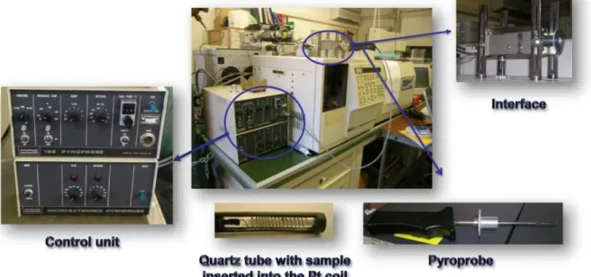
In Figure A1-4 the integrated system Py-GC-MS used in this work is reported:

15

The pyrolyzer, a heated filament pyrolyzer, can be considered as a sample introduction device; it’s directly connected to the injection port of a gas chromatograph and the pyrolysis fragments are sent with the flowing gas to the chromatographic column. Indeed, a flow of inert gas (helium) crosses the whole system ensuring an inert atmosphere in the pyrolyzer interface and acting as a carrier gas for the gas chromatographic separation of pyrolysis fragments (Figure A1-5).

Probe insert

Heating housing of the pyrolyzer

Heating coil

Sample holder

Inlet of the gas carrier

Outlet to GC injector

Figure A1-4 the integrated system Py-GC-MS

16

The pyrolyzer is constituted by a control unit connected to a cylindrical metal probe, to whose end a platinum coil resistance is mounted; inside the coil a capillary of quartz containing the sample is introduced, closed at the ends by quartz wool. The so obtained probe is inserted within the metal interface, which is mounted directly on the injector of the gas chromatograph, which is kept heated to an appropriate temperature (Figure A1-6).

The parameters used in the pyrolyzer must be set taking into account both the chromatographic performance and the proper sample degradation.

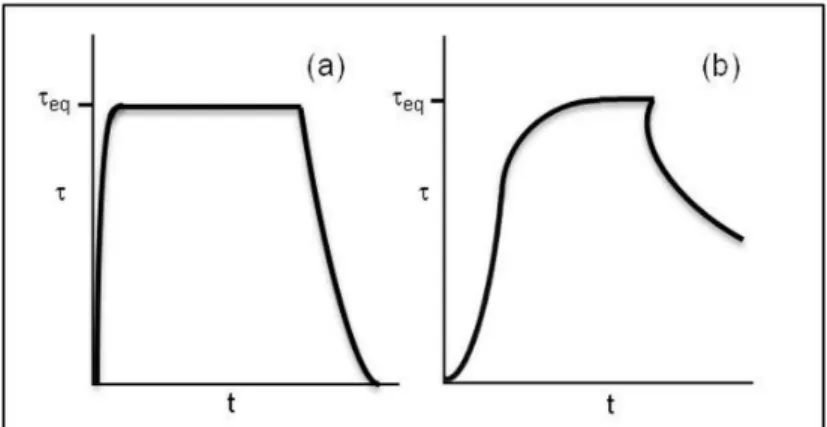
The control unit of the pyrolyzer is able to provide a strong electric pulse to the platinum resistance, which thus reaches the programmed temperature pyrolysis (TPY, Pyrolysis Temperature). The filament temperature may be monitored using the resistance of the material itself or some external measure, such as a thermocouple. The time taken by the pyrolyzer to reach the TPY set (TRT, Temperature Rise Time) must be extremely fast, with respect to the degradation temperature of the sample (flash pyrolysis). If the temperature raises too slowly the sample may pyrolyzes before reaching the programmed TPY and the primary fragments formed can, subjected to heating, recombine in a non-reproducible way (Figure A1-7).

17

As for gas chromatographic conditions, the pyrolysate pass through the injector when already volatilized; if the sample is heated slowly, or to a temperature at which degradation is slow, the volatiles will travel to the column over a finite time, which may produce peaks too broad to achieve the needed chromatographic resolution.

Pyrolysis temperature is maintained for a programmable short time interval (usually 10 s). Its value must be maintained between 400 ° C and 900 ° C since, above this range of values, fragments could be formed which are too small and not significant enough to characterize the original sample. The final distribution of pyrolysis fragments, or finger-print, is strongly influenced by pyrolysis temperature, which strongly influences the fragmentation reactions. The parameters TPY and TTP are that the ones mostly affecting reproducibility, together with the interface temperature (Tint). This temperature is kept high and constant ( about 250 °C) to

limit as much as possible any phenomena of condensation of pyrolytic fragments and to maintain the latter in the gaseous state to allow the transport by the mobile phase gas (carrier gas) through the gas chromatographic column. The interface should have a small internal volume to avoid fragments spending too much time in the zones not covered by gas flow, to reduce the contact between analytes and hot surfaces and to transfer pyrolytic fragments away from the high temperature zone (where secondary pyrolysis could take place) and into the column efficiently. The thermal fragmentation, inside the interface, takes place in an inert atmosphere (helium) to avoid the presence of oxygen, which would cause secondary reactions of oxidation and / or combustion.

Figure A1-7 TRT, temperature rise time a) Ideal condition; b) Poor condition for instrumental performance

18

It is appropriate to use a reasonable carrier flow (60 ml min-1): the greater the time past in the high temperature zone, the greater the possibility that secondary pyrolysis reactions take place.

The transfer zone between pyrolyzer and the GC injection port should be kept hot to prevent condensation, and as short as possible to reduce surface area and volume.

The sample should be very small to prevent phenomena such as the overloading of the pyrolyzer and analytical device, causing contamination and carryover into the next analysis. Small amounts of sample are degraded more rapidly and completely, ensuring good resolution and reproducibility. When it is not possible to limit the amount of sample, the use of an injection port with a splitter and a relatively high split ratio are suggested.

Sample preparation must be carefully performed, taking into account size and shape, homogeneity and contamination. If a sample material is soluble, a few microliters of the solution may be injected directly into the quartz wool inserted in the capillary, using a syringe. Usually, analytical pyrolysis is used for direct analysis of solid samples: this is surely its strength. But a very important issue that emerges when solid samples of a few micrograms are analyzed is how they are representative of the material from which they were taken. It is very common to handle non-homogeneous materials, natural or synthetic, and some precautions have to be taken not to compromise the reproducibility of the analysis:

• reducing the sample to a fine powder, and take small amounts of this

• dissolving the sample when its components are soluble

• analyzing an amount of sample as great as possible

In the last case, the use of a splitter with a large split ratio it’s suggested to limit the amount of the pyrolysate entering the analytical device. These are several ways to obtain a representative sample and ensure the reproducibility of the pyrolytic analysis.

In GC-MS, the gas flow-rate is commonly set between 0.1 to 3.0 mL/min (at near atmospheric pressure). Because the mass spectrometer operates at 10-5 to 10-7 mbar, it is equipped with efficient pumps, which maintain high vacuum inside.

The mass spectrometric analysis starts with an ionization process that takes place in the ion source of the MS instrument, where the analyte is introduced as gas phase. The ionization procedure used in this work is the electron ionization (El) that consists of an electron

19

bombardment, which is commonly done with electrons having energy of 70 eV. The electrons are usually generated by thermoionic effect from a heated filament and accelerated to the required energy. When the molecular ion obtains too high energy during the electron impact, there are fragments that are generated in the ion source.

The mass spectrometer used is equipped with an ion-trap where the ion separation based on their mass to charge ratio (m/z) takes places. After separation, ions are detected using an electron multiplier which detects the arrival of all ions sequentially at one point. The signal from the detector is amplified and interpreted by an electronic data system.

The nature and abundance of fragments is characteristic for a given compound; the fragment abundance represented versus m/z (mass/charge) generates a mass spectrum. Usually, the abundance is normalized to the most abundant ion (base peak expressed as 100%), and the mass peaks are shown as bar graphs (the real peaks in a mass spectrum have ideally a Gaussian shape). The mass spectrum can be used as a fingerprint, leading to the identification of the molecular species that generated it. The fragmentation (when done in standard MS conditions) generates typical patterns that allow the identification of each compound, either based on interpretation rules or by matching it with standard spectra in mass spectral libraries such NIST (National Institute of Standards and Technology).

When the mass spectrometer is used as a detector during the chromatographic process in scan mode, the chromatogram can be displayed as a total ion chromatogram (TIC) or in a single ion chromatogram (SIM). A total ion chromatogram is a plot of the total ion count (detected and processed by the data system) as a function of time. The single ion chromatogram plots the intensity of one ion (m/z value) as a function of time. These chromatograms have a discrete structure being made from scans (the scan number is linearly dependent of time). When the points of the chromatogram are close to each other, this gives a continuous aspect of the graph.

The information obtained is qualitative, thanks to the retention times of the chromatographic peaks and to the study of the relative mass spectra, and quantitative thanks to the proportionality between peak area and amount of the compound.

20

A1-4 Derivatization

In analytical pyrolysis, the use of derivatization increases the potential of the technique for the characterization of complex matrices, consisting of very polar and therefore low volatile compounds. Derivatization determines an improvement of the resolution, i.e. an increase of the degree of separation of peaks in the pyrogram, thanks to the best chromatographic characteristics of derivatives. The use of a derivatizing agent also allows to detect the presence of compounds in a sample that otherwise would be underestimated or completely ignored. Following the derivatization, that determines the replacement by chemical reactions of the functional groups, the chemical structure of a compound changes as well as the fragmentation pattern which is thus more significant.

In Figure A1-8 the pyrograms obtained by the analysis of a standard painting layer, containing siccative oil, are reported. Direct pyrolysis gives a poor chromatographic profile and does not allow to detect the presence of two important compounds for the characterization of a siccative oil, azelaic and suberic acid. The use of derivatizing completely changes the chromatographic profile: the resolution and the degree of separation are improved and the peaks corresponding to the siccative oil markers are well defined.

Performing the derivatization it’s a simple operation: the derivatizing reagent is directly added to the sample to be analyzed, within the quartz capillary (“in situ”). In this way, all the

21

preliminary steps of chemical treatment of the sample are eliminated, with significant time saving, reduced error margin and avoiding loss of sample.

Some methods of derivatization are available:

ACYLATION: The acylation reaction reduces the polarity of the amino groups, hydroxyl

and thiol; is used for highly polar compounds, such as carbohydrates and amino acids.

METHYLATION: The most used derivatization reaction is methylation of the carboxyl and hydroxyl groups, with the formation of esters and ethers [5]. The main methylating agent used in the analytical pyrolysis is the TMAH (tetramethylammonium hydroxide), that has long been used in gas chromatography. Its first application in analytical pyrolysis is due to J. M. Challinor which introduced the Simultaneous Pyrolysis and Methylation (SPM), a derivatization reaction, performed in situ, in controlled heating conditions. This technique has become one of the most important methods to easily determine the chemical composition of various types of condensation polymers and esters, without waste of time in long pre-treatment.

The mechanism provides, simultaneously with the pyrolysis, a direct methylation of the fragments by heating the reagent. The reaction mechanism suggested by Challinor includes a first thermal hydrolysis of the ester bond or ether of the original molecule by highly basic

alkylating agent such as TMAH which leads to the formation of salts (STEP 1). In conditions

of high temperature (STEP 2), a nucleophilic attack to carboxylate and alcoholate anions by the methyl groups of the tetramethylammonium cation leads to the formation of methyl derivatives: STEP 1 STEP 2 ∆ ∆

22

SILYLATION: The silylation reaction is a nucleophilic SN2 substitution reaction. Silylated

derivatives are formed when active hydrogen is replaced with an alkylsilyl group. The reactivity of the functional group to the silylation follows the order:

Alcohols (1°>2°>3°)>Phenols> Carboxyl> Amines> Amides

The mainly used silylating reagent in analytical pyrolysis is HMDS (hexamethyldisilazane [6-8]. This reagent, long used as a scavenger in the gas chromatographic derivatization reactions, has been fairly recently used in analytical pyrolysis. Pyrolysis with HMDS leads to formation of trimethyl-silyl-derivatives, through a mechanism of simultaneous silylation to pyrolysis which is not yet clarified. It is hypothesized that the silylation of the sample takes place thanks to the thermal fragmentation and simultaneously to it. This technique is called SPS (Simultaneous Pyrolysis and Silylation).

There are several advantages in performing analytical pyrolysis in presence of a derivatizing reagent:

• increase the volatility of pyrolytic fragments; this leads to greater efficiency by gas chromatography with increasing symmetry and peak resolution of pyrogram

• pyrolysis and derivatization occur at the same time; the addition of reagent is made directly in the capillary just before pyrolyze, with an evident saving of time and analyte.

• Mass spectra result more significant; this allows easy recognition of the molecular ion (usually protonated) and the characteristic peaks.

23

CHAPTER

A2

MULTIVARIATE

24

A2-1

Introduction to chemometrics

Providing immediate responses to problems of high complexity has become a requirement in many fields, not only scientific but also political and sociological. The inherent difficulty in dealing with a complex problem resides in the fact that it depends on many factors or

variables that must be observed, studied and simultaneously measured.

Chemometrics [9] arises from the need to solve complex problems using tools from very different fields of knowledge, such as statistics, computer science, mathematics, experimental sciences. The origin of this scientific discipline is due to the joint initiative of Svante Wold, Umea University (Sweden), and Bruce Kowalski, University of Seattle (WA, USA), who in a letter to the Journal Analytical Chemistry in June 1974 proposed chemometrics to define an area of science that would include all those mathematical techniques aimed at treating, processing and modeling of chemical data sets. From the beginning, chemometrics has tried to collect all the mathematical and statistical tools most appropriate to treat this type of data. It is used in all the problems that have some element of complexity, such as the analysis of environmental matrices, the study of the pharmacological activity of a molecule, the processes of industrial production and forensic investigation.

For a complex problem it is almost impossible to develop a well-defined theory allowing a direct solution (hard model): it is necessary to use a different approach (soft model). The variables are numerous, they may be not defined with good accuracy and their exact relevance to the problem may be known. Also, the experimental noise masks and confuses the true effects of the considered variables.

Correlations between variables and the effects due to the combined role of two or more variables are difficult to define [10, 11]. In many cases the complexity of the problem can cause non–linear effects that can’t be predicted a priori. It is therefore clear that system complexity greatly influences the inherent complexity of the system data that can be thought as a sum of two parts: data structure and noise (Figure A2-1).

25

Data structure is the signal part correlated to the property of interest while the noise is

everything else; every observation is always a sum of both of these parts, and the structure part will be hidden in the raw data. It’s not immediate to understand what should be kept and what discarded.

Chemometric methods aim to extract useful information from data. First, it is essential that

measured data contain meaningful information about the interested property. The amount of information in a dataset depends on how well the problem has been defined. Also, there must be a quantitative relationship between the set of measured variables and the property of interest.

The study of information contained in experimental data may be achieved by:

• Data description (explorative data structure modeling) • Discrimination and classification

• Regression and quantitative calibration

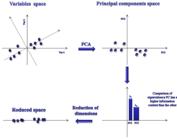
Assuming to have a data set consisting of n objects, each of them described by p variables, a data exploration can be performed to detect some information about statistical parameters relative to each variable, the correlations between the variables, and the presence of outliers. In particular, the principal component analysis (PCA) is one of the best methods for data exploration in multivariate systems.

Discrimination deals with the separation of groups of data while classification requires a

priori class description. In this case the aim of the data analysis is to assign, to classify, new

objects to the defined classes. Here also PCA can be used but in the experimental problem here faced the most useful chemometric classification approach is the Soft Independent Modeling of Class Analogy (SIMCA).

The methods of regression calculate mathematical models allowing to predict quantitative values of a variable (response) from the values known for n samples and taken from a set of independent variables (predictors). If it is considered that the model can assume a character of general validity, it becomes independent from the specific set of data used. The most used regression methods are: Principal Component Regression (PCR) and the Partial Least Square Regression (PLS-R).

26

A2-2 Multivariate structure data

Chemometric techniques normally apply to data structures represented by a table of numbers (data matrix) consisting of a number of observations, each of which is represented by

variables that describe the observations (Figure A2-2). The data matrix is indicated with the

symbol X and represented in this form:

The n rows of X are objects and can be samples, experiments. The p columns of X are the variables and can be: properties. An element of X is written_, with i = 1, .... n and j = 1, ..., p.

The variables or descriptors are the quantities used to study a given phenomenon and to describe the overall experimental observations and can be measured or calculated. The variables may be: independent variables or predictors and dependent variables or responses. It is essential to highlight the possible existence of variables that, although having different meanings, carry the same information or have the same ability to quantitatively represent the system under study. To highlight the roles of variables, we rewrite the matrix data in the form ( Figure A2-3):

Figure A2-2 Data matrix

27

The objects are examples or samples available to understand the studied phenomenon, to construct mathematical models, to confirm the assumptions made.

An object can be described in full if, for all the variables selected to describe it, there are values that apply to it. In other cases, as frequently happens, no data are available for all variables selected and the object description is incomplete: it is said that there are missing

values .

A2-3

Data pretreatment

Before performing any kind of processing a preliminary analysis of the data is always necessary, aiming to control and prepare the data for subsequent processing. In checking data, it is suggested to ensure absence of transcription errors, occurrence of missing data and choice of correct orders of magnitude.

The fundamental pretreatments are: transformation of variables, data scaling, and

replacement of missing data.

A preliminary check on the variables consists of the following tests: • there not should be constant variables: they would have no variance

• there not should be degenerate variables: they vary little with changes of objects and give variance tending to zero

• there not should be discrete variables: they require a particular statistical We proceed to the transformation of variables to control abnormalities such as: • lack of linearity

• lack of normality • lack of additivity

• the variables have variances of very different orders of magnitude • the system is not very strong

28 Table A2-I

LOGARITHMIC TRANSFORMATION log1

POWER TRANSFORMATION !

INVERSE TRANSFORMATION "

SQUARE ROOT TRANSFORMATION #.$

When searching for information about relationships between variables, it is important to maximize the comparability between the variables. A difference of several orders of magnitude on average values result in several orders of magnitude of difference on the variances and therefore a statistical comparison is not possible. In these cases it is appropriate to apply a data scaling data can be performed in different ways. The most common are:

• Centering (CS) • Maximum scaling (MS) • Range scaling (RS) • Autoscaling (AS) Table A2-II CENTERING,CS % '& MAXIMUM SCALING,MS /) RANGE SCALING,RS % */)% * AUTOSCALING,AS % '/+&

Uj = maximum value j-th column; Lj =minimum value j-th column; sj = standard deviation

In many cases it happens that no samples are available for all the values for all variables that describe them. This unpleasant aspect of the data forces us to take some decisions, because none of the common mathematical methods can deal with problems where some values are missing in the data matrix. To solve this problem there are several possibilities:

29

• Removal of samples

The simplest method uses the removal of samples for which there is data missing. This is a good solution only if the number of samples is high and therefore the elimination of some sample does not entail the loss of relevant information.

• Elimination of variables

An alternative to the previous case is the elimination of one or more variables for which there are a number of missing data, and then retaining only those variables for which all values are available.

• Substitution with the average

If missing data are not too many, the missing value can be replaced with the mean value calculated over all the remaining data relevant to the involved variable.

• Replacement by a random value

The missing data are replaced by a random number such as -999. • Replacing using regression

The missing values for each variable are predicted using a regression model derived from all samples with no missing values.

• Replacing using local similarity

This method for the calculation of missing values is based on the method of classification K-NN (k-nearest neighbors).

• Replacing using the principal component analysis

The principal component analysis is performed using all the known values and applying an algorithm that allows to calculate the main components even with incomplete matrices.

30

A2-4 Principal component analysis

A2-4.1 Introduction

The principal component analysis (PCA) is one of the fundamental techniques for multivariate analysis. It was introduced by Karl Pearson in 1901 and developed in its present form in 1933 by Harold Hotelling. It is the most important exploration data technique and it consists in transforming the original variables into new variables, called principal components (or latent variables), obtained by linear combination of the original variables and orthogonal to each other.

The PCA allows to:

• evaluate correlations between variables and their relevance • display objects (identification of outliers, classes, etc.)

• summarize the data description (removal of noise or spurious information)

• reduce the data dimensionality

• individuate major properties

• develop a model of data representation in an orthogonal space

A2-4.2 The principal components

The calculation of the principal components is divided into several steps that lead to a matrix ,, matrix of eigenvectors,

,- λ- A2-1

where λ is an eigenvalue and is related to the explained variance.

The first step consists in the calculation of the correlation matrix C ( p x p ), defined as:

/,0

1 _/,0

n-1 A2-2

where:

• X is the data matrix ( n x p )

•

45

6786:::9

;8

'

∑=7>?678

31

+

A

=

7>? B

@"

The correlation matrix compares variables with each other; the term C quantifies the correlation between variables i and j:

• C D 0 means there is a positive relationship between the variables

• C F 0 means there is a negative relationship between the variables

• C 0 means there is no correlation

The diagonalization of the correlation matrix C results in the eigenvalues matrix G ( p x p) whose diagonal elements are the eigenvalues H_I (m= 1,….,p):

G JKLM A2-3

By the process called Single Value Decomposition (SVD) which is based on the following equation:

, G ,1 A2-4

the matrix of the eigenvectors A is determined:

A = N O O O PQ_{R R}"" R Q_R"I R Q_{R R}"S Q" R QI R QS R R R R R Q_S" R Q_SI R Q_SSTU U U V HI

The equation A2-4 corresponds to the operation of rotation that defines a new space, called

eigenspace, whose axes, the eigenvectors, are oriented in the direction of maximum variance,

in descending order. Each eigenvalue is proportional to the variance associated with the corresponding principal component and the sum of all the eigenvalues is equal to the total

32

variance of the data. Considering the matrix A and assuming that the smallest eigenvalues are associated with not relevant information, the eigenvalues are examined and the first M largest eigenvalues retained. The matrix obtained with the first M eigenvectors is denoted by L (p x

M) and is called the loadings matrix, whose columns represent the PC and whose rows

represent original variables.

Loadings are standardized linear coefficients, i.e. the sum of squares of the loadings of an eigenvector is equal to 1, or the eigenvectors have unit variance; consequently the relations:

%1 W Q_I W 1 ∑ Q _IX 1 A2-5 A value of ljm close to 1, in absolute value, indicates that the m-th component is represented

mostly by the j-th original variable; vice versa, a value of ljm close to zero indicates that the

j-th variable is not represented in j-the m-j-th component.

Multiplying together the data matrix X and the loadings matrix L , a new matrix T called

scores matrix is determined :

1 /Y A2-6

Scores values are the result of a linear combination, in which the variables are the original variables (usually scaled) and the coefficients are the loadings of the m-th component:

ZI ∑ [I A2-7

Thus:

ZI \]. [I A2-8

where xT and l are p-dimensional vectors being p the number of original variables. Unlike loadings, scores have mean value equal to zero, but can take any numerical values. The scores represent the new coordinates of the objects in the space of principal components.

Applying the inverse formula:

^_ 1Y1 _A2-9

the data reproduced matrix is obtained: if the number of principal components is less than the original variables, the new matrix is an approximation of the original one, as spurious information ( i.e. the noise ) has been eliminated.

33

A2-4.3 Loading and score plots

In each multivariate analysis is important to display the results obtained by simple and intuitive plots allowing an immediate graphical interpretation.

PCA provides an algebraic solution that determines very effective graphical representations both of objects (score plot) and of variables (loading plot).

The loading plot allows analyzing the role of each variable in the different components, their direct and inverse correlations, and their importance (Figure A2-4).

Consider the simplest case and choose only two principal components, PC1 and PC2, which are the two columns of the matrix of loadings L (p x 2). This matrix has m rows, which correspond to the original variables or to the columns of the data matrix X. The elements of L vary between -1 and 1. Each variable is characterized by a pair of loadings, lj1 and lj2:

• lj1 quantifies the relevance component of the variable xj in PC1

• lj2 quantifies the relevance of the variable xj in component PC2.

The loading plot is constructed by representing, in the plane lj2 vs. lj1, the points

corresponding to the p original variables. The interpretation of the loading plot is based on some fundamental observations.

• Points near the origin correspond to variables not relevant to any principal components choices.

• Points on the horizontal axis correspond to variables that are irrelevant for PC2. • Points on the ordinate correspond to variables that are irrelevant for PC1. • Points with abscissa of absolute values are very important for high PC1.

34

• Points ordered with high absolute value are very important for PC2.

• Points close to each other correspond to variables that carry similar information. • Points symmetrical to the origin correspond to varying inversely related.

The score plot shows the behavior of the objects in the different components and their similarity (Figure A2-5).

As in the previous example, only two principal components PC1 and PC2, which are the first two columns of the matrix of loadings L, have to be considered. The product of X and L gives the matrix T (n x 2). This matrix has n rows, which correspond to objects or to the rows of the data matrix X. Each object is characterized by a pair of scores, tj1 and tj2 that are the

coordinates in the space of the components PC1 and PC2. The most commonly used plot in

multivariate analysis is the score vector for PC2 versus the score vector PC1. This is to due to the fact that these are the two directions of largest and second largest variances.

The score plot is constructed in the plane tj2 vs. tj1 reporting the n points corresponding to the n objects of the problem. There are two rules of thumb concerning score plots:

• Always use the same couple of principal component in all score plots: this will help getting the desired overview of the compound structure data.

• Choose as ordinate the principal component that has the largest “problem relevant” variance. For many applications this will turn out to be PC2, but it is possible that, in other cases, PC2 lies along a direction that for some problem-specific is not interesting.

35

The score plot represents the objects in the space of components principal and is very effective to search for outliers and clusters graphically. The comparison of score plots and loading plots allows determining which variables are relevant to the n objects. There is a "quadrants" correspondence between the two graphs (Figure A2-6):

A2-4.4 Geometric interpretation of PCA

Geometrically, the PCA appears as a rotation from the original space to the space of principal components; this process is performed in such a way that the first new axis, i.e. the first

principal component, PC1, is oriented in the direction of maximum variance data and all the

next axes are orthogonal to each other.

Consider for simplicity the case of a two-dimensional system; the variables space will have 2 axes: var1 and var2. Each object is represented by a set of variable measurement and characterized by its coordinate (x1, x2)in the Cartesian coordinate system (Figure A2-7).

36

Each object can be plotted as a point, and the result is a swarm of points showing a trend of the objects to arrange in a particular direction. A central axis could be drawn through the swarm: this line would describe the data almost as efficiently as all the original variables. This central axis is positioned along the direction of maximum variance and is called first Principal

Component or PC1. The second principal component will lie along a direction orthogonal to

first PC and in the direction of the second largest variance.

One of the purposes of PCA is to reduce the dimensionality of a multivariable system: a transformation from two dimensions to only one may seem trivial but it allows to understand the true meaning of this method of exploration. If it is assumed to be able to represent the points with the only new coordinate PC1 is right to assess the extent of this approximation. This means verifying how much information is lost. In Figure A2-7 a comparison between the eigenvalues associated to the principal components PC1 and PC2 is reported.

It’s evident that λ1> λ2 and since the variance (and therefore the information) is related to

this parameter, a dimensions reduction performed by a projection of the objects on the axis PC1 does not cause a significant loss of information.

37

The example illustrated above can easily be generalized to a p-dimensional system, determining the principal components PC1, PC2, PC3 etc. The first principal component contains the highest percentage of variance, the second a smaller percentage and so on, until the last components bring with them a negligible amount of variance.

A2-4.5

One of the fundamental problems that the principal component analysis presents is the determination of the significant number M of components (factors), with M < p. The search for the number of significant components is known as rank analysis. In fact, if data contains an information structure (i.e., non random), separation between the variability due to experimental noise or spurious information and the useful information is achieved through a proper definition of the number of significant principal components. Any selection procedure of a reduced number of significant components assumes that the variability of useful information is greater than the variability associated with the experimental noise or secondary information.

Generally two methods, a numerical and a graphic one, are used.

The numerical method is based on the concept of percentage explained variance by M

principal components, which represents an estimate of the importance of information derived from a certain principal component. Since each eigenvalue represents the variance associated with the corresponding principal component and the sum of all the eigenvalues coincides with the total variance, the percentage explained variance for the m component compared to the total variance is given by:

`aI% ∑dc>?!c!c e 100 A2-10

The cumulative explained variance relative to the first M principal components is given by:

fgh_{. `ai%} ∑jc>?!c

∑dc>?!c e 100 A2-11

38

kai% ∑ !c

d c>jl?

∑dc>?!c e 100 A2-12

The right number of PCs would be the one corresponding to a cumulative variance greater than a given threshold value; a common choice of thumb is to consider as a threshold the 80% of the total variance. What is important is to minimize the value of RV to be sure not to lose too much information.

The number of principal components to be considered can be determined by the analysis of the eigenvalues graphics plotted against the number of factors. In this type of graph, known as

scree plot, the number of components is reported on the abscissa and on the ordinate axis the

corresponding eigenvalues (Figure A2-8).

It’s evident that the first principal components are associated with a greater percentage of explained variance, while the subsequent PCs are associated with a smaller amount of information (asymptotic behavior). A proper criterion of choice is to maintain only the first n PC for which a profound change in the slope of plotted line is manifested.

39

A2-5 SIMCA (Soft Independent Modeling of Class Analogy)

Classification is one of the fundamental aims of multivariate data analysis:

• To identify and quantitatively characterize subgroups within a given set of samples.

• To assess whether a new sample is similar to other samples, or to which group it belongs,

• To identify samples that are dissimilar compared to some standard

The Soft Independent Modeling of Class Analogy (SIMCA) represents one of most used chemometric classification approach based on similarities and is able to determine whether one or more new samples belong to an already existing group of similar samples.

The basis of this classical chemometric technique (Wold, 1976) is that objects in one class, or group, show similar rather than identical behavior and new objects are assigned to the class to which they show the largest similarity.

The SIMCA classification distinguishes two cases:

• Classes are known a priori i.e. the specific belonging of all the training set objects is known

• There is no a priori class membership available

The SIMCA approach presents some powerful advantages compared to methods like e.g. Linear Discriminant Analysis (LDA). Firstly SIMCA does not require that the number of objects is significantly larger than the number of variables as is invariably the case with classical statistical techniques: the present bilinear methods are effective regardless of the value of the ratio objects/ variables, be it either (very) many objects with respect to variables - or vice versa.

A further reason that makes SIMCA a powerful tool for classification regards the possibility of graphically representing the results with a great insight relatively to the specific data structures behind the modeled patterns.

In the classification of a new set of data, SIMCA calculates extensive statistics that enable to quantify “model envelopes”, or classification spaces, surrounding the classes. By defining the distance between the envelope and the model, it can be geometrically assessed whether new samples lie inside or outside a given model. It is thus possible to establish the model distances almost entirely by graphical means, although the full numerical result complement is of course also available in the background

40

Many plots are available to interpret the object/class-model relationships such as the well-known Coomans plot that gives the information about the class membership to any two

models simultaneously. The Unscrambler® is the software here applied for this kind of data

analysis.

A2-5.1

SIMCA can be defined as a multi-application use of PCA-modeling as classification model; it usually consists of several PC-models, one for each class recognized. The first step is always a class modeling, i.e. to group the different object into homogeneous classes or clusters. Then each class is centered, scaled and modeled separately. Finally the new objects can be allocated to the established classes - or they may fall outside all “known” patterns.

In detail, the various steps of method are reported:

1. A data pretreatment is suggested.

2. A projection model of all objects to start to identify the individual classes is performed.

3. The pattern-specific classes and the discrimination between classes are simultaneously

defined. All the relevant score plots have to be studied and all the problem specific groups or clusters identified. It has to be determined which objects belong to each subgroup in this training stage. There is always a great deal of interaction between the general problem context and the initial data analysis results in this stage.

4. A separate model for each class is delineated and all classes must be validated in the exact same way, or the membership limits will not be comparable.

5. It’s necessary to remove outliers and to study the appropriate score plots to see if there should be more classes present than what is “known" in advance .

41

At this stage, the new data set can be classified; the data must of course be described by the

same set of variables as for the training class models. If the calibration data (used for creating

the class models) were in some way transformed, the new data must also be transformed in exactly the same way before classification. After choosing the class models to be used for the

pattern recognition, the number of PCs to use in each model has to be defined (this is strongly

problem-depend). The appropriate number of PCs depends on the data set, the goal, and the application.

Classifying a new object can result in several different results:

1. The object is uniquely allocated to one class, i.e. it fits to a single model within the given limits and is very far from the other classes.

2. The object may fit several classes, i.e. it has a distance that is within the critical limits of several classes simultaneously. This behavior can depend on either the given data are insufficient to distinguish between the different classes or the object actually does belong to several classes. It may be a borderline case or have properties of several classes.

3. The object fits none of the classes within the given limits. This is a very important result in spite of its apparent negative character. This may mean that the object is of a

new type, i.e. it belongs to a class that was unknown before or - at least - to a class that

has not been used in the classification. Alternatively it may simply be an outlier.

An important and peculiar aspect which makes SIMCA a powerful tool for the classification is to consider “failed” pattern recognition as an option of classification output. Clearly it is important to be able to identify such potentially important “new objects” with some measure of objectivity. It is therefore important to be able to specify the level of statistical significance associated with SIMCA results.

42

A2-5.2 Statistical Significance Level in SIMCA

Statistical significance tests are based on the concern of making mistakes. In the setup used in SIMCA-classification, the test quantifies the risk of saying that a particular object lies

outside a specific model envelope. In The Unscrambler® classification results can be studied

with varying significance levels - usually between 0.1% and 25% - whose value is chosen depending on the particular problem.

The “normal” statistical significance level used is 5%. i.e. there will be a 5% risk that a particular object falls outside the class, even if it truly belongs to it; 95% of the object which truly belong will thus fall inside the class. At opposite ends of the significance levels typically used it is noted that:

• Choosing a high significance level (e.g. 25%) means that only very “certain” objects will belong to the class, and (many) more “doubtful’ outside it. Fewer objects that truly belong will fall inside the class (in this case,75%).

• Choosing a low significance level (e.g. 1%) means that cases, which are doubtful, will still be classified as be belonging to the class. More objects will be classified as members, i.e. almost all of the true member objects (i.e. 99%) will be members of the class.

A2-5.3 The Coomans Plot

This plot shows the orthogonal (transverse) distances from all new objects to two selected models (classes) at the same time. The critical, cut-off class membership limits are also indicated. These limits may be changed by editing the significance level.

43

The two straight lines divide the space into four quadrants; the position of the straight lines is linked to the chosen significance level (Figure A2-9). The objects are assigned in this way:

1. In the first of the four quadrants the objects assigned to none of the selected models are placed

2. The zone 2 contains objects assigned to model B

3. In the zone 3 the objects assigned to both methods are placed 4. The objects placed in the last quadrant are assigned to model A

To make interpretation easier, the objects are color coded in The Unscrambler® ( Figure A2-10).

44

45

CHAPTER

B1

BEHAVIOUR OF

PHOSPHOLIPIDS IN

ANALYTICAL REACTIVE

PYROLYSIS

*

*Manuscript of the following article:

46

B1-1 Keywords

Gas chromatography-mass spectrometry Pyrolysis Derivatisation Phospholipids Tempera Pigments B1-2 Summary

Checking for the presence of egg in a painting layer allows to decide whether or not it is a tempera.

Several already assessed analytical techniques may be used to perform the chemical analysis for the detection of egg in paintings.

As an advantageous, alternative methodology for the determination of egg, a new application of analytical pyrolysis, hyphenated with gas chromatography-mass spectrometry (GC-MS) system, in presence of hexamethyldisilazane (HMDS) and tetramethylammonium hydroxide (TMAH), is here reported. The innovation lays mainly in the choice of new markers for the presence of egg. It is here demonstrated that in art diagnostic Tris-TMS-ester and methyl-ester of phosphoric acid, generated by the pyrolysis of standards phospholipids and synthetic painting layers containing egg as binding medium, may be used as new markers for identification of egg in tempera layers. The adoption of these new markers in analytical pyrolysis allows to obtain higher analytical performance with respect to classical markers (fatty acids), especially in terms of yield and, as a consequence, in terms of limit of detection.

B1-3 Introduction

Egg is a very complex matrix consisting of two separated phases: egg-white and egg-yolk. Egg-white is an aqueous colloidal solution of proteins, mainly albumins, and low quantities of fats, while egg-yolk can be considered as an emulsion, that is a colloidal dispersion of phosphorated proteins and lipids. The lipidic fraction is the most consistent in egg-yolk, and is made up of triglycerides (65%w/w), phospholipids (29% w/w) and cholesterol (5.2% w/w) [12-13]. The phospholipids are triglycerides in which a phosphoric group esterifies one hydroxyl group of glycerol. This gives rise to a mono-glyceride of the tribasic phosphoric