ISSN: 2088-8708 2239
Sliding-Mode Controller Based on Fractional Order Calculus
For a Class of Nonlinear Systems
Noureddine Bouarroudj*, Djamel Boukhetala*, and Fares Boudjema*
*LCP, Ecole Nationale Polytechnique, 10 av. Hassen Badi, BP. 182, El-Harrach, Alger, Algeria
Article Info Article history: Received Apr 12, 2016 Revised July 18, 2016 Accepted Aug 7, 2016 Keyword:
fractional order culculus SMC
FOSMC
inverted pendulum
ABSTRACT
This paper presents a new approach of fractional order sliding mode controllers (FOSMC) for a class of nonlinear systems which have a single input and two outputs (SITO). Firstly, two fractional order sliding surfacesS1andS2were proposed with an intermediate variable z transferred fromS2 to S1 in order to hierarchy the two sliding surfaces. Secondly, a control law was determined in order to control the two outputs. A sliding control stability condition was obtained by using the properties of the fractional order calculus. Finally, the effectiveness and robustness of the proposed approach were demonstrated by comparing its performance with the one of the conventional sliding mode controller (SMC), which is based on integer order derivatives. Simulation results were provided for the case of controlling an inverted pendulum system.
Copyrightc 2016 Institute of Advanced Engineering and Science. All rights reserved. Corresponding Author:
Noureddine Bouarroudj
LCP, Ecole Nationale Polytechnique, 10 av. Hassen Badi, BP. 182, El-Harrach, Alger, Algeria Email: [email protected]
1. INTRODUCTION
Sliding mode control has largely proved its effectiveness in numerous applications, see, e.g., the studies by Utkin [1] and Slotine [2]. The first step of the SMC design is to select a sliding surface that models the desired closed-loop performance in state variable space. In the second step, equivalent and hitting control laws are designed such that the system state trajectories are forced towards the sliding surface and slide along it to the desired attitude.
An advantage of these methods of control (SMC) is their robustness to parameters variation and bounded external disturbances. The robustness is attributed to the discontinuous term in the control input. However, this discontinuous term also causes an undesirable effect called chattering. Sometimes this discontinuous control action can even cause instability of the system. This effect can be alleviated by, for example, introducing a sat function and taking off the sgn function in the hitting control law of the SMC.
In the last years, the control of single-input-two output non-linear dynamical systems has risen some interest in the control research community; in general, the controller (input) is done for the trajectory tracking of the two out-puts. PID controllers were applied in [3] to the stabilization and tracking control of three types of inverted pendulum. A PID+LQR method was given in [4], in which the LQR was added negatively to the PID in order to have a resultant optimal control. A fuzzy controller with estimation of scaling factors was studied in [5]. An intelligent control system based on an interval type-2 fuzzy PD controller was studied in [6]. The SMC design for this kind of systems is a very challenging task. Such developed controllers include the decoupled SMC shown in [7], a Fuzzy Sliding Mode Con-trol (FSMC) that was tuned using ant colony optimization [8], [9] and a decoupled SM with a fuzzy-neural network controller [10] where the fuzzy-neural network was used to approximate an ideal computational controller. All these developed approaches are based on the standard integer order calculus.
The fractional order differentiation theory, which has 300 years of history and deals with derivatives and integrals of non-integer order, has recently been rediscovered by scientists and engineering, being applied in many fields and, among them, the field of control. One of the first applications of fractional order derivatives/integrals to the control of dynamic systems was given by Oustaloup, who developed the so called Commande Robuste dOrdre Non Entier (CRONE) ,which is described in [11, 12], along with examples of application in various fields. Fractional order
PID (FOPID) controllers have been studied in [13]. A fuzzy FOPID controller, which uses the error and its fractional order derivative as its input, and has a fractional order integrator in its output, has been proposed in [14].
Also in the SMC field, some researchers have introduced the fractional order calculus to design a fractional order sliding mode control (FOSMC). The first application using the technique of fractional order SMC returns to Calderon [15, 16] on a DC-DC power converter; where the authors defined switching surfaces based on the structures of fractional order PI (FOPI) and FOPID controllers. The approach which uses the FOPID sliding surface was also studied in [17, 18]. A FOSMC based on a fractional order PD (FOPD) sliding surface was studied in [19, 20] and a Fractional Order Terminal Sliding Mode Control (FOTSMC) was proposed in [21].
Motivated by the above discussion, this paper proposes a FOSMC for a class of single input two outputs non-linear systems. The control law is derived from these proposed fractional order sliding surfaces and its purpose is to drive the two outputs of the system to their desired trajectories. The stability is guaranteed by using the Lyapunov theorem. Simulation results illustrate that the proposed control design method applied to the inverted pendulum plant yield controller that can rapidly stabilize these system compared with the conventional integer order controller. This performance is guaranteed through the added extra parameterα(fractional order).
The rest of this article is organized as follows. A brief introduction to fractional calculus is described in Section 2. System description and control design are developed in Section 3. Simulation results and some conclusions are given in Sections 4 and 5 respectively.
2. A BRIEF INTRODUCTION TO FRACTIONAL CALCULUS
The fractional differo-integral operators are denoted byaDtαf(t)(fractional calculus), whereaandt, are the
bounds of the operation andα∈ Ris a generalization of the standard integration and differentiation to non-integer order operators.
The continuous differo-integral operator is given by the following:
aDαt = dα dtα f or α0 1 f or α= 0 Rt a(dτ) α f or α≺0 (1)
In the literature We can find different definitions of the fractional differ-integral operator. But the most commonly used definitions of fractional order derivatives are:
The Riemann-Liouville (RL) definition:
aDαtf(t) = 1 Γ(m−α) d dt mZ t a f(τ) (t−τ)1−(m−α)dτ (2)
The Caputos definition:
aDαtf(t) = 1 Γ(m−α) Z t a fm(τ) (t−τ)1−(m−α) dτ (3)
In these expressions,m−1< α < m, andΓ(.)is the well-known Eulers gamma function:
Γ(x) = Z ∞
0
e−tt(x−1)dt, x >0 (4)
On the other hand, Grunwald-Letnikov (GL) reformulated the definition of the fractional order differ-integral operator as follows: aDtαf(t) = lim h→0 1 hα (t−a)/h X k=0 (−1)k α k f(t−kh) (5)
Since the numerical simulation of a fractional differential equation is not as simple as an ordinary differential equation, the Laplace transform method is often used as a tool for solving fractional order differential equations that arise in engineering applications [22], [23].
The Laplace transform of the (RL) definition is as follows [22], [24]: L{0Dαtf(t);s}=s αF(s) − (m−1) X k=0 skh0D (α−k−1) t f(t) i t=0 (6)
The Laplace transform of the Caputos definition is given by [24]:
L{0Dαtf(t);s}=sαF(s)−
(m−1) X
k=0
s(α−k−1)fk(0) (7)
Wheresdenotes the Laplace operator. For zero initial conditions, the Laplace transforms of the fractional order derivatives of Riemann-Liouville and Caputo are reduced to (8) [24], [25].
L(0Dαtf(t)) =sαF(s) (8)
In this paper, the fractional order elementsαis approximated by the Oustaloups filter. The Oustaloups filter
[26] approximates
G(s) =sα, α∈R (9)
by a rational function of the form
ˆ G(s) =K N Y k=−N s+w0k s+wk (10)
where its parameters (zeros, poles, and gain) are determined by the following formulas:
wk0 =wb. wh/ wb (k+N+0.5(1−α))/(2N+1) wk =wb. wh/ wb (k+N+0.5(1+α))/(2N+1) K=wαh (11)
In these expressions, (2N+ 1) is the order of the filter and wb and wh are respectively the low and high transient-frequencies.
In the following, some properties of the Caputos definition of fractional order derivatives that will be used in this paper are given. The below desirable properties are valid under causality and when the function is differ-integrated taking as starting point the point when the function starts [24]:
- Fractional order derivative of the fractional order integration of the functionf(t):
aDαt(aDt−αf(t)) =f(t) (12)
- Fractional order integration of the fractional order derivative of the functionf(t):
aDt−α(aDtαf(t)) =f(t)− m−1 X k=0 fk(a) k! (t−a) k (13)
- The fractional order derivative is a linear operator:
aDαt(f(t) +g(t))=aDtαf(t)+aDtαg(t) (14)
- The fractional order integration is a linear operator:
3. SYSTEM DESCRIPTION AND CONTROL DESIGN 3.1. System description
Consider the single-input two-output non-linear system, which can be represented in the following state space form: ˙ x1=x2 ˙ x2=f1(x) +b1(x)u+d1(t) ˙ x3=x4 ˙ x4=f2(x) +b2(x)u+d2(t) (16)
WhereX = [x1, x2, x3, x4]T is the state vector,f1(x),f2(x)andb1(x),b2(x)are nonlinear functions, u is the control input,d1(t),d2(t)are bounded external disturbances. Moreover assume thaty = [x1, x3]T is the output vector.
Assumption 1: The bounded external disturbances satisfy the following inequalities:
|d1(t)| ≤δ1 (17) |d2(t)| ≤δ2 (18) D (α−1) t d1(t) ≤ψ1 (19) D (α−1) t d2(t) ≤ψ2 (20)
Whereδ1,δ2,ψ1andψ2are known positive constants.
3.2. Sliding Mode Controller (SMC) Design
The principle of the proposed methodology to design the SMC for system (16) is the following:
- Decouple the global system into two subsystems. The first one contains the statesx1,x2, and a sliding surfaceS1 = ˙e1+λ.e1is defined for it, wheree1 =x1−x1dandλ1is a positive constant. The second subsystem contains the statesx3,x4, and a sliding surfaceS2 = ˙e3+λ.e3is also defined for it, wheree3 =x3−x3dandλ2 is another positive constant. Note that the control objective is to force a motion of the states of the first subsystem towards the sliding surfaceS1 = 0, converging therefore tox1=x1d,x2 = ˙x1d. The second objective is to force a
motion of the states of the second subsystem towards the sliding surfaceS2 = 0, converging therefore tox3 =x3d,
x4= ˙x3d.
- The use of a control signalu=u1calculated from the sliding surfaceS1 causes the convergence of only the statesx1,x2to their desired values. And the use of a control signalu=u2calculated from the sliding surfaceS2 causes the convergence of only the statesx3,x4to their desired values. In order to achieve simultaneous control of all the states, we take into account the idea of [8] that consists in using an intermediate variablezbetween the sliding surfaces. This variable represents the information transferred fromS2toS1, and saturates the errore1tok2. Thus the sliding surfaceS1is modified to
S1= ˙e1+λ1.(e1−z) (21)
While the sliding surfaceS2keeps its standard form
S2= ˙e3+λ2.e3 (22)
- This modification changes the control objective from makingX =Xd = [x1d, x2d, x3d, x4d]T to making
X = ˆXd= [x1d+z, x2d, x3d, x4d]T where
z=.sat(S2/φ2).k2, 0< k2<1 (23)
And the definition of thesat(.)function is: sat(S2/φ2) =
(S2/φ2) if |S2/φ2|<1 sgn(S2/φ2) if |S2/φ2| ≥1
(24) Beingφ2is the boundary layer of the sliding surfaceS2.
Remark: IfS1 = 0, then we obtain from equation (21) thatx1 = x1d+z andx2 = ˙x1d. On the other
decreases the value ofS2, which implies that the value ofzdecreases too. In such case, ifz→0andS1→0too, we would have thatx1 → x1d. In summary, we can state that whenS2 →0andS1 → 0, thenx3 → x3d,z →0and
x1→x1d, and the control objectives would be achieved.
Keeping the system states (x1, x3) on the sliding surfacesS1,S2,∀t >0guarantees that the tracking errors vector (e1,e3) asymptotically approaches to zero. The corresponding sliding condition is [10]:
V = 12S2 1 ≥0 ˙ V =S1S˙1 ≤0 (25) The general control structure that satisfies the stability condition of the sliding motion can be written as:
u=ueq+usw (26)
Whereueq is called the equivalent control law that is derived by settingS˙1 = 0andusw is the switching
control law.
Taking the time derivative of (21) gives: ˙
S1= ¨e1+λ1.( ˙e1−z˙) = (¨x1−x¨1d) +λ1.( ˙e1−z˙)
= (f1(x) +b1(x)u+d1−x¨1d) +λ1.( ˙e1−z˙)
(27) Where,z˙is given as follows:
˙ z= k2 φ2. ˙ S2 if S2 φ2 ≺1 0 if S2 φ2 ≥1 (28) And: ˙ S2= ¨e3+λ2.e˙3 = (¨x3−x¨3d) +λ2.e˙3 = (f2(x) +b2(x)u+d2−x¨3d) +λ2.e˙3 (29)
Substituting equations (29), and (28) into (27), and settingS˙1= 0in this last equation, the equivalent control is obtained: ueq = −1 (b1−λ1kφ22b2) [f1−x¨1d−λ1 k2 φ2 .(f2−x¨3d) + (λ1.e˙1−λ1λ2 k2 φ2 .e˙3)] (30)
Then the global control inputuis given by the expression:
u= −1 (b1−λ1kφ2 2b2) [f1−x¨1d−λ1 k2 φ2 .(f2−x¨3d) + (λ1e˙1−λ1λ2 k2 φ2 .e˙3) + (k1.sgn( S1 φ1 ))] (31)
wherek1is a positive constant andφ1is the boundary layer of the sliding surfaceS1. Substituting (31) into (27) yields ˙ S1= d1−λ1φk22.d2 −k1sgn(Sφ11) ≤δ1.sgn(Sφ1 1)−λ1 k2 φ2.δ2.sgn( S1 φ1) −k1.sgn(Sφ1 1) (32) Then simply: S1S˙1≤φ1. δ1−λ1 k2 φ2 .δ2−k1 . S1 φ1 (33) From Eq(33) it can be concluded that the reaching condition is obtained fromk1(δ1−λ1φk2
2.δ2).
But, Eq(31) will have high-frequency switching near the sliding surface (S1 = 0) due to the sgn function involved. Thus, in order to reduce the chattering phenomenon, we replacesgn(S1/φ1)bysat(S1/φ1)as follows:
u= −1 (b1−λ1φk2 2b2) [f1−x¨1d−λ1 k2 φ2 .(f2−x¨3d) + (λ1.e˙1−λ1λ2 k2 φ2 .e˙3) + (k1.sat( S1 φ1 ))] (34)
3.3. Fractional Order Sliding Mode Controller (FOSMC) Design
In this section we will develop a fractional-order sliding mode control for trajectory tracking of the system of Eq(16). For this purpose, the forms introduced in the previous section are used.
Let the two sliding surfaces to be defined as follows:
S1=Dtαe1+λ1.(e1−z) (35)
S2=Dαte3+λ2.e3 (36)
With respect the property of Caputos derivativeDα
t(f(t)) =D
(α−m)
t
dm
dtm(f(t)),S1andS2can be rewritten as : S1=D (α−1) t e˙1+λ1.(e1−z) (37) S2=D (α−1) t e˙3+λ2.e3 (38)
Taking derivative of both sides of Eq(37) with respect to time, we have. ˙ S1=D (α−1) t ¨e1+λ1.( ˙e1−z˙) =D(tα−1)(¨x1−x¨1d) +λ1.( ˙e1−z˙) =D(tα−1)(f1(x) +b1(x)u+d1−x¨1d) +λ1.( ˙e1−z˙) (39)
Where,z˙has the same form as in Eq(28), and: ˙ S2=D (α−1) t e¨3+λ2.e˙3 =D(tα−1)(¨x3−¨x3d) +λ2.e˙3 =D(tα−1)(f2(x) +b2(x)u+d2−x¨3d) +λ2.e˙3 (40)
By settingS˙1= 0and respect the properties of fractional derivative given in section II; the equivalent control is obtained and it has the flowing formula:
ueq= −1 (b1−λ1φk2 2b2) [f1−x¨1d−λ1 k2 φ2 .(f2−¨x3d) +D (1−α) t (λ1.e˙1−λ1λ2 k2 φ2 .e˙3)] (41)
Then the global control inputuis given by:
u= −1 (b1−λ1φk22b2) [f1−x¨1d−λ1 k2 φ2 .(f2−x¨3d) +D (1−α) t (λ1e˙1−λ1λ2 k2 φ2 .e˙3) +Dt(1−α)(k1.sgn( S1 φ1 ))] (42)
Whereuswis given by its proper formula in Eq(42) to satisfy the existence condition of sliding mode. For
the stability condition, substituting Eq(42) into Eq(39); results in:
˙ S1=−D (α−1) t D (1−α) t (λ1.e˙1−λ1λ2φk2 2.e˙3)−D (α−1) t D (1−α) t (k1.sgn(Sφ1 1)) + (λ1.e˙1−λ1λ2 k2 φ2.e˙3) +Dt(α−1)d1−λ1kφ2 2.D (α−1) t d2 (43)
Taking into account the property of Caputos derivativeaD−αt (aDtαf(t)) =f(t)−
m−1 P k=0 fk(a) k! (t−a) k, where m= 1.
This lets us have:
˙ S1=−k1.(sgn( S1 φ1 )) +k1.(sgn( S1(0) φ1 )) + (λ1.e˙1(0)−λ1λ2 k2 φ2 .e˙3(0)) +D (α−1) t d1−λ1 k2 φ2 .D(tα−1)d2 (44)
If one assume thatk1.(sgn(S1φ(0)
1 )) + (λ1e˙1(0)−λ1λ2
k2
˙ S1=−k1(sgn(Sφ1 1)) +D (α−1) t d1−λ1kφ2 2.D (α−1) t d2 =−k1(sgn(S1 φ1)) +ψ1(sgn( S1 φ1))−λ1 k2 φ2.ψ2(sgn( S1 φ1)) (45) Then simply: S1S˙1≤φ1. ψ1−λ1 k2 φ2 .ψ2−k1 . S1 φ1 (46) From Eq(46) the reaching condition can be obtained fromk1(ψ1−λ1φk2
2.ψ2). Otherwise, if k1.(sgn( S1(0) φ1 )) + (λ1e˙1(0)−λ1λ2 k2 φ2e˙3(0))
≺ξ≺ ∞, this lets us have: S1S˙1≤φ1. ψ1−λ1 k2 φ2 .ψ2−k1+ξ . S1 φ1 (47) Fork1(ψ1−λ1kφ2
2.ψ2+ξ)then reaching condition of Eq(25) is also valid. Eq(48) represent the control
input with sat function to avoid the problem of chattering.
u= −1 (b1−λ1kφ22b2) [f1−x¨1d−λ1 k2 φ2 .(f2−x¨3d) +D (1−α) t (λ1.e˙1−λ1λ2 k2 φ2 .e˙3) +D (1−α) t (k1.sat( S1 φ1 ))] (48)
Figure 1 summarizes the proposed FOSMC for a single-input two output non-linear system.
Figure 1. Scheme of proposed FOSMC
4. SIMULATION RESULTS
In this section, we shall demonstrate that the proposed FOSMC is applicable to the problem of trajectory tracking of single input two output (SITO) system described in Eq (16) in order to verify the theoretical development by using Matlab/simulink tools. We choose as example, the single-inverted pendulum system.
The structure of a single-inverted pendulum is illustrated in figure 2 and its dynamic is described below (Eq 49):
˙ x1=x2
˙ x2=
mtgsinx1−mpLsinx1cosx1.x22
L(4 3mt−mpcos2x1) + cosx1 L(4 3mt−mpcos2x1) u+d ˙ x3=x4 ˙ x4= 4
3mpLx22sinx1+mpgsinx1cosx1 4 3mt−mpcos2x1 + 4 3.(4 3mt−mpcos2x1) u+d (49)
And assuming that the control signaluand the external disturbancedare as follows: d(t) = 0.05 sin (t)
max(abs(u))≤10N (50)
Wherex1=θ, the angle of the pole with respect to the vertical axis,x2= ˙θthe angle velocity of the pole with respect to the vertical axis;x3=x, the position of the cart;x4= ˙x, the velocity of the cart.
Due to its behaviour, the trajectory tracking problem for this system is generally carried forx3and save the verticality of the pole (x1=0); in our study we have discussed the following two cases:
Case 1: the both desired statesx1dandx3dare set to 0.
Case 2: the desired statesx1dandx3dare set to 0 andx3d(t) = 0.3 sin(πt25)respectively.
Figure 2. Single-inverted pendulum system
For the simulation, the initial conditions are set to[x10, x20, x30, x40] = [0,0,0.5,0], and the following specifications are used:
- For inverted pendulum system:mp= 0.1kg, mc = 1kg, L= 0.5m,g = 9.81m/s2,mt=mc+mp.
- As given below, the parameters of both SMC and FOSMC are equivalent (but for FOSMC we haveα=0.56) λ1= 1.05, λ2= 1.05, φ1= 0.24, φ2= 0.95, k1= 0.91, k2= 0.35
The simulation results are given by figures 3 to 10.
a) 0 5 10 15 −0.06 −0.04 −0.02 0 0.02 0.04 0.06 0.08 0.1 time(sec) θ (rad) x 1 with SMC x 1d x 1 with FOSMC b) 0 5 10 15 −0.1 0 0.1 0.2 0.3 0.4 0.5 0.6 time (sec) x(m) x 3 with SMC x 3d x 3 with FOSMC
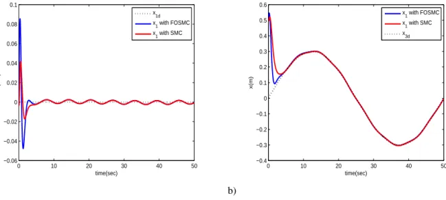
Figure 3. Simulation results of case 1 without any disturbance, a) Angle evolutionθ, b) displacementx It can be seen from figures, thatx1 andx3 converge respectively to the desired trajectoriesx1d andx3d.
Also, the convergence of these states using the proposed FOSMC is faster than that of classical SMC, this is obtained under considerable magnitude ofx1and control signal (u) in the transition state for the first one. With adding external disturbance, the system is still stable.
5. CONCLUSION
In this paper a sliding mode control scheme based on fractional order calculus was proposed for a class of non-linear systems, which is characterized by a single input and two outputs (SITO). The proposed approach used two fractional order sliding surfaces with intermediate variable between them; in which the control law was calculated to control the two system outputs. The Lyapunov theorem is used to prove the stability condition. Finally the simulation
a) 0 5 10 15 −0.1 −0.05 0 0.05 0.1 0.15 0.2 0.25 0.3 0.35 time(sec) z with SMC with FOSMC b) 0 5 10 15 −4 −2 0 2 4 6 8 time (sec) u (N) with SMC with FOSMC
Figure 4. Simulation results of case 1 without any disturbance, a) intermediate variable z, b) control signal u
a) 0 5 10 15 −0.06 −0.04 −0.02 0 0.02 0.04 0.06 0.08 0.1 time(sec) θ (rad) x 1with SMC x1d x 1with FOSMC b) 0 5 10 15 −0.1 0 0.1 0.2 0.3 0.4 0.5 0.6 time(sec) x (m) with SMC x 3d with FOSMC
Figure 5. Simulation results of case 1 with adding external disturbance, a) Angle evolutionθ, b) displacementx
for inverted pendulum system have shown that the proposed FOSMC give the best control specification compared with the conventional one based on integer order.
REFERENCES
[1] V. I. Utkin, ”Sliding modes and their applications in variable structure systems”.Mir, Moscow. 1978. [2] J. J .E. Slotine, W. Li, ”Applied nonlinear control”,Prentice-Hall, USA, 1991.
[3] J-J. Wang, ”Simulation studies of inverted pendulum based on PID controllers”, Simulation Modelling Practice and Theory, vol. 19, pp. 440-449, 2011.
[4] L-B. Prasad, B. Tyagi, H-O. Gupta, ”Modelling Simulation for Optimal Control of Nonlinear Inverted Pendulum Dynamical System using PID Controller LQR”,Sixth Asia Modelling Symposium, pp. 138-143, 2012.
[5] S-K. Oh, W. Pedrycz, S-B. Rho, T-C. Ahn, ”Parameter estimation of fuzzy controller and its application to inverted pendulum”,Engineering Applications of Artificial Intelligence, vol. 17, pp. 37-60, 2004.
[6] A-M. El-Nagar, M-El-Bardini, N-M. EL-Rabaie, ”Intelligent control for nonlinear inverted pendulum based on interval type-2 fuzzy PD controller”,Alexandria Engineering Journal, vol. 53, pp. 23-32, 2014.
a) 0 5 10 15 −0.1 −0.05 0 0.05 0.1 0.15 0.2 0.25 0.3 0.35 time(sec) z with SMC with FOSMC b) 0 5 10 15 −4 −2 0 2 4 6 8 time(sec) u (N) with SMC with FOSMC
Figure 6. Simulation results of case 1 with adding external disturbance, a) intermediate variable z, b) control signal u
a) 0 10 20 30 40 50 −0.06 −0.04 −0.02 0 0.02 0.04 0.06 0.08 0.1 time(sec) θ (rad) x 1 with SMC x 1d x 1 with FOSMC b) 0 10 20 30 40 50 −0.4 −0.3 −0.2 −0.1 0 0.1 0.2 0.3 0.4 0.5 0.6 time(sec) x (m) x 3 with SMC x 3d x 3 with FOSMC
Figure 7. Simulation results of case 2 without any disturbance, a) Angle evolutionθ, b) displacementx
[7] M-J. Mahmoodabadi, S-A. Mostaghim, A. Bagheri, N. Nariman-zadeh, ”Pareto optimal design of the decoupled sliding mode controller for an inverted pendulum system and its stability simulation via Java programming”, Mathematical and Computer Modelling, vol. 57, pp. 1070-1082, 2013.
[8] J-C. Lo and Y-H. Kuo, ”Decoupled Fuzzy Sliding-Mode Control”,IEEE transactions on fuzzy systems, vol. 6, NO. 3, pp. 426-435, August 1998.
[9] Y-H. Chang, C-W. Chang, C-W. Tao, H-W. Lin, J-S. Taur, ”Fuzzy sliding-mode control for ball and beam system with fuzzy ant colony optimization”,Expert Systems with Applications, vol. 39 pp. 3624-3633, 2012.
[10] L-C. Hung, H-Y. Chung, ”Decoupled sliding-mode with fuzzy-neural network controller for nonlinear systems”, International Journal of Approximate Reasoning, vol.46, pp. 74-97, 2007.
[11] A. Oustaloup, ”Linear feedback control systems of fractional order between 1 and 2,”IEEE Int. Symp. Circ. Systems, Chicago, IL (1981).
[12] A. Oustaloup, ”The CRONE control,”ECC91, vol. 1, Grenoble, France, 1991.
[13] I. Podlubny, ”Fractional-order systems and PID-controllers”, IEEE Trans. Autom. Control, vol. 44, No. 1, pp.208-214, 1999.
a) 0 10 20 30 40 50 −0.1 −0.05 0 0.05 0.1 0.15 0.2 0.25 0.3 0.35 time(sec) z with SMC with FOSMC b) 0 10 20 30 40 50 −8 −6 −4 −2 0 2 4 6 8 time(sec) u (N) with SMC with FOSMC
Figure 8. Simulation results of case 2 without any disturbance, a) intermediate variable z, b) control signal u
a) 0 10 20 30 40 50 −0.06 −0.04 −0.02 0 0.02 0.04 0.06 0.08 0.1 time(sec) θ (rad) x 1d x 1 with FOSMC x 1 with SMC b) 0 10 20 30 40 50 −0.4 −0.3 −0.2 −0.1 0 0.1 0.2 0.3 0.4 0.5 0.6 time(sec) x(m) x 1 with FOSMC x 1 with SMC x 3d
Figure 9. Simulation results of case 2 with adding external disturbance, a) Angle evolutionθ, b) displacementx
tuning based on integral performance indices”, Engineering Applications of Articial Intelligence, vol. 25, pp. 430-442, 2012.
[15] A.J. Caldern, B. M. Vinagre, V. Feli, ”Fractional Sliding Mode Control of a DC-DC Buck Converter with Appli-cation to DC Motor Drives”,The11thInternational Conference on Advanced Robotics, Coimbra, Portugal, pp. 252-257, June 30 - July 3, 2003.
[16] A.J. Calderon, B.M. Vinagre, V. Feliu, ”Fractional order control strategies for power electronic buck converters”, Signal Processing, vol. 86, pp. 2803-2819, 2006.
[17] J. Huang, H. Li, Y. Chen, and Q. Xu, ”Robust Position Control of PMSM Using Fractional-Order Sliding Mode Controller”,Hindawi Publishing Corporation Abstract and Applied Analysis, vol. 2012.
[18] N. Bouarroudj, D. Boukhetala and F. Boudjema, ”A Hybrid Fuzzy Fractional Order PID Sliding-Mode Controller design using PSO algorithm for interconnected Nonlinear Systems”,CEAI, vol.17, No. 1, pp. 41-51, 2015. [19] H. Delavari, R. Ghaderi, A. Ranjbar, S. Momani, ”Fuzzy fractional order sliding mode controller for nonlinear
systems”,Commun Nonlinear Sci Numer Simulat, vol. 15 pp. 963-978, 2010.
[20] B. Zhang, Y. Pi, Y. Luo, ”fractional order sliding-mode control based on parameters auto-tuning for velocity control of permanent magnet synchronous motor”,ISA Transactions, vol. 51, pp. 649-656, 2012.
a) 0 10 20 30 40 50 −0.05 0 0.05 0.1 0.15 0.2 0.25 0.3 0.35 time(sec) z with FOSMC with SMC b) 0 10 20 30 40 50 −8 −6 −4 −2 0 2 4 6 8 time(sec) u (N) with FOSMC with SMC
Figure 10. Simulation results of case 2 with adding external disturbance, a) intermediate variable z, b) control signal u
[21] S. Dadras, H-R. Momeni, ”Fractional terminal sliding mode control design for a class of dynamical systems with uncertainty”,Commun Nonlinear Sci Numer Simulat, vol. 17 pp. 367-377, 2012.
[22] K. Oldham and J. Spanier. ”The fractional calculus: Theory and application of differentiation and integration to arbitrary order”.Wiley, NewYork, 1974.
[23] S. Miler, ”introduction to the fractional calculus and fractional differential equations”.Wiley, New York, 1993. [24] I. Podlubny, ”Fractional Differential Equations”, Mathematics in Science and Engineering, vol. 198.San Diego:
Academic Press, 1999.
[25] M.D. Ortigueira, J.J. Trujillo, ”Generalized GL Fractional Derivative and its Laplace and Fourier Transform”, Proceedings of the ASME 2009,International Design Engineering Technical Conferences Computers and Infor-mation in Engineering Conference, IDETC/CIE 2009.
[26] A. Oustaloup, F. Levron, B. Mathieu, F. M. Nanot, ”Frequency-band complex noninteger differentiator: charac-terization and synthesis”,IEEE Transactions on Circuits and Systems I: Fundamental Theory and Applications, vol. 47, Issue: 1, pp. 25-39, 2000.