Trace: Tennessee Research and Creative
Exchange
Masters Theses
Graduate School
12-2011
Potential Impacts of Climate Change on Water
Resources and Water Quality of Norris Lake,
Tennessee
Yong-Gil Choi
[email protected]This Thesis is brought to you for free and open access by the Graduate School at Trace: Tennessee Research and Creative Exchange. It has been accepted for inclusion in Masters Theses by an authorized administrator of Trace: Tennessee Research and Creative Exchange. For more information, please [email protected].
Recommended Citation
Choi, Yong-Gil, "Potential Impacts of Climate Change on Water Resources and Water Quality of Norris Lake, Tennessee. " Master's Thesis, University of Tennessee, 2011.
I am submitting herewith a thesis written by Yong-Gil Choi entitled "Potential Impacts of Climate
Change on Water Resources and Water Quality of Norris Lake, Tennessee." I have examined the final
electronic copy of this thesis for form and content and recommend that it be accepted in partial
fulfillment of the requirements for the degree of Master of Science, with a major in Environmental
Engineering.
Randall W. Gentry, Ungtae Kim, Major Professor
We have read this thesis and recommend its acceptance:
Jack C. Parker
Accepted for the Council:
Carolyn R. Hodges
Vice Provost and Dean of the Graduate School
(Original signatures are on file with official student records.)
Resources and Water Quality of Norris Lake, Tennessee
A Thesis Presented for
the Master of Science
Degree
The University of Tennessee, Knoxville
Yong-Gil Choi
December 2011
Copyright © 2011 by Yong-Gil Choi All rights reserved.
Acknowledgements
Foremost I would like to thank Dr. Ungtae Kim and Dr. Randall Gentry for serving as my major advisors. They have helped me since I first arrived at the University of Tennessee and have made this study possible. I also would like to express my gratitude to Dr. Jack Parker for sitting on my committee and his encouragement and professional guidance throughout this study and my graduate career.
This study would not have been possible without the data provided by the Intergovernmental Panel on Climate Change (IPCC), the U.S. Geological Survey (USGS), the National Land Cover Data (NLCD), the National Climatic Data Center (NCDC), the U.S. Environmental Protection Agency (EPA), and the Tennessee Valley Authority (TVA).
My sincere thanks also go to Hun Ju Yi, Woon Cho, Jacob D’avy and Yesle Yi for cheering and supporting me. Last but not least, I would like to thank my parents Duk-Chul Choi and Ok-Soon Chang; my parents-in-law Il-Hee Park and Yeon-Suk Bae; brothers and sisters; and finally my lovely wife Sookyung Park.
Abstract
This study assessed the potential impacts of climate change on hydrology, water resources operation, and water quality of the Norris Lake area in Tennessee. To project future climate conditions, the simulation outputs for 2030s, 2050s, and 2070s from six general circulation models (GCMs) were extracted under two Intergovernmental Panel on Climate Change (IPCC) greenhouse gases emissions scenarios (A2 and B1 for high and low emissions, respectively) to consider the range of uncertainty. The outputs of the six GCMs were weighted by considering their accuracy to simulate the climate conditions observed from 1961 to 1990 to suggest an ensemble average. A water balance model was calibrated to the observed hydrologic monitoring data and this calibrated model was used to simulate the runoff for different climate conditions. Flow duration curves in lieu of hydrologic regime were constructed from the generated runoff hydrographs and the percent changes of flow statistics representing drought, flood, and normal seasons were suggested for the future. Finally, the operational performance of Norris Dam under the projected climate conditions was evaluated by the quantitative indices, reliability, resilience, and vulnerability (RRV). The results suggest that future temperature and precipitation for the 2050s are expected to increase about 1.3ºC and 5.7%, respectively, based on the weighted GCMs. The probability of flood and drought is likely to increase in the presence of uncertainty of runoff generated using multi-GCMs and emissions scenarios. The weighted results suggest the improved RRV in the 2050s, implying the future inflows to Norris Dam meet the future dam operation requirement. However, based on the weighted scenario for the 2050s, the future stream temperature shows a slight increase (annually about +1oC) and the concentration of dissolved oxygen shows an about 1 mg/L drop for the summer seasons. This minor deterioration of water quality is mainly due to the expected increase of air temperature in the future. The major findings and results of this study provide decision-makers and engineers with guidelines for evaluating the potential impacts of climate change on water resources systems of the Norris Lake area.
Table of Contents
Chapter 1 Introduction and Literature Review ... 1
Chapter 2 Materials and Methods ... 6
2.1 Information of the Study Area ... 6
2.1.1 Upper Clinch River, Powell River Basins, and Norris Dam ... 6
2.1.2 Land Cover ... 9
2.1.3 Climate and Hydrology ... 10
2.2 Future Climate Change Scenarios ... 11
2.2.1 Future Greenhouse Gas Emissions Scenarios ... 11
2.2.2 General Circulation Models ... 12
2.3 Water Balance Model and Generation of Climate Variables ... 14
2.3.1 Water Balance Model ... 14
2.3.2 Generation of Climate Variables ... 16
2.4 Evaluation of Hydrologic Regimes and Water Resources system ... 17
2.4.1 Hydrologic Regimes ... 17
2.4.2 Reliability, Resilience, and Vulnerability (RRV) ... 17
2.5 Water Quality Model ... 19
Chapter 3 Results and Discussions... 21
3.1 Climate Change Scenarios ... 21
3.1.1 Base Case Climate Scenario ... 21
3.1.2 Future Climate Scenarios ... 21
3.2 Runoff Generation ... 28
3.2.1 Calibration and Validation ... 28
3.2.2 Runoff Generation for Climate Scenarios... 29
3.3 Hydrologic Regimes and Performance of Dam Operation ... 30
3.3.1 Changes of Flow Duration ... 31
3.3.2 Performance Evaluation of Dam Operation ... 33
3.4 Water Quality ... 35
3.4.1 Steam Temperature ... 35
3.4.2 DO Concentration ... 37
Chapter 4 Summary, Conclusions and Recommendations ... 39
List of References ... 42
List of Tables
Table 1 Land Use for Powell and Upper Clinch Basins (NLCD, 2001) ... 9
Table 2 Description of the Selected GCMs ... 13
Table 3 Comparison of Statistics between the Observed and Generated Time-Series ... 22
Table 4 Comparison of the Observed and GCM Simulated Climate Data for 1961 to 1990 ... 23
Table 5 Weighting Factors for Six GCMs ... 25
Table 6 Changes of Climate Variables for the 2050s under the A2 Emission Scenario ... 26
Table 7 Changes of Climate Variables for the 2050s under the B1 Emission Scenario ... 27
Table 8 Average Percent Changes of Flow Statistics for Two Emissions Scenarios ... 33
Table 9 Changes of Reliability, Resilience, and Vulnerability of Future Dam Operation using WEIGHT ... 34
List of Figures
Figure 1 Conceptual Research Scheme ... 5
Figure 2 Map Showing the Locations of Norris Dam, Weather, Streamflow, and Water Quality Monitoring Sites ... 6
Figure 3 Norris Dam, Tennessee ... 7
Figure 4 Example of Norris Dam Operating Guide (TVA, 2011) ... 8
Figure 5 Monthly Mean Air Temperature and Precipitation (1970-2005) ... 10
Figure 6 Conceptual Water Balance Model with Two Soil Layers (Kim and Kaluarachchi, 2009) ... 14
Figure 7 Calibration and Validation of the Water Balance Model ... 28
Figure 8 Percent Changes of Runoff for Different Emissions Scenarios and Time Periods using WEIGHT ... 29
Figure 9 Comparison of Flow Duration Curves for Different Emission Scenarios and Time Periods ... 32
Figure 10 Monthly Mean Air and Stream Temperature observed from 1997 to 2010 ... 35
Figure 11 Relationship between Air Temperature and Stream Temperature measured at Cleveland, VA ... 36
Figure 12 Mean Changes of Stream Temperature Projected for Different Emissions Scenarios and Time Periods using WEIGHT ... 37
Figure 13 Relationship between Stream Temperature and DO Concentrations obtained from EPA STORET ... 37
Figure 14 Monthly Mean DO Concentration Projected for Different Emissions Scenarios and Time Periods using WEIGHT ... 38
Chapter 1
Introduction and Literature Review
The World Meteorological Organization (WMO) reported that the global average surface temperature has risen about 0.7°C since the beginning of the 20th century; but this rise has not been purely linear. The global average temperature has risen sharply at 0.18°C per decade from the late 1970s. In the northern and southern hemispheres, the 1990s were the warmest decade with an average of 0.38°C and 0.23°C above the 30-year mean, respectively (WMO, 2005). Moreover, according to the 2009 WMO report regarding the warmest decade, the 2000s was warmer than the decade spanning the 1990s (WMO, 2009). The 10 warmest years for the earth’s surface temperature all occurred after 1990, and 2005 was the warmest year on record (Jones and Palutikof, 2006; Hansen et al., 2006).
Much of the warming during the last four decades is attributable to the increasing atmospheric concentrations of greenhouse gases (GHGs) due to human activities (Santer et al., 1996; Tett et al., 1999; Meehl et al., 2003; Cayan et al., 2008). This global warming has been strongly linked to changes in the global hydrological cycle such as increases of atmospheric water vapor resulting in changes of precipitation patterns, intensity, and extremes; reduced snow cover and the widespread melting of ice; and changes in soil moisture and runoff. These impacts on water quantity and quality due to climate change are expected to affect the function and operation of existing water infrastructures including hydropower, structural flood defenses, drainage, and irrigation systems, as well as water management practices (IPCC, 2008).
According to the 4th assessment report (AR4; IPCC, 2007) and special report on emissions scenarios (SRES; IPCC, 2000) of the Intergovernmental Panel on Climate Change (IPCC) based on atmosphere-ocean general circulation model simulations, the projected global
mean temperature for the SRES B1, a moderate-emission scenario, is projected to rise about 1.8°C (1.1°C to 2.9°C) by 2100. For a higher-emission scenario, the SRES A2, the global mean temperature is projected to rise about 3.4°C (2.0°C to 5.4°C) by 2100. The current outputs of GCMs indicate that the precipitation generally increases in the areas of regional tropical precipitation maxima (such as the monsoon regimes) and over the tropical Pacific in particular, with general decreases in the subtropics, and increases at high latitudes as a consequence of a general intensification of the global hydrological cycle. Globally averaged mean water vapor, evaporation, and precipitation are projected to increase. Also, the intensity of the precipitation events is projected to increase, particularly in tropical and high latitude areas that experience increases in mean precipitation.
Analyzing possible impacts of climate change on watershed environments using the outputs of GCMs have become a major topic of many recent studies. Palmer and Räisänen (2002) projected a considerable increase in the risk of a very wet winter over much of central and northern Europe due to an increase in intense precipitation associated with mid-latitude storms. Mirza (2003) projected that the area typically flooded in Bangladesh could increase by at least 23% with a global temperature rise of 2°C. To quantify the climate change impacts on watershed hydrology, many previous studies combined water balance models, which provide simple and reliable watershed runoff simulation, with the projected future climate outputs from GCMs (e.g., Conway, 1997; Yates and Strzepek, 1998; Xu, 2000; Wanchang et al., 2000; Folwer et al., 2003; Wurbs et al., 2005; Kim and Kaluarachchi, 2009). The change of available water resources due to climate change can alter the robustness of water resources systems (e.g., water allocation systems, hydropower sites, etc.). Increased stream temperatures with increased air temperature by global warming and changes in the hydrological cycle are projected to affect water quality and exacerbate many forms of water pollution such as sediments, nutrients, pathogens, pesticides and
salt, as well as thermal pollution, which could possibly affect ecosystems, human health, and water system reliability and operating costs (Roy et al., 2005; IPCC, 2007 and 2008).
As described above, climate change affects various areas of watershed environment and management. A large watershed having an integrated resource management system such as the Tennessee Valley Authority (TVA) is particularly subject to impacts from climate change. EPA (1999) summarized the probable impacts of climate change on watershed hydrology and the water system in the Tennessee areas. Based on EPA (1999), snow accumulation is minimal in Tennessee and runoff would be influenced primarily by higher temperatures, increased evaporation, and precipitation changes. As a result of those factors, hydropower generation could be influenced, navigation disrupted, recreational opportunities degraded, and water availability for water supplies reduced if the runoff decreases. On the other hand, if rainfall and runoff increase in the Tennessee region, then higher streamflows and lake levels could benefit hydropower production, enhance recreational opportunities, and improve water availability for water supplies. Increased rainfall also could increase flooding, which is currently a problem in the steep terrain of eastern Tennessee, along the many unregulated streams throughout the state, and in growing urban areas (EPA, 1999). The future changes of the water quantity and quality caused by the climate change could influence human activities and the ecosystem over the TVA area.
These assumptions emphasize the necessity to evaluate the climate change impacts on water resources and environments of the TVA area. However, although there have been many climate change studies in the United States, little attention has been paid to the climate change impact on the watersheds of the TVA area. From this point of view, this study aims to evaluate future changes in watershed hydrology, water resources operation, and water quality of the TVA area under different future IPCC SRES greenhouse gas emissions scenarios. This study chooses the Upper Clinch River basin as a case study, where the Norris Dam, the first TVA multi-purpose
dam built in 1936, is located. The specific objectives and tasks to achieve this goal can be summarized as follows:
1. Develop a theoretical framework to assess the future variability of hydrologic conditions of the study area under different climate change scenarios.
- Collect multiple GCMs outputs under different GHGs emissions scenarios to consider uncertainty.
- Extract baseline climate data from each GCM.
- Construct long-term multiple sets of future climate change data for 2030s, 2050s, and 2070s.
2. Simulate watershed runoff using a water balance model.
- Calibrate a water balance model using the observed hydrologic data. - Simulate future runoff using the baseline and projected future climate data.
3. Assess the possible impacts of climate change on regional water resources. - Evaluate the future changes of hydrologic regimes (flow duration curves)
- Evaluate the future changes of the performance of dam operation using criteria and indices.
4. Evaluate future water quality.
- Develop regression models to correlate air temperature, stream temperature, and dissolved oxygen concentration using observed data.
5. Provide recommendations for future basin management.
- Suggest average changes of watershed hydrology, water resources operation, and water quality with uncertainty for future decision-making.
- Recommend future research directions.
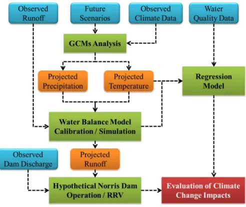
The conceptual framework of this study is depicted in Figure 1.
Chapter 2 Materials and Methods
2.1 Information of the Study Area
2.1.1 Upper Clinch River, Powell River Basins, and Norris Dam
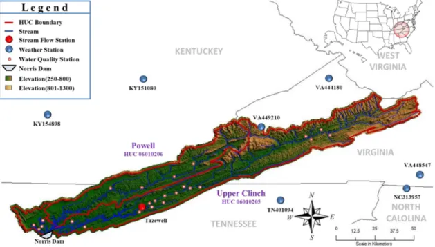
The Upper Clinch (Hydrologic Unit Code (HUC): 06010205) and the Powell River (HUC: 06010206) watersheds are located in Western Virginia and Eastern Tennessee and are parts of the Tennessee Big Sandy River Basin. The drainage areas are 5,125 square kilometers for the Upper Clinch River Basin and 2,435 square kilometers for the Powell River Basin. Both basins are all the water sources of Norris Lake as shown in Figure 2.
Figure 2. Map Showing the Locations of Norris Dam, Weather, Streamflow, and Water Quality Monitoring Sites.
The Clinch River runs from Southwest Virginia near Tazewell, Virginia and flows southwest through the Great Appalachian Valley, gathering various tributaries including the Powell River before joining the Tennessee River in East Tennessee. The Clinch River includes two dams: Norris Dam, the first dam built by the TVA; and Melton Hill Dam, the only TVA dam with a lock not located on the main channel of the Tennessee River.
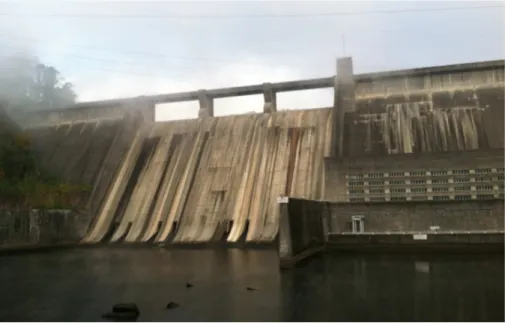
Norris Dam is located at the ends of Powell River and Upper Clinch River and discharges into Lower Clinch River. It is a multipurpose dam of hydropower generation, water supply, and drought and flood control (Figure 3). Norris Dam is 265 feet high and stretches 1,860 feet across the Clinch River.In a year with normal rainfall, the water level in Norris Reservoir varies about 29 feet from summer to winter to provide seasonal flood storage. The reservoir has a flood-storage capacity of 1,113,000 acre-feet. The hydroelectric power plant at Norris Dam consists of two generating units, each of which has 4,800 ft3/sec of maximum runoff (TVA, 1940).
Norris Lake, the largest reservoir on a tributary of the Tennessee River, with 809 miles of shoreline and 33,840 acres of water surface, is a popular tourist and recreation destination. In the 1930s, TVA established demonstration public parks at several locations on Norris Reservoir, including Cove Lake, Big Ridge, and the areas around Norris Dam. These parks later became the nucleus of Tennessee’s state park system supporting various recreation activities including hiking, boating, water skiing, swimming, and excellent fishing. Moreover, Norris Lake has various aquatic habitats in the watershed, and the Clinch River including the Powell River has one of the most diverse fish and mussel faunas in North America as Eckert (2010) documented that 20% of the 300 species in the U.S. are known from the Clinch River.
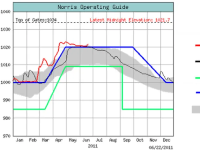
To evaluate the operational performance of water resources systems of the study area, the current operating and management rules of Norris Dam were needed. Although the specific operating rules for each month or seasons are not sufficient for Norris Dam, TVA has provided the basic operating elevation guides as shown in Figure 4 and also provided the hourly dam discharge data from 1936 to 2010. Using the averages of monthly dam discharge data as evaluation criteria for dam operation, the reservoir can be routed using long-term monthly inflow time-series.
2.1.2 Land Cover
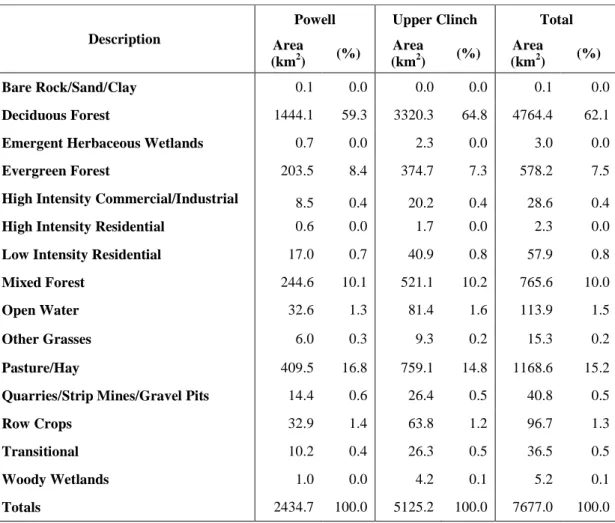
The land cover data of Powell and Upper Clinch basin obtained from the National Land Cover Data (NLCD) did not show any significant difference between 1992 and 2001, implying the impacts of land use change on runoff are negligible, compared to those by climate change. As shown in Table 1, the most portions of the land use are forest (79.6%) and pasture/hay (15.2%), while the impervious area is below 3%. This study assumed, therefore, that significant changes of the land cover are not expected and the land cover of the study area will barely change because no projected development in the watershed has been reported.
Table 1. Land Use for Powell and Upper Clinch Basins (NLCD, 2001)
Description
Powell Upper Clinch Total Area (km2) (%) Area (km2) (%) Area (km2) (%) Bare Rock/Sand/Clay 0.1 0.0 0.0 0.0 0.1 0.0 Deciduous Forest 1444.1 59.3 3320.3 64.8 4764.4 62.1
Emergent Herbaceous Wetlands 0.7 0.0 2.3 0.0 3.0 0.0
Evergreen Forest 203.5 8.4 374.7 7.3 578.2 7.5
High Intensity Commercial/Industrial 8.5 0.4 20.2 0.4 28.6 0.4 High Intensity Residential 0.6 0.0 1.7 0.0 2.3 0.0
Low Intensity Residential 17.0 0.7 40.9 0.8 57.9 0.8
Mixed Forest 244.6 10.1 521.1 10.2 765.6 10.0
Open Water 32.6 1.3 81.4 1.6 113.9 1.5
Other Grasses 6.0 0.3 9.3 0.2 15.3 0.2
Pasture/Hay 409.5 16.8 759.1 14.8 1168.6 15.2
Quarries/Strip Mines/Gravel Pits 14.4 0.6 26.4 0.5 40.8 0.5
Row Crops 32.9 1.4 63.8 1.2 96.7 1.3
Transitional 10.2 0.4 26.3 0.5 36.5 0.5
Woody Wetlands 1.0 0.0 4.2 0.1 5.2 0.1
2.1.3 Climate and Hydrology
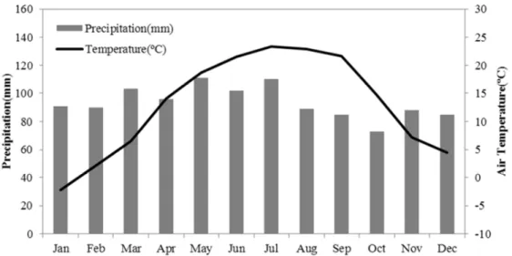
The climate of the study area can be defined as humid subtropical with hot and moist summers and mild winters (Parker, 2008; NCDC, 2010). Most summer rainfall occurs during thunderstorms and occasional tropical storms. Early summer and spring typically have the most abundant precipitation. The early fall is usually the driest season due to slow-moving high pressure systems. Winter precipitation is usually rainfall, occasionally snowfall, and is associated with large-scale frontal systems lasting for longer time. January is the coldest month averaging near -2°C, and July is the warmest with an average temperature near 23°C (Figure 5).
In general, most of the study area evenly receives abundant precipitation throughout the year. Dry periods usually occur during the summer and fall and may last for weeks at a time. Heavy and prolonged precipitation can cause periods of widespread flooding and local floods during the winter and early spring. Heavy downpours from summer thunderstorms frequently cause local flooding (NCDC, 2010).
Observed precipitation and temperature data from 1970 to 2005 were gathered from an EPA meteorological database (EPA, 2006). These weather stations are located in similar latitude around the study area (Figure 2) and the differences of the weather data are not significant, so it can be assumed that the averaged climate data of the stations can represent the climate of the entire watershed. The streamflow data of Tazewell, Tennessee from 1936 to 2010 were obtained from the United States Geological Survey (USGS, 2011) for the model calibration.
2.2 Future Climate Change Scenarios
2.2.1 Future Greenhouse Gas Emissions Scenarios
Many international modeling groups have completed simulations of present and future climate under the SRES scenarios in preparation for the IPCC 4th Assessment Report (AR4; IPCC, 2007). Among the 40 scenarios under the four storylines (A1, A2, B1, and B2 families) described in the SRES, the marker emission scenarios selected from individual families provide bases that relates emissions to driving forces of climate simulation models (IPCC, 2000). Therefore, the outputs of GCMs used in this study were based on the marker emissions scenarios.
The marker A2 scenario (A2), for example, assumes that global CO2 emissions continue
to climb throughout the century, reaching almost 30 gigatons per year (Gt/year). By the end of the twenty first century, CO2 concentrations reach more than triple their pre-industrial levels. This
yields a doubling of CO2 concentrations relative to its pre-industrial level by the end of the
century, followed by a leveling of the concentrations. Under the marker B1 scenario (B1), CO2
emissions will peak at approximately 10 Gt/year in the mid-twenty-first century before dropping below current levels by 2100 (Cayan et al., 2008).
Although A2 does not represent the highest CO2 emissions among the SRES scenarios
(Beyene et al., 2009). As such, although it is by no means a “worst case,” A2 represents the higher emission case commonly used to represent the maximum emission case in climate studies, and thus was used in this study. B1 generally represents the most positive case of the SRES scenarios through the twenty first century (IPCC, 2000). Therefore, the marker A2 and B1 scenarios were reasonable to establish the impact ranges (maxima and minima) of the climate changes. A GCM baseline scenario, called the 20C3M from which the projected future climate data were modeled, is the experimental run with the GHGs increasing as observed through the 20th century. The 20C3M output for each climate model can be used as a benchmark to determine changes of the future climate projection results (Cayan et al., 2008).
2.2.2 General Circulation Models
GCMs are mathematical representations of atmospheric, oceanic, and continental processes and interactions. These models are limited by complexity and uncertainty as well as non-linear interactions among atmospheric and oceanic processes (Hillel and Rosenzweig, 1989). Although there are many GCMs involved in the AR4 of the IPCC, this study assumed that the GCMs developed at the North America would show higher accuracy on that area than other GCMs. Six GCMs were finally selected (Table 2): the Coupled Global Climate Model 3 (CGCM3, Canadian Centre for Climate Modelling and Analysis (CCCma)), the Geophysical Fluid Dynamics Laboratory (GFDL) CM2.0 and CM2.1 models (CM2.0 and CM2.1, GFDL), Goddard Institute for Space Studies E-R (GISS-E-R from National Oceanic and Atmospheric Administration (NOAA) of National Aeronautics and Space Administration (NASA)), and the Parallel Climate Model and Community Earth System Model (PCM and CCSM from National Center for Atmospheric Research (NCAR) and Department of Energy (DOE), respectively).
Table 2. Description of the Selected GCMs
GCM Country Resolution a Temporal Coverage Number of Grids b
CCCma-CGCM3 Canada 96 × 48 16/1/2001 - 16/12/2100 2 GFDL-CM2.0 U.S.A 144 × 90 16/1/2001 - 16/12/2100 2 GFDL-CM2.1 U.S.A 144 × 90 16/1/2001 - 16/12/2100 2 GISS-E-R U.S.A 72 × 46 16/1/2004 - 16/12/2100 1 NCAR-PCM U.S.A 128 × 64 16/1/2000 - 16/12/2099 3 NCAR-CCSM U.S.A 256 × 128 16/1/2000 - 16/12/2099 5 a: Mean resolution of GCMs in longitude and latitude
b: The number of grids covering the study area
The 20C3M conditions used in the selected models accounted for historical inputs into the atmosphere of aerosols from volcanic eruptions, changes in solar irradiance, and anthropogenic GHGs and aerosol loadings (Meehl et al., 2003; Delworth et al., 2006). The results of the modeled climate from 1961 to 1990 were used as climatology, a benchmark to which future-climate simulations were compared. The modeled climate variables from 1961 to 1990 can also be compared to the observed climate data for the same period to evaluate the accuracy of each GCM in simulating the current climate conditions. To find an ensemble average of the six selected GCMs outputs, a weighing factor for each GCM was computed by the inverse of the mean absolute error between historic climate data and 20C3M simulated climate data of each GCM.
The gridded GCMs outputs under two emission scenarios for future and baseline were obtained from the IPCC Data Distribution Center (DDC) (IPCC, 2010). The future climate variables for the 2030s (mean of 2020 to 2039), 2050s (mean of 2040 to 2059), and 2070s (mean of 2060 to 2079) were projected by perturbing the current climate variables using the GCMs’ climate variable data for each corresponding time period.
2.3 Water Balance Model and Generation of Climate Variables 2.3.1 Water Balance Model
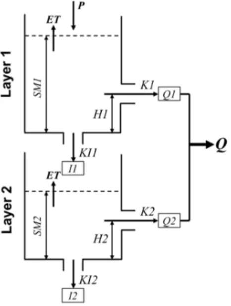
The hydrologic model used in this study is a two-layer water balance model, which has a relatively simple yet reliable soil moisture accounting structure. Several variations of the model have been widely used in simulating runoff dynamics of various basins in the world (Sugawara, 1995; Yokoo et al., 2001; Chen et al., 2005; Cooper et al., 2007; Kim et al., 2008). The proposed model computes monthly runoff using monthly precipitation (P) and potential evapotranspiration (PET) over the study area by updating two soil moisture storages at each monthly time step. The conceptual scheme of the water balance model is described in Figure 6 and its numerical implementation is as follows.
Figure 6. Conceptual Water Balance Model with Two Soil Layers (Kim and Kaluarachchi, 2009).
The runoff (Qi) at time t from the ith soil layer is computed by
where Ki is the coefficient of runoff in the ith soil layer and Hi is the height of the ith runoff orifice.
The infiltration (Ii) at time from the ith soil layer is computed by
Ii(t)= KIi·SMi(t) (2)
where KIi is the coefficient of infiltration in the ith soil layer.
Actual evapotranspiration ETi(t) at time t is computed by the following (Dingman, 2002). ET(t) = P(t) / [ 1 + {P(t) / PET(t)}2 ]1/2 (3) where PET(t) is potential evapotranspiration at time t. This relationship was suggested by Kim (2007) instead of other methods considered by Johnson and Curtis (1994) and Arnell and Reynard (1996) due to its better performance in simulating the observed hydrographs. Note that ET(t) at the 2nd soil layer is computed only when the soil moisture in the 1st soil layer is deficient (Kim, 2007).
Soil moisture (SMi) of the each layer is then updated by accounting in-and-out water at each time step t. Finally, the total runoff (Q) at time t from the basin is Q(t) = Q1(t) + Q2(t).
As Eqs. (1) to (2) describe that the simulated total runoff is controlled by the coefficients of runoff (Ki) and infiltration (KIi) and the height of orifice (Hi), this study calibrates those model parameters using genetic algorithms (GAs), one of the most well-known numerical optimization algorithms in various engineering practices. Because the linear combination of each runoff component can produce highly nonlinear behavior (Yokoo et al., 2001; Chen et al., 2005), it can be assumed that the six model parameters of the water balance model are adequate to represent the monthly water balance of the study area.
The 36-year monthly precipitation, temperature, and runoff data from 1970 to 2005 were used; 30 years for calibration and 6 years for validation. From a preliminary run, the 36 year mean values of soil moisture in January were set as the initial soil moisture conditions for a
reasonable low-bias starting condition. MATLAB, a general scientific programming language developed by MathWorks® (http://www.mathworks.com/), was used to calculate and calibrate the water balance model described above. The GA toolbox of MATLAB, a set of GA optimization functions, was applied to estimate the best parameters. The sum square error was selected as an objective function (F) that produces the best calibration performance in representing both low and high flow seasons of the study area, compared to other three objective functions (log-transformed error, square root transformed error, and relative error).
4 where t is time step from 1 to T; Qobs is the observed value, and Qsim is the simulated value.
The Nash-Sutcliffe (NS) coefficient defined by Nash and Sutcliffe (1970) was used as a measure of agreement between observed and simulated values.
NS 1 ∑∑ 5
2.3.2 Generation of Climate Variables
Since the data lengths of observed climate variables were too short to capture whole the ranges of randomness, the data should be augmented. This study used the conditional generation method (CGM) proposed by Kim et al. (2008) among various generation methods to generate monthly precipitation and temperature from the observed data because CGM has a capability to preserve the temporal and spatial correlations between adjacent time steps or locations. More detailed methods can be found in Kim et al. (2008).
The evaluation of long-term behavior of a water resources system (e.g., dam operation) especially requires a sufficient length of time-series. For this purpose, this study reproduced 200-year time-series of climate variables (e.g., precipitation and temperature) using CGM.
2.4 Evaluation of Hydrologic Regimes and Water Resources system 2.4.1 Hydrologic Regimes
This study used flow duration curves as an indicator of the hydrologic regime of the study area. The flow duration curve is a statistically cumulative distribution function of daily, weekly, or monthly streamflow, which is widely used by hydrologists (Foster, 1934). Although it is a simple function, the flow duration curve can comprehensively show overall variability of flow in a watershed. The flow duration curves can be applied to many hydrologic studies such as evaluating hydropower generation, water supply, and irrigation (Chow, 1964; Warnick, 1984; Vogel and Fennessey 1994; Smarkhtin, 2001; Kim and Kaluarachchi, 2009).
The flow statistics, Q10, Q50, and Q90, which represent the streamflows exceeding the
probabilities of 10%, 50%, and 90%, respectively, were extracted from the flow duration curves under different future climate conditions. This study assumed that the Q10 and Q90 flows can
represent flood and drought conditions, and thus, the changes of Q10 and Q90 in future runoff can
imply the changes of flood and drought recurrence.
2.4.2 Reliability, Resilience, and Vulnerability (RRV)
The operational performance of a water resources system can be quantitatively expressed using a proper index. The indices of reliability, resilience, and vulnerability (RRV), originally proposed by Hashimoto et al. (1982), are generally used for classifying and evaluating the performance of water resources systems. Those indices have been applied to many studies to evaluate reservoir operations (Hashimoto et al., 1982; Moy et al., 1986), to evaluate water distribution systems (Zongxue et al., 1998), to manage the water quality of a river (Maier et al., 2001), and to assess climate change impacts on water resources systems (Fowler et al., 2003; Kim, 2007).
Reliability is a measure of the frequency or probability when a system is in a satisfactory state meeting a given criterion. Resilience generally indicates a measure of how quickly a system recovers from failure to a satisfactory state once failure has occurred. Vulnerability can be defined as the maximum duration of system failure and the cumulative maximum magnitude of water shortage in system failure. The mathematical expressions are as follows (Hashimoto et al., 1982; Fowler et al., 2003; Kim, 2007).
Monthly discharge (Xt) can be classified as the satisfactory or failure state (S or F) based
on the criterion C, which is the minimum required discharge from a reservoir for watershed management.
If Xt≥ C then Xt∈ S and Zt = 1 (6)
Else Xt∈ F and Zt = 0
where Zt is a generic binary indicator variable. The mean monthly runoff or dam outflow is
usually adopted as a criterion. Another indicator, Wt, which represents a transition from F to S, is
defined as
W 1, if X ∈ F and X) ∈ S
0, otherwise (7)
If the periods of Xt in F are defined as U1, U2, …, UN where N is the number of F periods,
then reliability, resilience, and vulnerability indices during the total time period (T) can be defined as Reliability ∑ 67 8 Resilience 7 ∑∑ :6 9 Vulnerability > Max A , A , AB, … , AD 10 VulnerabilityE FG > MaxH I J , K ∈LM 1,2,3, … , N P 11
This study assumed the observed mean monthly outflow of Norris Dam can be an evaluation criterion because outflow data includes both hydropower generation and minimum requirement for downstream ecology. Therefore, failure of dam operation occurs when the future outflow of a month is less than the mean outflow of that month.
2.5 Water Quality Model
The study area does not have maintained a large enough amount of water quality data to simulate a sophisticated water quality model for evaluating the impacts of the climate changes. Among several water quality monitoring data, stream temperature and dissolved oxygen (DO) concentration data were only available for this study.
Daily mean stream temperature data from 2007 to 2010 were obtained from the station of the USGS 03524000 near Cleveland, Virginia, measured by the Virginia Water Science Center (VWSC) of the USGS (USGS, 2011). The DO concentration data with additional stream temperature from 1997 to 2010 were obtained from the STORET (storage and retrieval) maintained by EPA (EPA, 2011). Although the data included several missing periods, the water quality data were sufficient to be correlated with air temperature data.
Regression methods have been widely used to drive the relationships among air temperature, stream temperature, and DO concentration because these methods do not require physical model parameters to calibrate (Pilgrim et al., 1998; Benyahya et al., 2007).
The general form of a regression model used in this study is
Y = a0 + a1X1 + a2X2 + … anXn (12)
where ai is a regression coefficient that can be estimated using the method of least squares
This study used air temperature or stream temperature data as an independent variable and its corresponding dependent variable was the stream temperature or DO concentration, respectively.
Chapter 3 Results and Discussions
3.1 Climate Change Scenarios
3.1.1 Base Case Climate Scenario
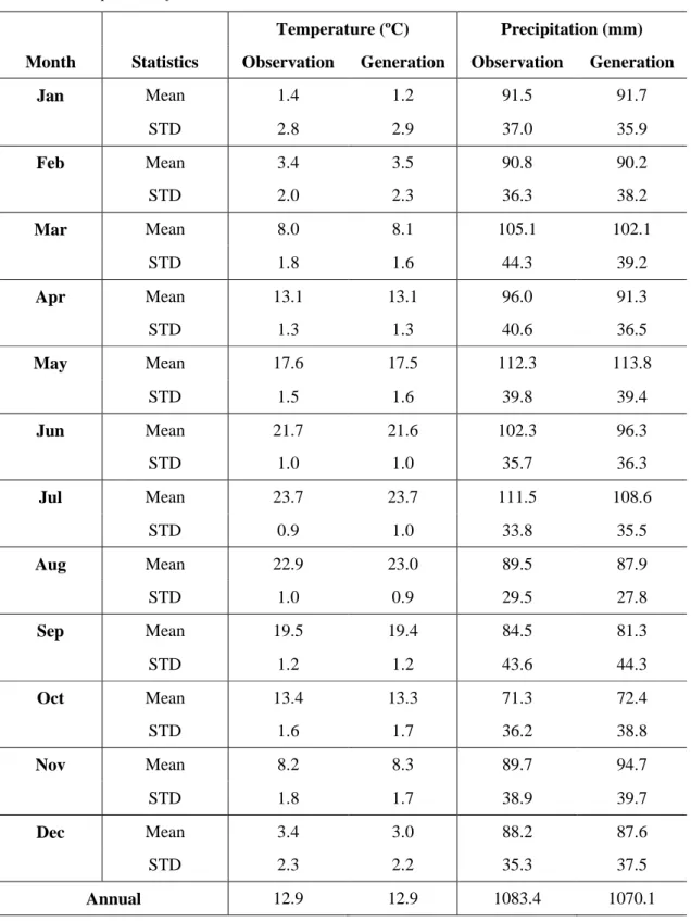
Lack of hydrologic information caused by short duration of observed climate data made the evaluation of long-term behavior of water resources system less reliable. To overcome this issue, this study generated a 200 year time-series of monthly T and P using the conditional generation method developed by Kim et al. (2008), which can preserve their inherent statistics of the observed data. This study assumed the generated monthly time-series of P and T as a base case climate condition (BASE) that represents current climate conditions of the study area.
The statistical characteristics of BASE were similar to those of the observed as shown in Table 3. Although not shown here, historical transition probability of P and T were also well preserved in the generated time-series.
3.1.2 Future Climate Scenarios
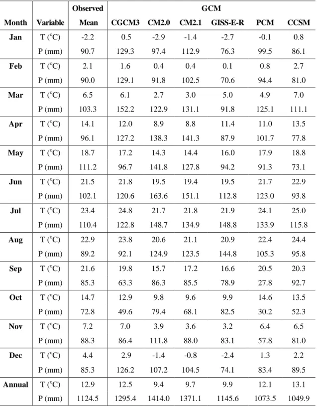
Weighting GCMs The selection of a certain GCM is difficult for a given region due to its uncertainty produced by assumptions and atmospheric processes specific to the GCM (Kim et al., 2008). The most appropriate method to assess the validity of GCM outputs is to compare with historical climate data for the same period (IPCC, 2000). The monthly P and T for the period of 1961 through 1990 from the baseline scenario (20C3M) of the six GCMs were compared to the observed P and T for the same period. The simulated P and T extracted from each GCM baseline scenario and the observed data were compared in Table 4.
Table 3. Comparison of Statistics between the Observed and Generated Time-Series Temperature (ºC) Precipitation (mm) Month Statistics Observation Generation Observation Generation
Jan Mean 1.4 1.2 91.5 91.7 STD 2.8 2.9 37.0 35.9 Feb Mean 3.4 3.5 90.8 90.2 STD 2.0 2.3 36.3 38.2 Mar Mean 8.0 8.1 105.1 102.1 STD 1.8 1.6 44.3 39.2 Apr Mean 13.1 13.1 96.0 91.3 STD 1.3 1.3 40.6 36.5 May Mean 17.6 17.5 112.3 113.8 STD 1.5 1.6 39.8 39.4 Jun Mean 21.7 21.6 102.3 96.3 STD 1.0 1.0 35.7 36.3 Jul Mean 23.7 23.7 111.5 108.6 STD 0.9 1.0 33.8 35.5 Aug Mean 22.9 23.0 89.5 87.9 STD 1.0 0.9 29.5 27.8 Sep Mean 19.5 19.4 84.5 81.3 STD 1.2 1.2 43.6 44.3 Oct Mean 13.4 13.3 71.3 72.4 STD 1.6 1.7 36.2 38.8 Nov Mean 8.2 8.3 89.7 94.7 STD 1.8 1.7 38.9 39.7 Dec Mean 3.4 3.0 88.2 87.6 STD 2.3 2.2 35.3 37.5 Annual 12.9 12.9 1083.4 1070.1
Table 4. Comparison of the Observed and GCM Simulated Climate Data for 1961 to 1990
Observed GCM
Month Variable Mean CGCM3 CM2.0 CM2.1 GISS-E-R PCM CCSM
Jan T (oC) -2.2 0.5 -2.9 -1.4 -2.7 -0.1 0.8 P (mm) 90.7 129.3 97.4 112.9 76.3 99.5 86.1 Feb T (oC) 2.1 1.6 0.4 0.4 0.1 0.8 2.7 P (mm) 90.0 129.1 91.8 102.5 70.6 94.4 81.0 Mar T (oC) 6.5 6.1 2.7 3.0 5.0 4.9 7.0 P (mm) 103.3 152.2 122.9 131.1 91.8 125.1 111.1 Apr T (oC) 14.1 12.0 8.9 8.8 11.4 11.0 13.5 P (mm) 96.1 127.2 138.3 141.3 87.9 101.7 77.8 May T (oC) 18.7 17.2 14.3 14.4 16.0 17.9 18.8 P (mm) 111.2 96.7 141.8 127.8 94.2 91.3 73.1 Jun T (oC) 21.5 21.8 19.5 19.4 19.5 21.7 22.9 P (mm) 102.1 120.6 163.6 151.1 112.8 123.0 93.8 Jul T (oC) 23.4 24.8 21.7 21.8 21.9 24.1 25.0 P (mm) 110.4 122.8 148.7 134.9 148.8 133.9 115.8 Aug T (oC) 22.9 23.8 20.6 21.1 20.9 22.4 24.4 P (mm) 89.2 92.1 124.9 123.5 144.8 105.3 95.8 Sep T (oC) 21.6 19.8 15.7 17.2 16.6 20.5 20.3 P (mm) 85.3 63.3 86.3 85.5 78.9 27.8 92.7 Oct T (oC) 14.7 12.9 9.8 9.6 9.9 14.6 13.5 P (mm) 72.8 49.6 79.4 68.1 82.5 30.2 52.3 Nov T (oC) 7.2 7.0 3.9 3.6 3.2 6.4 6.5 P (mm) 88.3 86.4 111.8 88.0 83.1 57.8 81.0 Dec T (oC) 4.4 2.9 -1.4 -0.8 -2.4 1.3 2.2 P (mm) 85.3 126.2 107.2 104.5 74.1 83.4 89.5 Annual T (oC) 12.9 12.5 9.4 9.7 9.9 12.1 13.1 P (mm) 1124.5 1295.4 1414.0 1371.1 1145.6 1073.5 1049.9
As presented in Table 4, the annual averages T of the GCM-simulated baseline range from 9.4°C (CM2.0) to 13.1°C (CCSM) while the observed annual T is 12.9°C. The GCM-simulated annual averages of P are 1295 mm (CGCM3), 1414 mm (CM2.0), 1371 mm (CM2.1), 1146 mm (GISS-E-R), 1074 mm (PCM), and 1050 mm (CCSM), while the observation is 1125 mm. The simulated monthly T data of CGCM3, PCM, and CCSM are relatively close to the observation, but CM2.0, CM2.1, and GISS-E-R underestimated monthly T over all seasons. The GISS-E-R, PCM and CCSM models simulate within 7% of the annual observed P value whereas the others estimated over 15%. The CGCM3, CM2.0, and CM2.1 models seasonally overestimate up to 60% compared to the observed annual P. Typical trends of the monthly mean P of the six GCMs generally follow the observations in spring, summer, and winter, but all six GCM underestimate the fall season. Although the GISS-E-R model is the closest to the observed annual P, this model is most biased to simulate the seasonal P.
The mean absolute error between each GCM-simulated baseline climate data and the observation was computed and inversely weighted to assign a weighting factor to each GCM. As presented in Table 5, CCSM shows the most reliable simulation in both precipitation (weight = 27.2%) and temperature (weight = 24.6%) on the study area because it managed to simulate both the total amount and the trend of monthly precipitation, and CM2.0 shows the lowest weights in both (weights = 12.9% and 8.7%). These weighting factors were multiplied to the corresponding GCMs outputs, and the results were summed to present an ensemble average of the six GCMs.
As a result, this study provided total 14 future climate conditions: seven future climate scenarios (six GCMs + a weighted scenario (WEIGHT)) under two different emissions scenarios (A2 and B1).
Table 5. Weighting Factors for Six GCMs GCM Country Weight (%) Precipitation Temperature CGCM3 Canada 12.7 23.9 CM2.0 U.S.A 12.9 8.7 CM2.1 U.S.A 14.6 9.2 GISS-E-R U.S.A 18.0 10.1 PCM U.S.A 14.7 23.4 CCSM U.S.A 27.2 24.6
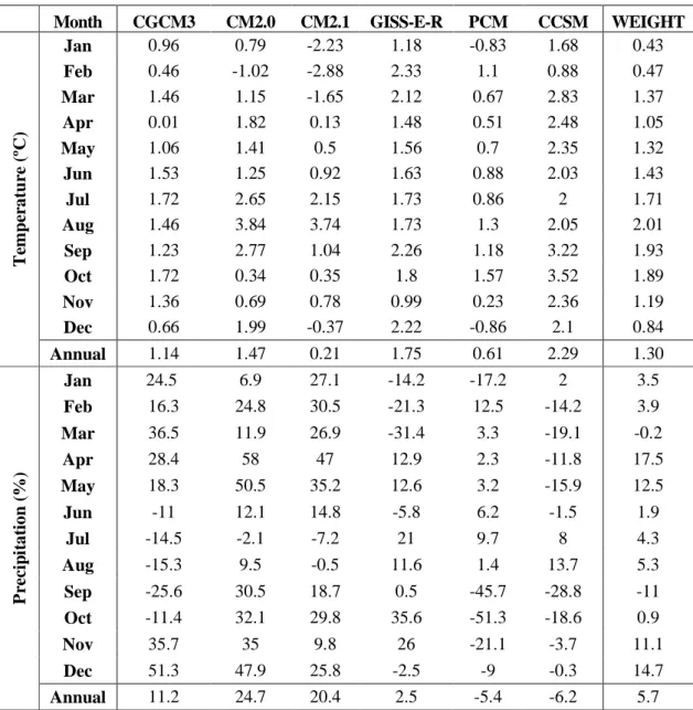
Future Climate Variables The changes of P and T of the six GCMs were extracted from their raw gridded outputs for the periods of 2030s, 2050s, and 2070s under two different emissions scenarios (A2 and B1). Tables 6 and 7 present the changes of P and T for the 2050s as a demonstration. The changes in those variables were used in perturbing the climate variables of BASE to represent the future climate conditions for the specific periods.
As summarized in the Table 6 and 7, the monthly means of T of the six GCMs and WEIGHT show a general increase with the higher increase in fall and the lower increase in winter, but the mean precipitation changes vary with months depending on the emissions scenarios. The monthly P of CGCM3 is expected to decrease to -25.6% in September and to increase up to 51.3% in December under A2, while B2 shows the range of -19.1% to 46.4% for the same months. P simulated by CM2.0 and CM2.1 shows the similar changes in pattern, as decreased in late summer and higher increased in spring and early summer. GISS-E-R uniquely projects droughts in winter and spring presenting as low as the -31.4% change of monthly P. PCM and CCSM generally underestimate the monthly P in both A2 and B1.
WEIGHT in both A2 and B1 shows the increased annual temperature with the higher rise in late summer and early fall and the increased annual precipitation with the higher rise in spring
and winter. However, P in fall shows the decreases of -11.0% and -16.2% in A2 and B1, respectively. The reduced P in fall could significantly affect the study area with a higher increase of T thus the higher evapotranspiration rate because the fall season of the study area usually experiences drought. In addition, the overall increases of the precipitation could influence the local floods.
Table 6. Changes of Climate Variables for the 2050s under the A2 Emission Scenario
Month CGCM3 CM2.0 CM2.1 GISS-E-R PCM CCSM WEIGHT
T em p er a tu re ( ºC ) Jan 0.96 0.79 -2.23 1.18 -0.83 1.68 0.43 Feb 0.46 -1.02 -2.88 2.33 1.1 0.88 0.47 Mar 1.46 1.15 -1.65 2.12 0.67 2.83 1.37 Apr 0.01 1.82 0.13 1.48 0.51 2.48 1.05 May 1.06 1.41 0.5 1.56 0.7 2.35 1.32 Jun 1.53 1.25 0.92 1.63 0.88 2.03 1.43 Jul 1.72 2.65 2.15 1.73 0.86 2 1.71 Aug 1.46 3.84 3.74 1.73 1.3 2.05 2.01 Sep 1.23 2.77 1.04 2.26 1.18 3.22 1.93 Oct 1.72 0.34 0.35 1.8 1.57 3.52 1.89 Nov 1.36 0.69 0.78 0.99 0.23 2.36 1.19 Dec 0.66 1.99 -0.37 2.22 -0.86 2.1 0.84 Annual 1.14 1.47 0.21 1.75 0.61 2.29 1.30 P re ci p it a ti o n ( % ) Jan 24.5 6.9 27.1 -14.2 -17.2 2 3.5 Feb 16.3 24.8 30.5 -21.3 12.5 -14.2 3.9 Mar 36.5 11.9 26.9 -31.4 3.3 -19.1 -0.2 Apr 28.4 58 47 12.9 2.3 -11.8 17.5 May 18.3 50.5 35.2 12.6 3.2 -15.9 12.5 Jun -11 12.1 14.8 -5.8 6.2 -1.5 1.9 Jul -14.5 -2.1 -7.2 21 9.7 8 4.3 Aug -15.3 9.5 -0.5 11.6 1.4 13.7 5.3 Sep -25.6 30.5 18.7 0.5 -45.7 -28.8 -11 Oct -11.4 32.1 29.8 35.6 -51.3 -18.6 0.9 Nov 35.7 35 9.8 26 -21.1 -3.7 11.1 Dec 51.3 47.9 25.8 -2.5 -9 -0.3 14.7 Annual 11.2 24.7 20.4 2.5 -5.4 -6.2 5.7
Table 7. Changes of Climate Variables for the 2050s under the B1 Emission Scenario
Month CGCM3 CM2.0 CM2.1 GISS-E-R PCM CCSM WEIGHT
T em p er a tu re ( ºC ) Jan 0.38 -0.01 -1.5 0.72 0.61 1.48 0.53 Feb 0.75 -1.16 -2.01 -0.49 0.51 1.88 0.43 Mar -0.17 0.71 -0.79 1.56 0.76 2.87 0.99 Apr 0.06 0.42 0.63 1.52 0.71 2.34 1.00 May 0.82 1.53 0.62 1.59 0.04 1.73 0.98 Jun 1.17 0.7 0.99 1.47 0.28 2.17 1.18 Jul 0.99 1.58 1.64 1.4 0.61 2.05 1.31 Aug 1.36 2.99 2.64 1.2 0.97 1.43 1.53 Sep 1.11 1.76 1.09 1.25 0.67 1.94 1.28 Oct 1.38 0.69 1.9 1.72 1.08 1.37 1.33 Nov 0.65 0.3 1.85 0.19 -0.16 2.17 0.87 Dec -0.17 -0.53 0.21 1.19 -0.95 1.94 0.31 Annual 0.69 0.75 0.61 1.11 0.43 1.95 0.98 P re ci p it a ti o n ( % ) Jan 24.2 5.6 5.2 -28.2 5.3 12.2 3.7 Feb 24.9 20.7 5.8 -23.8 11.3 -28.1 -3.5 Mar 13.2 24.9 7.5 -25.5 10.6 -17.4 -1.7 Apr 25.9 26.6 34.8 14.6 4.2 -27.7 7.6 May 11.7 56.9 10.3 8.5 9.1 -14.9 9.2 Jun -2 25.9 28.3 -3.4 16.3 -19.7 3.8 Jul -18.9 12.6 -14.9 19.8 -6.7 4.1 0.8 Aug -16.9 -15.6 -13.5 27.2 -7.5 12.8 1.2 Sep -19.1 -0.1 5.4 4.8 -53.9 -28 -16.2 Oct 4.4 14.1 15.7 16.3 -32.5 -29.1 -5 Nov 30.9 37.1 17.2 2.4 -20.9 -0.6 8.5 Dec 46.4 11.5 27.2 -18.1 -11.7 6.1 8.1 Annual 9.4 18.4 10 -0.4 -3.7 -9.7 1.9
3.2 Runoff Generation
Runoff is the output of the water balance model using climate variables as inputs. After calibrating the model parameters, climate variables generated for different climate conditions were used to simulate various runoff sets (i.e., BASE, six GCMs and WEIGHT for the 2030s, 2050s, and 2070s under A2 and B1 emissions scenarios).
3.2.1 Calibration and Validation
The water balance model was calibrated and validated using observed climate variables and runoff from 1970 to 2005, and the results are shown in Figure 7. This study divided the observation data into two periods, 1970 to 1999 and 2000 to 2005 for calibration and validation, respectively.
Figure 7. Calibration and Validation of the Water Balance Model.
The calibration results suggest a good agreement between the observed and simulated runoff by showing a NS coefficient of 0.74 and coefficient of determination (R2) of 0.75. The model is then validated for the last six years using the calibrated model parameters, resulting an acceptable performance with NS = 0.68 and R2 = 0.71 (Figure 7).
0 20 40 60 80 100 120 140 160 180 200 1 25 49 73 97 121 145 169 193 217 241 265 289 313 337 361 385 409 R u n o ff ( m m ) Months (1970-2005) Observed Modeled Validation R2 = 0.71 NS = 0.68 Calibration R2 = 0.75 NS = 0.74
3.2.2 Runoff Generation for Climate Scenarios
Climate variables from the 43 sets of climate condition (one BASE + three periods*two emissions scenarios*(six GCMs + one WEIGHT)) were used as inputs to the calibrated water balance model to construct runoff time-series. The overall trend of seasonal runoff changes using the WEIGHT scenarios show that runoff increases in spring, summer, and winter, and decreases in fall, compared to BASE (Figure 8). These results follow the pattern of precipitation changes of the WEIGHT scenarios (see Tables 6 and 7).
Figure 8. Percent Changes of Runoff for Different Emissions Scenarios and Time Periods using WEIGHT.
In Figure 8, the A2 scenario shows more increased runoff (annually 8.0%) and higher variation than the B1 scenario (annually 5.7%). This trend generally follows the changes of climate variables for the emissions scenario of A2 and B1. In the A2 scenario, the biggest increase of the total annual runoff occurs in the 2050s rather than in the 2070s because the increased temperature in the 2070s may increase evapotranspiration than the precipitation increase, whereas the largest increase in the B2 scenario occurs in the 2070s.
In detail of the A2 scenario, the range of changes in monthly runoff is from -17% to 23% over time with the higher increases in April, May, and December and the decreases in the fall seasons (September and October). The highest increase (23%) of runoff is simulated in the 2050s under A2, while the largest decrease (-17%) in the 2070s. The range of month runoff by the B1 scenario is from -24 % to 17%, and the seasons showing the most difference are same as in the A2 scenario. The significant changes of the runoff are the increases in winter through summer and the decreases in fall (23% on May in the 2050s under A2 and -24% on October in the 2070s under B1).
As shown in the climate and hydrology of the study area, the flood usually occurs in the winter through early spring by prolonged heavy precipitation and low evapotranspiration and in the summer by heavy downpours from thunderstorms. The drought frequently happens in fall by low precipitation and high evapotranspiration (NOAA, 2002). Thus, based on the GCM-simulated future climate conditions, such changes of the runoff pattern would drive the frequency and intensity of flood and drought to increase in the study area, and the changes of the frequency and intensity could influence the existing water resources management plan.
This study further analyzed the long-term hydrologic regimes over the Norris Dam area in terms of flow duration and evaluated the future performance of dam operation (mainly hydropower generation) using the generated runoff sets as inflows to Norris Dam.
3.3 Hydrologic Regimes and Performance of Dam Operation
For more reliable analysis of flow duration and dam operation, this study generated 200-year time-series of climate variables for different climate conditions and the runoff was simulated as well according to all climate conditions.
3.3.1 Changes of Flow Duration
Many aspects of hydrologic regimes of a watershed can be addressed through flow duration curves driven from long-term runoff observation. This study estimated monthly flow duration curves for different climate conditions and displayed for BASE, maximum and minimum from six GCMs, and WEIGHT to provide more comprehensive overviews (Figure 9).
The flow duration curves show an upward tendency (i.e., the weighted runoff plotted above that of BASE) (Figure 9). The differences between the weighted and baseline runoffs tend to increase in the higher runoff (or lower exceeding probability).
As shown in Table 8, due to the increased runoff, the Q10 and Q50 of WEIGHT in both
scenarios gradually increase overall period, but the Q90 slightly increases with an irregular trend
in time and even decreases in the 2030s of the B1 scenario. The highest increase of runoff occurs in the 2050s of the A2 scenario while, in the B1 scenario, the highest runoff is in the 2070s. A significant issue is that the percent change of the Q90 decreases from 10.4% in the 2050s to 0.5%
in the 2070s in WEIGHT of the A2 scenario mainly due to the highest increase in temperature in the 2070s. The decreased Q90 means that the probability of drought occurrence would increase
even though the Q50 in the 2070s is decreased to 5.6% from 10.1% in the 2050s. Also, the
probability of a flood would increase over time because the Q10 in the A2 scenario would increase
up to 12% in WEIGHT. The increased Q10 and decreased Q90 in the 2070s imply that the climate
variation of the study area will be extremely severe.
Moreover, because the climate models include uncertainty and variability, the maximum and minimum runoff should be meaningful to extreme future climate conditions. When the maxima and minima are considered as the range of the predicted future runoff, the Q10, Q50, and
Q90 are ranged up to 43%, 48%, and 93% in the 2070s of the A2 scenario, respectively (the lower
Figure 9. Comparison of Flow Duration Curves for Different Emission Scenarios and Time Periods.
Maximum Minimum
Table 8. Average Percent Changes of Flow Statistics for Two Emissions Scenarios A2 Scenario (%) B1 Scenario (%) Case Period Q10 Q50 Q90 Q10 Q50 Q90 WEIGHT 2030s 2.3 1.7 3.4 4.5 2.6 -0.3 2050s 11.7 10.1 10.4 5.9 4.9 2.8 2070s 12.4 5.6 0.5 10 4.9 1.7 Max 2030s 20.3 22.7 48.1 23.8 22.4 42 2050s 31.9 28.6 58.9 28.1 28.4 53 2070s 36.4 29.2 40.4 25.5 21.8 41 Min 2030s -13 -17.8 -36.9 -11.9 -16.4 -35.1 2050s -6.4 -7.8 -28.2 -11.1 -16.2 -39.2 2070s -6.1 -18.7 -52.2 -7.2 -13.3 -38.3
Q10, Q50, and Q90 represent 10%, 50%, and 90% flows in flow duration curves, respectively.
3.3.2 Performance Evaluation of Dam Operation
A hydrologic routing method based on water mass balance was used to generate hypothetical dam operation data (outflow) for all climate conditions suggested in this study. Because there was no published dam operation rule, this study assumed the observed mean monthly outflow to be the required outflow of the month while keeping flood guidelines (Figure 4).
This study evaluated the performance of future dam operations using an evaluation criterion, i.e., the observed mean monthly outflow. The 200-year outflow sets, which were routed from the 200-year inflow time-series, were used to calculate RRV as performance indices. The increases of reliability and resilience indicate a more robust dam operation; in contrast, the decrease in vulnerability indicates less failure of dam operation. The changes of RRV values for different emissions scenarios compared to those of BASE are summarized in Table 9 using WEIGHT as well as minimum and maximum from the six GCMs results.
The results in Table 9 suggest that the reliability and resilience for the outflow of WEIGHT entirely increase at least 2% to 8% and 5% to 22%, respectively, and the vulnerability
of time and volume is alleviated in most future climate conditions up to one month and -99%, respectively.
Table 9. Changes of Reliability, Resilience, and Vulnerability of Future Dam Operation using WEIGHT
Condition REL RES VULT VULV
BASE 0.78 0.76 12 months -1782 MCM A2 WEIGHT 2030s 0.79 2% 0.80 5% 13 8% -1908 7% 2050s 0.84 8% 0.96 26% 3 -75% -480 -73% 2070s 0.83 6% 0.93 22% 5 -58% -764 -57% Max 2030s 0.87 12% 1.00 31% 18 50% -3204 80% 2050s 0.88 14% 1.00 31% 16 33% -2996 68% 2070s 0.88 13% 1.00 31% 16 33% -2850 60% Min 2030s 0.59 -24% 0.45 -41% 2 -83% -28 -98% 2050s 0.68 -12% 0.59 -23% 1 -92% -9 -99% 2070s 0.63 -19% 0.51 -33% 1 -92% -9 -99% B1 WEIGHT 2030s 0.80 3% 0.83 9% 13 8% -1674 -6% 2050s 0.81 5% 0.87 14% 7 -42% -1111 -38% 2070s 0.82 6% 0.92 21% 5 -58% -725 -59% Max 2030s 0.87 12% 1.00 31% 17 42% -3002 68% 2050s 0.88 13% 1.00 31% 18 50% -2978 67% 2070s 0.87 12% 1.00 31% 15 25% -2906 63% Min 2030s 0.60 -23% 0.47 -38% 1 -92% -9 -99% 2050s 0.61 -22% 0.48 -37% 1 -92% -9 -99% 2070s 0.66 -15% 0.55 -28% 1 -92% -9 -99%
REL = reliability, RES = resilience, and VULT and VULV = vulnerability in terms of time and volume,
respectively.
In summary, from the assessment of the RRV indices and the flow duration curve, the hydrologic robustness of water quantity is expected to improve over time in both emissions scenarios. However, it should be noted that, based on the changes in minimum and maximum of RRV, individual GCMs results show deteriorated operational performance for the future. This result should be interpreted as an uncertainty of the future climate conditions simulated from
GCMs. Although the overall increase of runoff is beneficial to water resources management for hydropower generation and water supply, the risks of flood and water shortage are still present in the future depending on the seasons and emissions scenarios. Also, due to the sediment accumulation at the bottom of Norris Lake, its capacity for flood control will be gradually diminished and the flood risk can be increased in the future even with the similar runoff to the current condition.
3.4 Water Quality
Few research data of water quality analysis have been identified in the study area mainly due to the limited monitoring data of water quality. Therefore, basic water quality indices (stream temperature and DO concentration) were analyzed using the data sets obtained from EPA STORET and USGS. The observed data showed that air temperature increased in late summer through fall, in which a drought period usually starts and the DO concentration generally lowers.
3.4.1 Steam Temperature
Stream temperature of the study area indicates that there is a similar trend to air temperature (Figure 10), implying a regression method applicable to build a stream temperature prediction model.
The relationship between air and stream temperature are presented in Figure 11. Since there was no significant nonlinear trend in the scatter plot, this study corrleated the stream temperate data with air temperature using a linear regression model. The regression coefficents were estimated using the method of least squares resulting the coefficient of determination value 0.96. This relationship strongly indicates the future changes of stream temprature will be mainly dominated by air temperature.
Figure 11. Relationship between Air Temperature and Stream Temperature measured at Cleveland, VA.
From the estimated regression model, this study projected the future stream temperature change over different time periods using the air temperature data of WEIGHT under two emissions scenarios. Depending on the emissions scenarios, the changes of stream temperature of the study area range from 0.1 to 3.0oC by the 2070s (Figure12). The high increase in stream temperature during late summer and fall seasons needs particular attention for potential negative environmental issues.
Figure 12. Mean Changes of Stream Temperature Projected for Different Emissions Scenarios and Time Periods using WEIGHT.
3.4.2 DO Concentration
A prediction model for DO concentration as a function of stream temperature can also be driven by a linear regression since any significant nonlinear trend was not detected. The regression coefficients were estimated through the method of least squares (R2 = 0.77) (Figure 13). Considering the insufficient number of data, the regression model was acceptable in suggesting the changes of future DO concentration using the projected stream temperature.
Figure 13. Relationship between Stream Temperature and DO Concentrations obtained from EPA STORET.
DO concentrations were computed using the regression model (Eq. in Figure 13) using the stream temperature generated earlier. The monthly mean DO concentrations are presented for two emissions scenarios and different time periods in the future (Figure 14). The A2 scenario shows a greater dropdown of DO concentration with time during the summer season than the B2 scenario. This tendency is similar to the projection of air temperature for two emission scenarios. Considering the General Water Quality Criteria 1200-4-3 of Tennessee Department of Environment and Conservation (TDEC, 2008), in which the Clinch River is designated as trout water with a DO concentration regulatory higher than 8.0 mg/L, aquatic ecology including trout that relies on DO concentration may be impacted during the summer season (Silver et al., 1963).
Figure 14. Monthly Mean DO Concentration Projected for Different Emissions Scenarios and Time Periods using WEIGHT.
Chapter 4
Summary, Conclusions and Recommendations
This study assessed the potential impacts of climate change on hydrology, the water resources system, and the water quality of Norris Lake including the Upper Clinch and Powell River basins. The future climate data were projected from the six GCMs forced by two emissions scenarios (A2 and B1). The runoff hydrographs of the study area were simulated using the projected future climate data and a water balance model.
The generated runoff hydrographs under different climate conditions were used to evaluate the changes of hydrologic regimes and performance of dam operation. For this purpose, flow duration curves and performance evaluation indices were computed and compared with those of the base case scenario. Simple water quality prediction models were driven by observed stream temperature, air temperature, and DO concentration.
Key findings of the study can be summarized as follows:
1. In analyzing the baseline scenario of the six GCMs, CCSM is most reliable to simulate the current climate conditions of the study area (i.e., precipitation and temperature observed from 1961 to 1990), and CM2.0 shows the lowest credibility to simulate these climate variables. The weighted GCMs scenario for the 2070s shows the slightly increased drought occurrence in fall due to the higher increased temperature compared to other seasons.
2. The water balance model was reasonably calibrated and validated with the Nash- Sutcliffe coefficient and R2 over 0.70. The calibrated model parameters were then used to generate the future runoff time-series. The significant changes are the increased runoff
from winter through summer and the decreases in fall (about 23% in May and -24% in October). These changes of the runoff pattern may affect the frequency and intensity of the floods and droughts in the study area.
3. The overall robustness in water quantity of the study area is expected to improve over time in the both emissions scenarios based on the uplifted flow duration curves of the weighted GCMs scenario compared to those of the base case runoff scenario. The probability of the flood and drought also is likely to increase due to the runoff variation with uncertainty of the future climate changes. The results of the RRV analysis for the future dam outflow suggest that the reliability, resilience and vulnerability of time and volume for the hydropower generation and water supply are expected to be improved mainly due to the overall increased streamflow compared to the current conditions. However, this increased streamflow would affect the flood risk of Norris Dam with accumulated sedimentation over time.
4. The linear regression models of the monthly stream temperature and DO concentration were established with the remarkable coeffieints of determination. As a result, it is expected that the future stream temperature would increase up to 3ºC in the 2070s and consequently the study area can suffer the decreases of DO concentration in summer and fall.
In conclusion, with the presence of high uncertainty in GCM outputs, the wetter and warmer climatologic changes generally would increase the runoff and hydropower generation of the study area. However, the hydrologic severity of flood and drought could also increase because the expected range of the future runoff remains in high variation. Moreover, due to the warmer