Exact solutions for cluster growth kinetics with evolving size and shape profiles

Exact solutions for cluster-growth kinetics with

evolving size and shape profiles

Jonathan AD Wattis

Theoretical Mechanics, School of Mathematical Sciences, University of Nottingham, University Park, Nottingham, NG7 2RD, UK.

E-mail: [email protected]

Abstract. In this paper we construct a model for the simultaneous compaction by which clusters are restructured, and growth of clusters by pairwise coagulation. The model has the form of a multicomponent aggregation problem in which the components are cluster mass and cluster diameter. Following suitable approximations, exact explicit solutions are derived which may be useful for the verification of simulations of such systems. Numerical simulations are presented to illustrate typical behaviour and to show the accuracy of approximations made in deriving the model. The solutions are then simplified using asymptotic techniques to show the relevant timescales of the kinetic processes and elucidate the shape of the cluster distribution functions at large times.

PACS numbers: 64.60.Ht 82.60.Nh 05.70.Fh

Submitted to: J. Phys. A: Math. Gen.

1. Introduction

It would be useful to have models of nucleation which describe the differences in both size and shape of growing clusters and yet are simple enough to be solvable analytically. Current exactly solvable models of coagulation only describe cluster masses. As well as elucidating the kinetics of aggregation and compaction, models involving size and shape would be useful in the testing of numerical simulations of systems such as those used by Xiong et al [24, 25]. An alternative approach which takes explicit account of the separately evolving size and shape of a typical cluster is given by Schild et al

Pratsinis [20] where such a one-component model is analysed in an attempt to find the self-preserving shape of cluster-size distribution.

Ideally the results described below should be calibrated against experimental data, or data from computer simulations, for example the work on sintering carried out by Akhter et al [2], where computer simulations are compared to experimental data. However, we would not expect exceptionally good agreement from the models solved in this paper, since these have no size or shape dependence in the aggregation kernels. More realistic kernels could be used, and then it would be interesting to compare numerical solutions of such models against experimental data and other simulation techniques. Kostoglou et al [13, 14] and di Stasio et al [17] have also worked on modelling simultaneous coagulation and restructuring of cluster-shape. Another area where two-component aggregation problems naturally arise is that of charged clusters [19, 4, 3], where clusters are characterised independently by size and charge.

Other work on multicomponent coagulation problems includes that of Elvingson & Wall [11, 21] who developed a two-component version of the Becker-D¨oring equations to model the formation of mixed micelles, these are clusters formed from two-species of surfactant molecule. A similar model has been analysed by Wu [23]. Multi-component Becker-D¨oring systems have been used in several models of the kinetics of vesicle formation [9, 6, 7]. However, the situations under consideration in this paper require Smoluchowski [16] aggregation rather than the restricted stepwise growth of Becker-D¨oring models. An unusual multi-component coagulation which includes Smoluchowski-type aggregation arises in the modelling of river-flow [8], where to make progress on the analysis the system is again approximated by a single-component problem. In a few special cases of multicomponent Smoluchowski aggregation, exact solutions are available [22], and the solution constructed in this paper relies on the ideas and methodology presented there.

In Section 2 we derive a multicomponent model of simultaneous coagulation and compaction which is of Smoluchowski type. This model is solved in Section 3 by means of generating function techniques. A numerical solution is also performed to allow us to analyse some of the errors made in the modelling assumptions. The large-size and large-time asymptotics of the exact solution is carried out in Section 4 – this allows some simplification of expressions. Finally a discussion of the results is presented in Section 5.

2. Model of simultaneous coagulation and compaction

2.1. Formulation of model

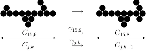
Cj,k

C15,9

-Cj,k−1

C15,8 −→

−→ −→

γ15,9 γj,k

yyyyyyyyyy y

yy y y

yyyyyyyyy y

yy y y

y

Figure 1. Illustration of compaction.

We then allow two processes to act on the distribution of cluster sizes: a restructuring of the cluster which transforms a fractal aggregate to make it more compact. This occurs through some geometric rearrangement of the cluster’s constituent parts so as to reduce its maximum diameter as illustrated in Figure 1. To each compacting event we assign a transition rateγj,k. Once a cluster is maximally compact

(i.e. its maximum diameter has reached some minimum) this process will be assumed to have no further influence on a cluster. If we follow the spherical liquid drop model of a cluster, then the minimum diameter for a cluster composed ofj monomers iskc(j)

such that 4 3π(

1 2kc(j))

3 _{=j/σ, where σ is the density of a monomer (sincej is a measure} of mass, j/σ is a volume). Thus kc(j) = (6j/πσ)1/3; if we work in units in which

the monomer has unit diameter, we find σ = 6/π; and hence kc(j) = j1/3. In other

applications, where clusters may preferentially form rod-like or disc-like aggregates, some other functional form of kc(j) may be more appropriate. Whilst we are interested

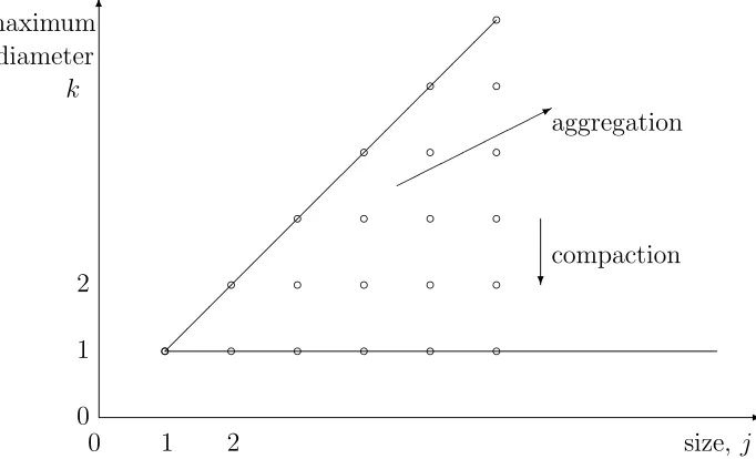
in the full range of cluster sizes 1 _≤ j < _∞, the range of maximum diameters k is restricted tokc(j)≤k≤j. This region of (j, k) space is illustrated in Figure 2.

-6

size, j maximum

diameter

k upper limit, k=j

linear approx to the lower limit k=kc(j), namely k = 1 +ε(j₋1)

lower limit, kc(j) = j1/3,

for example

A

Figure 2. Illustration of region of size (mass, j) and shape (maximum diameter,

k) parameter space which correspond to physically relevant clusters in the model of Section 2.1. The large letter ‘A’ denotes the admissible region.

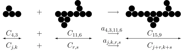
Clearly, the masses must simply sum, but clusters may combine in any orientation, so the maximum diameter of the aggregate maybe less than the sum of the maximum diameters of the initial clusters. Formally, we have

Cj,k+Cr,s→Cj+r,q, (2.1)

with q potentially taking any value from max_{k, s_} to k +s. In a mean field model, we should form some weighted average over all possible configurations. However, since we have a mechanism to reduce the cluster’s maximum diameter, we take the ‘worst’ case scenario of the greatest possible value of q, and allow the restructuring mechanism (Figure 1) to spread the resulting distribution over a range of diameters smaller than k + s. This mechanism is illustrated in Figure 3. Magnetic or electrically charged particles tend to form extremely elongated structures during growth by coagulation, see for example Kammleret al [12].

yyy y

C4,3

Cj,k

+

+

+

yyyyyy y y

yy y

C11,6

Cr,s

−→

−→ −→ aj,k,r,s a4,3,11,6

yyyyyyyyy y y

yy y y

C15,9

Cj+r,k+s

Figure 3. Illustration of aggregation of clusters of arbitrary sizes (r and j) and arbitrary shapes, this being described by each cluster’s maximum diameter (sandk).

Taking the two mechanisms illustrated in Figures 1 and 3 and applying the law of mass action to derive equations for the concentrations cj,k(t), we obtain

dcj,j

dt =Fj,j−Lj,j−γj,jcj,j, dcj,k

dt =Fj,k−Lj,k+γj,k+1cj,k+1−γj,kcj,k, (kc(j) + 1≤k < j) dcj,k

dt =Fj,k−Lj,k+γj,k+1cj,k+1, (kc(j)≤k < kc+ 1) (2.2) whereFj,k andLj,k are the rates of formation and loss of clustersCj,k through the usual

aggregation and fragmentation processes, that is

Fj,k = 1₂ j−1

X

r=1

k−1

X

k=1

ar,s,j−r,k−scr,scj−r,k−s, (2.3)

Lj,k =

∞

X

r=1

∞

X

s=1

ar,s,j,kcr,scj,k. (2.4)

2.2. Integrable model of coagulation and compaction

aggregation rate to solve are typically size-independent, thus we assume ar,s,j,k =a. In

place of the lower limitk =kc(j), we first approximatekc(j) by 1 +ε(j−1) withεsmall;

however, such models are in general still insoluble; to obtain an integrable system we take the limiting case and put ε= 0. This is equivalent to definingkc(j) = 1. In section

3.3 we solve the systems numerically and analyse the differences between systems with kc(j) = 1 and kc(j) = j1/3.

For the compaction rateγj,kwe assumeγj,k =γ(k−1) for some constantγ, since this

automatically becomes zero on the linek = 1, simplifying the mathematical formulation of the problem. Physically, it also has the advantage of assigning a high rate of diameter reduction to very ‘wispy’ aggregates (whose maximum diameter is close to their mass), and low rates of diameter reduction to clusters which are almost maximally compact. Thus as well as being mathematically convenient, we believe this to have good physical justification. For simplicity we do not include any size-dependence (j) in γj,k: the

rate at which the maximum diameter reduces depends only on the maximum diameter. Combining these assumptions for γj,k and aj,k,r,s, we obtain

˙ cj,k = 1₂

j−1

X

r=1

k−1

X

s=1

acr,scj−r,k−s− ∞

X

r=1

∞

X

s=1

acr,scj,k+

+γkcj,k+1−γ(k−1)cj,k, (2.5)

note that on the line k = 1, which represents the maximally compact clusters, the last term automatically vanishes, since no further compaction of these clusters can occur. The approximation of kc(j) by unity increases the region of (j, k) space accessible to

the model, as illustrated in Figure 4. Also, note that provided that cj,k(t) = 0 for k > j, is satisfied att= 0 then this condition is satisfied by the distribution at all later times. Thus we need to make no explicit specification of the condition k _≤ j in (2.5), or write out a special equation valid onk =j, since cj,j+1 = 0 automatically causes the penultimate term of (2.5) to vanish on k = j + 1. At t = 0, we assume the system is completely in monomeric form, that is, the initial data is cj,k = 0, for all j, k with the

exception ofc1,1 =%.

3. Solution of model

We will aim to solve the system using the generating function approach of Davies et al

[10], hence we introduce transform variables x,y and define

C(x, y, t) =

∞

X

j=1

∞

X

k=1

cj,k(t)e

−jx−ky

, (3.1)

and we also make use of an alternative generating function

G(x, y, t) =

∞

X

j=1

∞

X

k=1

cj,k(t)e

−(j−1)x−(k−1)y

, (3.2)

which is related to C(x, y, t) by G(x, y, t) = C(x, y, t)ex+y_{. Associated with these}

-6

size, j maximum

diameter k

bb b b

b b b

b b b b

b b b b b

b b b b b b

0 1 2

0 1

2 ?

compaction

*aggregation

Figure 4. Illustration of region of size (mass, j) and shape (maximum diameter, k) parameter space included in our explicitly solvable model system of Section 2.2. This corresponds to the caseε= 0 of the linear approximation to the lower limit illustrated in Figure 2.

system

C0(t) =G0(t) =C(0,0, t) =G(0,0, t). (3.3) The initial conditions for C are C(x, y,0) = %e−x−y

, whilst for G they take on the simpler form of G(x, y,0) =%; both of these imply C0(0) =G0(0) =%.

The equation for the generating function C(x, y, t) is ∂C

∂t = 1 2aC

2

−aC0C−γ(ey−1) C+ ∂C

∂y

!

. (3.4)

The associated equation for C0(t) is ˙C0 = −1₂aC02 which, when the initial condition C0(0) =% is imposed, has the solution

C0(t) =G0(t) = 2%

2 +a%t. (3.5)

Substituting C=Ge−x−y

into (3.4) we obtain ∂G

∂t +γ(e y

−1)∂G ∂y =

1 2aG

2_e−x−y

− 2%aG

2 +a%t. (3.6)

Solving by characteristics, with initial data on s = 0 parameterised by ξ, η of t = 0, x=ξ, y=η, G=% gives

t_≡s, x_≡ξ, 1₋e−y

= eγs(1₋e−η

), (3.7)

and

G = 4%

(2 +a%s)2_{K(ξ, η, s)}, (3.8) K(ξ, η, s) = 1 + e−ξ−η

+ 2e

−ξ

(1₋eγs_(1−e−η

))

+2γe

−2γ/a%

e−ξ

(1₋e−η

) a%

(

E1 − 2γ a%

!

−E1 − γ

a%(2 +a%s)

!)

.

Expanding G(x, y, t) as a power series in both e−x

and e−y

, we find the full explicit solution for each individual concentration

cj,k(t) =

4% (2+a%t)2

k j! j k! (j₋k)!

1₋e−γt

−E(t)j−k _E(t)+e−γt

− 2 2+a%t

!k−1

,

(3.10)

where

E(t) = 2γ a%e

−γt−2γ/a%

"

E1 − 2γ a%

!

−E1 − γ

a%(2 +a%t)

!#

. (3.11)

This is the exact explicit solution of the problem originally posed in (2.5), with initial data of cj,k = 0 for all j, k except for c1,1 =%. Although our aim was to construct such a solution, and it will be useful for verifying numerical solutions of such problems, it is not clear exactly the what behaviour is described by this function. Hence in the next section we will form approximations of it to show the kinetic phenomena it describes.

3.1. Analysis of moments

Using the generating function (3.8), we now find properties of the distribution, such as the behaviour of the first few moments. We define the joint moments by

Mp,q(t) =

∞ X j=1 ∞ X k=1

jpkqcj,k(t). (3.12)

The number of clusters is given byM0,0 =G(0,0, t); however, higher moments are given by more complex formulae. Since C =e−x−y

G=P∞

j=1

P∞

k=1cj,ke−jx−ky, we have Mp,q(t) =

(

−_∂x∂

!p

−_∂y∂

!q e−x−y

G(x, y, t))

(x,y)=(0,0)

, (3.13)

for exampleM0,1 =G(0,0, t)−Gx(0,0, t) andM2,0 =Gxx(0,0, t)−2Gx(0,0, t)+G(0,0, t).

In particular, we have

M0,0 = 2%

2 +a%t, M1,0 =%, M0,1 =%(E(t) + e

−γt

), (3.14)

M2,0 =%(1 +a%t), M0,2 =%

h

(3 +a%t)(e−γt

+_E(t))₋2i, (3.15) M1,1 =%(1−2(E(t) + e

−γt

) + (_E(t) + e−γt

)2(2 +a%t)), (3.16) where we have defined the time-dependent quantity _E(t) by (3.11).

From the moments (3.14)–(3.16), it is possible to derive quantities of macroscopic interest. For example, the average cluster size, J, can be derived in several ways:

J1 = M1,0 M0,0

= 1 +1₂a%t, J2 = M2,0 M1,0

= 1 +a%t, (3.17)

J3 = M1,1 M0,1

= (2 +a%t)(_E(t) + e−γt

)₋2 + 1

(_E(t) + e−γt

In systems which do not undergo any sort of gelation behaviour, all these definitions should give rise to broadly the same kinetic behaviour. Note that J1 and J2 are independent ofγ, as one would expect since compaction does not alter cluster mass, and neither does it affect the subsequent rate of cluster coagulation. However, J3 depends onγ –this definition of average cluster size showing some influence of the restructuring history of clusters. For a wide range of parameters γ, a% and most times t, the value of J3 lies betweenJ1 andJ2: at small timesJ3 is close to J2, at larger times,J3 approaches J1. For small γ/a%the crossover of J3 fromJ2 toJ1 occurs at large times, and for large γ/a% the crossover occurs at small times.

In a similar manner to (3.17)–(3.18), the average cluster diameter,K, can be defined by any of

K1 = M0,1 M0,0

= (1 +1₂a%t)(_E(t) + e−γt

), (3.19)

K2 = M0,2 M0,1

= 3+a%t₋ 2

E(t)+e−γt, (3.20)

K3 = M1,1 M1,0

= 1₋2(_E(t) + e−γt

) + (_E(t) + e−γt

)2(2 +a%t). (3.21)

3.2. Fractal dimension

In our definitions, the volume of a cluster Cj,k scales with its aggregation number, thus V _∼ j, and the diameter scales with L _∼ k. For fractal clusters, the dimension D is defined by V = LD _{or D = log(V)/log(L). Using the definitions (3.17)–(3.21), nine}

different fractal dimensions can be constructed

Dp,q =

logJp

logKq

. (3.22)

At small times, we expect the growing clusters to be linear in geometry, thus to have dimension close to unity. However, of the nine definitions, two give rise to dimensions of two (D2,1,D3,1) and two more to dimensions of one half (D1,2, D1,3).

This leaves five definitions of dimensions, which are plotted in Figure 5. From this we see that two give quite low estimates, and one of these gives dimensions below unity, which we discount as unphysical In the left-hand graph, where γ = 0.01, we expect compaction to occur on the timescale t = _O(1/γ), thus the second lowest curve also gives a compaction timescale which is unexpectedly long. The upper three curves all give qualitatively similar results. A similar outcome is observed when γ = 1, suggesting that the definitionsD1,1,D2,2and D3,2 should be preferred over the others. The upper curves in Figure 5 exaggerate the compaction effect, as fractal dimensions greater than three are only possible because of the approximation we make when relaxing the constraint k _≥(6j/πσ)1/3 _{tok ≥1.}

100 3

2

0 0 1.5

500 300 t 400

200 2.5

0.5 1

3

2

0 2.5

5 2

1 0.5

1

3 1.5

4 t 0

Figure 5. Plots of fractal dimension against time for the parameter values a = 1,

%= 1; on the leftγ= 0.01, and on the rightγ= 1. Starting with the uppermost, the curves in the left hand plot representD22, D32, D11,D23 andD33. and those in the

right-hand plot representD2,2,D1,1,D3,2, D2,3,D3,3.

of the whole population is thus given by an average of the form

f

Dp,q,r,s=

∞

X

j=1

∞

X

k=1

jp_kq_(logj)r+1_(logk)s−1

cj,k(t)

∞

X

j=1

∞

X

k=1

jpkq(log(j)r(logk)scj,k(t)

, (3.23)

for some constants p, q, r, s. Unfortunately formulae such as (3.23) cannot be explicitly be evaluated given the form of our solution (3.10).

3.3. Numerical solution

In Figure 5 we observe several of the curves rising rapidly to dimensions above three. The reason for this is that in Section 2.2, when deriving a set of equations which are explicitly integrable, we replaced kc = j1/3 by kc = 1. This significantly alters the

calculation of the dimension of the more compact clusters. To assess the implications of this approximation, we have used Matlab to solve the system of ordinary differential equations (2.2) with γj,k =γ(k−kc(j)) and ar,s,j,k =a in both the cases kc(j) = 1 (the

integrable case) andkc(j) = j1/3. The outputs were used to calculate the average cluster

sizes Jp and diameters Kq and the fractal dimensions Dp,q (1≤p, q ≤3). A sample of

0

10

20

30

5

10

15

time, t

J2, K2

0

10

20

30

1

1.5

2

2.5

3

time, t

dimension

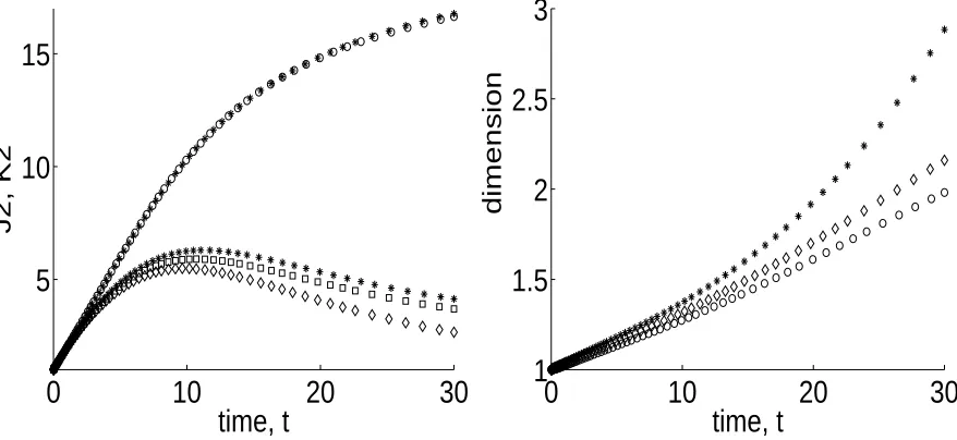
Figure 6. Plots of average cluster size, maximum diameter and fractal dimension against time for the parameter values a = 1, % = 1, γ = 0.1, for a system size of

j, k≤N= 30.

Left: the top three lines of data points correspond to calculations of the average cluster size J2 = M2,0/M1,0 and are almost superimposed: ‘+’ denotes the exact

solution (kc = 1), circles denote the numerical solution of the case with kc = j1/3,

and crosses represent points from thekc= 1 calculation rescaled by (3.24). The lower

three data sets correspond to calculations ofK2=M0,2/M0,1, here ‘*’ represents the

numerical solution of the system with kc = j1/3, the diamonds correspond to the

exactly solvable system wherekc = 1, and the boxes represent data from thekc = 1

system rescaled by (3.24)–(3.25).

Right: plots of the fractal dimension D2,2 against time, the circles correspond to

the solution in the casekc =j1/3, stars to the casekc= 1, and diamonds to a rescaling

by (3.24)–(3.25) of the casekc = 1.

in when the fractal dimension D2,2 is calculated (right hand graph in Figure 6). Some of the difference can be corrected for a posteriorias we shall now show.

The range of diameters 1 _≤ k _≤ j used in our integrable model can be mapped onto the range j1/3 _{≤bk≤j in the more realistic model through the scaling}

b

k(j, k) = (k−1)j +j

1/3_(j−k)

j₋1 , (3.24)

which is affine linear in k. The definitions of the moments can then be modified to

c

Mp,q(t) =

∞

X

j=1

j X

k=1

jpbkpcj,k(t). (3.25)

with corresponding new definitions for the average sizes Jbq,Kcq and Dcp,q. In Figure 6 it

4. Asymptotics

In this section we return to the special case kc(j) = 1 for which the explicit solution is

available and we aim to describe in simpler terms the kinetics it describes. Using 5.1.7 of Abramowitz & Stegun[1], we rewrite the solution (3.10)–(3.11) as

E(t) = 2γ a%e

−γt−2γ/a%

"

Ei γ

a%(2 +a%t)

!

−Ei 2γ a%

!#

(4.1)

cj,k(t) =

4% (2+a%t)2

k j

j! k!(j₋k)!

1₋e−γt

−E(t)j−k _E(t)+e−γt

−₂₊2_a%t

!k−1

. (4.2)

Although it is useful to have the exact explicit solution (3.10), the expression is too complex to give an intuitive feel of the dynamics it describes. In this section we make use of asymptotic approximations to give simpler functional forms of the solution at large times and for larger clusters (j, k, t 1). This procedure will also highlight any potential similarity solutions which may be approached.

It is well-known that many aggregation phenomena exhibit self-similar scaling behaviour at large times and large cluster sizes. To show the connection with already-solved models we write

Sj(t) = j X

k=1

cj,k(t). (4.3)

Using the solution (3.10), we recover the classical solution Sj(t) = ₍₂₊4_a%t% ₎2 _a%t

2+a%t j−1

for the additive kernel. This has the large-time asymptotic form

Sj(t)∼

4 a2_%t2e

−2j/a%t

for j _∼t as t_{→ ∞}. (4.4)

This result implies that the typical cluster size scales linearly with time, hence we introduce the scaled size variable η = j/t. From this we note that the aggregation number (mass) of the cluster does not depend on the cluster’s diameter (k) or on the compaction rate (γ). In more realistic aggregation kernels the aggregation rate (aj,k,r,s)

would depend on both the mass and diameter of the cluster and this extra effect could lead to some correlation between cluster mass and compaction rate (γ).

There are two obvious special cases of (4.1)–(4.2) which may lead to particularly simple forms, and we examine these first: they are the cases where aggregation and compaction occur on vastly different timescales. The crucial asymptotic formulae we make use of are the power series obtained by expanding Ei(x) about x= 0, namely

Ei(x)_∼ν+ log(x) +

∞

X

n=1 xn

n n!, (4.5)

and the large argument asymptotic expansion

Ei(x)_∼ e

x x

1 + 1 x

as x_{→ ∞}. (4.6)

4.1. Rapid compaction and slow coagulation (γ a%)

This is the less interesting of the two special cases: clearly whenever any cluster cj,k is

formed, it will be compacted down to cj,1 over a very short timescale. Over a longer timescale the distribution of cluster sizes will evolve, being dominated by cj,1.

4.2. Rapid compaction, faster timescale

This expected behaviour is confirmed by the solution (4.2). We put a% _{∼ O}(1) and γ 1, then formally define the initial rapid timescale by τ = γt; however, since the initial conditions are fully compact there is no dynamics over this timescale. For completeness with later calculations, we note that the asymptotic form of _Eb(τ) = _E(t) over this timescale is _Eb(τ) _∼ 1₋e−τ

−a%τ /2γ, thus _Eb(τ) grows from zero towards a maximum of unity where it saturates. The small correction term suggests that over the longer timescale _E(t) will start to decline.

4.3. Rapid compaction, slower timescale

Over the longer timescale (t =_O(1)) each term in the quantity _E(t) can be expanded giving

E(t)_∼ 2 2 +a%t +

2a%

γ(2 +a%t)2 −e

−γt

, (4.7)

confirming our earlier indications that_E(t) declines over this slower timescale.

The decay of_E(t) at large times (t1) is algebraic, with_E(t)_∼2/a%t ast _{→ ∞}. In this limit (4.2) can be approximated by

cj,k(t)∼

4 a2_%t2

kj!

jk!(j₋k)! 1− 2 a%t

!j−k

2 γa%t2

!k−1

. (4.8)

Thus we see that each extra power ofk reduces the concentration by a factor of 1₂γa%t2_, which is extremely large since we are considering both γ 1 and the large t limit.

The interesting asymptotic scaling of size with time is j _∼ t, for which we define η=j/t and hence obtain

cj,1(t)∼

4 a2_%t2e

−2j/a%t

= 4

a2_%t2e

−2η/a%

as t _{→ ∞}, and (4.9)

cj,2(t)∼

8j γa3_%2_t4e

−2j/a%t

= 2η

γa%tcj,1(t). (4.10)

Thus we see that the concentrations cj,1(t) do indeed dominate the system as expected

and exhibit self-similar growth in cluster size.

4.4. Slow compaction and rapid aggregation (γ a%)

4.5. Slow compaction, faster timescale

On the faster timescale t =_O(1), we find that the quantity _E(t) can be approximated by

E(t)_∼ 2γ

a%log(1 + 1

2a%t), (4.11)

and so is uniformly small (provided that logt 1/γ, which is certainly satisfied, since the new timescale introduced in section 4.6 is t_∼1/γ).

Expanding the exact solution (3.10), for t_{∼ O}(1) with γ 1, we find

cj,k(t)∼

4% (2 +a%t)2

k j!

j k! (j₋k)!(γt)

j−k a%t

2 +a%t

!k−1

. (4.12)

Since γ 1, the concentrations cj,k(t) are only of significant size (O(1)) along the line j =k, where, at large times we observe

cj,j(t)∼

4

a2_%t2 exp − 2j a%t

!

. (4.13)

Some spreading of mass into the region k < j starts to occur at larger values ofj, k and at larger times; however, spreading of the most numerous clusters from the line k =j to the compact state k = 1 does not occur until the longer timescale t = _O(1/γ) is entered.

4.6. Slow compaction, slower timescale

To analyse the slower (t 1 for which T = γt = _O(1)) timescale, we firstly consider the form of _E(t) = _Ee(T) (4.1). For small T we have linear growth with _Ee(T) _∼ T and for large T we find _Ee(T) is small and decaying algebraically with _Ee(T)_∼2γ/a%T. Numerical evaluations of the function shows that there is a single maximum between these two limits, and using asymptotic analysis based on γ a% we find the location (Tc) and height (Ec) of the maximum are given by

Tc∼

1

log(a%/2γ) 1, Ec =Ee(Tc) =

2γ/a%

Tc+ (2γ/a%) ∼

2γ a% log

a%

2γ 1. (4.14)

The quantity _Ee(T) has the same form in the limit γ a% as _Eb(τ) has in the limit γ a%, namely is zero at T = 0, rises to a maximum and then decays. When γ a% the value of _Eb(τ) at the maximum is close to unity, whereas for γ 1, _Ee(T) is small even at the maximum T =Tc.

To investigate the asymptotic behaviour of the solution (4.2) at large times and large cluster sizes, we introduce the scalingsj =J/γ andk =θj=θJ/γ,θ =k/j (with θ _∈(0,1)) being the relative compactness of the cluster Cj,k. This leads to

cj,k(t)∼

2γ5/2√_2θ

c a2_%T2q_πJ(1−θ

c)

eJH(θ,T)/γ

(e−T

where

H(θ, T) = ₋θlogθ₋(1₋θ) log(1₋θ) +θlog e−T

+_Ee(T)₋ 2γ a%T

!

+ (1₋θ) log1₋e−T

−Ee(T), (4.16)

and θc is the position of the maximum of H(θ, T). The dominant contribution to the

shape of cluster distribution function in (j, k) space is due to the term H(θ, T). To simplify this term we form the Taylor series of H(θ, T) around its maximum in the manner of Laplace’s method [5]. Solving Hθ = 0, we find the relative compactness (θ)

of the most frequently occurring cluster type, θ =θc(T).

θc(T) =

e−T

+_Ee(T)₋2γ/a%T

1₋2γ/a%T ∼ e

−T

+_O γ

a%log a%

γ

!

. (4.17)

Note that this is the same θ-value for all cluster sizes J. To quadratic terms,H(θ, T) is approximated by

H(θ, T)_∼ −2γ a%T −

(θ₋θc(T))2

2θc(T)(1−θc(T))

. (4.18)

Combining this with the prefactor given in (4.15), we find

cj,k(t)∼

2√2γ5/2 a2_{% T}2q_{π J(1−e}−T

)exp T 2 −

2J a%T −

(KeT _−J)2 2γ J(eT ₋₁₎

!

. (4.19)

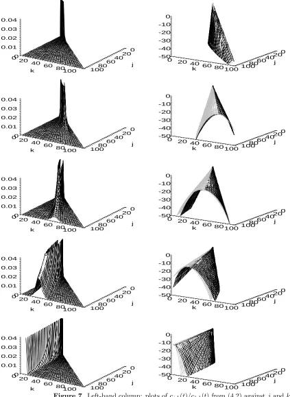
Over this timescale we see the transition from most of the mass being focused around the linek =j to the fully compact state where the distribution has its maximum around the line k = 1. The position of the maximum being given by k=θc(T)j =je

−γt

. The solution at large cluster times at large times is illustrated in Figure 7, where γ/a%= 10−2

, at times t = 4, 30, 70, 140, 400. In the top graphs, the mass can be seen to lie predominantly along the linek =j, which in successive graphs moves tok= 0.74j at t = 30, k = 0.50j at t = 70,k = 0.25j att = 140, the ratios k/j agreeing well with e−t/100

. Att= 400, we find almost all the system’s mass along the linek= 1; consistent with the prediction θ =k/j = e−4

≈ 0.02. Simultaneous with this change in shape of the clusters, we observe a steady increase in size as the distribution evolves from a large and sharply-peaked maximum atj = 1 to much lower concentrations over a broad range of sizes.

At even longer timescales, whent1/γ, the system is dominated by fully compact clusters, that is, clusters of the form Cj,1. For large j we have the similarity solution

cj,1(t)∼4e

−2j/a%t

/a2%t2, (4.20)

and cj,2(t)∼je

−γt

cj,1(t), thus cj,2(t)cj,1(t).

4.7. Compaction and aggregation on similar timescales

0 20

0 ₄₀

0 0.01

20 ₄₀ 60 j 0.02 60 80 80 0.03 100 k 100 0.04 0 20 0 ₄₀ 0 0.01

20 ₄₀ 60 j 0.02 60 80 80 0.03 100 k 100 0.04 0 20 0 ₄₀ 0 0.01

20 ₄₀ 60 j 0.02 60 80 80 0.03 100 k 100 0.04 0 20 0 ₄₀ 0 0.01

20 ₄₀ 60 j 0.02 60 80 80 0.03 100 k 100 0.04 0 20 0 ₄₀ 0 0.01

20 ₄₀ 60 j 0.02 60 80 80 0.03 100 k 100 0.04 0 20 -50 0 40 -40 20 -30 60 40 j -20 60 -10 80 0 80

k 100 100

0 20 -50 0 40 -40 20 -30 60 40 j -20 60 -10 80 0 80

k 100 100

0 20 -50 0 40 -40 20 -30 60 40 j -20 60 -10 80 0 80

k 100100

0 20 -50 0 40 -40 20 -30 60 40 j -20 60 -10 80 0 80

k 100 100

0 20 -50 0 40 -40 20 -30 60 40 j -20 60 -10 80 0 80

k 100 100

Figure 7. Left-hand column: plots ofcj,k(t)/c1,1(t) from (4.2) againstj andk.

Right-hand column: plots of logcj,k(t) in black and in grey, the approximation (4.19).

the large-time asymptotic solution of (4.1)–(4.2) will lead to a solution in which the maximally compact clusters dominate all others (cj,k(t)cj,1(t) for all k ≥2) and the size-distribution has the self-similar form cj,1(t) = 4e

−2j/a%t

/a2_%t2_. For largej, k with k =θj and time taken to be _O(1), we have

cj,k(t) ∼

4%√θejH(θ,t)

q

2πj(1₋θ) (2 +a%t)[(2 +a%t)(e−γt

+_E(t))₋2], (4.21)

H(θ, t) = θlog e−γt

+_E(t)₋ 2 2 +a%t

!

−θlogθ₋(1₋θ) log(1₋θ)

+ (1₋θ) log(1₋e−γt

− E(t)). (4.22)

As with (4.15), the dominant term in the expression forcj,k(t) is ejH(θ,t) and H(θ, t) has

a maximum θc(t) which is independent of j, that is, the transformation from extended

(θ = 1) to compact (θ= 0) clusters occurs at the same time for all cluster sizes. This is given by solving Hθ(θ, t) = 0 and leads to

θc(t) =

(2 +a%t)(e−γt

+_E(t))₋2

a%t . (4.23)

However, there is no simplification of the expression for H(θc(t), t) and so no

straightforward approximation for cj,k(t) is available.

5. Discussion

We have formulated a model of cluster growth in which both the size (mass) and shape (maximum diameter) of clusters are explicitly and independently taken into account. The form of the resulting model is that of a multi-component aggregation problem with an additional restructuring process which we have referred to as ‘compaction’ by which a cluster’s maximum diameter is reduced while its mass is left unchanged.

The model is approximated by simplifying the range of maximum diameters allowed from (6j/πσ)1/3 _{≤ k ≤ j to 1 ≤ k ≤ j where k is the maximum diameter of a cluster} of mass j, density σ and hence volume j/σ. Following certain assumptions on the form of the rate coefficients, we have obtained a model which is solvable explicitly using analytical techniques. The resulting solution can be used to check numerical solvers of multi-component systems.

2 4 6 0 j 2 0.002 8 4 0.004 6 ₈ 0.006 10 10 0.008 k 0.01 2 4 6 0 j 2 0.002 8 4 0.004 6 ₈ 0.006 10 10 0.008 k 0.01 2 4 6 0 j 2 0.002 8 4 0.004 6 ₈ 0.006 10 10 0.008 k 0.01 2 4 6 0 j 2 0.002 8 4 0.004 6 ₈ 0.006 10 10 0.008 k 0.01 2 4 6 _j -50 2 -40 8 4 ₆ -30 8 10 -20 10 -10 k 0 2 4 6 _j -16

2 ₄ 8

-12 6 ₈ -8 10 10 -4 k 2 4 6 _j -16

2 ₄ 8

-12 6 ₈ -8 10 10 k -4 2 4 6 _j -20 2 -16 8 4 ₆ -12

8 ₁₀ 10 -8

k -4

Figure 8.Left-hand column: plots ofcj,k(t)/c1,1(t) from (4.2) againstjandk.

Right-hand column: plots of logcj,k(t). Descending in sequence, the plots illustrate the shape

of the distribution at timest= 0.1, 1.1, 2.1, 3.1 for the parameter valuesγ= 1,a= 1,

We have used Matlab to analyse the difference between systems where the maximally compact cluster has a maximum diameter of kc=O(j1/3) and the explicitly

solvable system where kc = 1. The differences are not large, in the former model the

range of maximum diameters allowed at any cluster mass j is j1/3 _{≤ k ≤ j, which we} have approximated by 1_≤k _≤j. For large masses,j, the relative difference is_O(j−2/3

), which is small. However, by incorporating the range from k= 1 to k =_O(j1/3_{) we are} losing some of the geometric information about the allowable structure of clusters. In calculations of the average maximum diameter and fractal dimension, these differences become noticeable, as can be seen in Figure 5, where fractal dimensions of 3 and above are rapidly realised. We have illustrated how an a posteriori rescaling of the results by (3.24)–(3.25) can eliminate the majority of the discrepancy in the calculation of the average diameter and fractal dimension (see Figure 6 for details).

We have chosen monodisperse initial data and simplified the resulting solution using asymptotics; this enables us to illustrate some of the kinetic features of simultaneous aggregation and compaction. For the combination of aggregation kernel and compaction rates adopted here, the large-cluster size asymptotics are particularly simple: the timescale over which compaction occurs is the same for all cluster sizes. We expect that when more general rate coefficients are employed, large and small clusters may restructure over different timescales. For rapid compaction and slow coagulation, the results are straightforward as clusters are always in their most compact form, and grow in size according to the usual self-similar solution. When aggregation is much faster than compaction the kinetics of the solution are more interesting. There is a faster timescale where self-similar growth is seen along the line k = j, that is, linear aggregates form in a self-similar fashion. Over a slower timescale the whole distribution of cluster sizes restructures to the more compact form, whilst continuing to grow in size following the same self-similar rule. For more general rates of growth and shape restructuring one would expect more complex rules, where small and large clusters changed their shape and fractal dimension over differing timescales.

Acknowledgements

I am very grateful to Sotiris Pratsinis and Martin Heine for making many helpful comments following a careful reading of the manuscript.

References

[1] M Abramowitz & IA Stegun. Handbook of Mathematical Functions. Dover, New York, (1972). [2] MK Akhtar, G Lipscomb & SE Pratsinis. Monte Carlo simulation of coagulation and sintering.

Aerosol Sci Technol,21, 83–93, (1994).

[3] M Alonso. Simultaneous charging and Brownian coagulation of nanometre aerosol particles.J Phys A; Math Gen, 32, 1313–1327, (1999).

[5] CM Bender & SA Orszag. Advanced Mathematical Methods for Scientists and Engineers. McGraw-Hill, Singapore, (1978).

[6] CD Bolton & JAD Wattis. The size-templating matrix effect in vesicle formation I: a microscopic model and analysis.J Phys Chem B,107, 7126–7134, (2003).

[7] CD Bolton & JAD Wattis. The size-templating matrix effect in vesicle formation II: a macroscopic models and analysis.J Phys Chem B,107, 14306–14318, (2003).

[8] FP da Costa, M Grinfeld, JAD Wattis. A hierarchical cluster system based on Horton-Strahler rules for River networks.Studies in Applied Mathematics,109, 163–204, (2002).

[9] PV Coveney & JAD Wattis. A Becker-D¨oring model of self-reproducing vesicles.J. Chem. Soc.: Faraday Transactions,102, 233–246, (1998).

[10] SC Davies, JR King & JAD Wattis. Self-similar behaviour in the coagulation equations. J Eng Math,36, 57–88, (1999).

[11] C Elvingson & S Wall. Kinetic of mixed and ionic micelles. A discussion of the slow process and a general formulation of the slow relaxation time.J Phys Chem,90, 5250–5254, (1986). [12] HK Kammler, R Jossen, PW Morrison Jr, SE Pratsinis, G Beaucage. The effect of external electric

fields during flame synthesis of titania.Powder Technol, 135, 310–20, (2003).

[13] M Kostoglou & AG Konstandopoulos. Evolution of aggregation size and fractal dimension during Brownian coagulation.Aerosol Sci,32, 1399–1420, (2001).

[14] M Kostoglou, AG Konstandopoulos & SK Friedlander. Bivariate population dynamics simulation of fractal aerosol aggregate coagulation and restructuring.to appear in Aerosol Sci,37, –, (2006). [doi:10.1016/j.jaerosci.2005.11.009]

[15] A Schild, A Gutsch, H Muehlenweg, D Kerner & SE Pratsinis. Simulation of nanoparticle production in premixed aerosol flow reactors by interfacing fluid mechanics and particle dynamics.J Nanoparticle Res,1, 305–315, (1999).

[16] M von Smoluchowski. Drei vortr¨age ¨uber diffusion Brownsche molekular bewegung und koagulation von kolloidteichen.Physik Z,17, 557–571 (1916).

[17] S di Stasio, AG Konstandopoulos & M Kostoglou. Cluster-cluster aggregation kinetics and primary particle growth of soot nanoparticles in flame by light scattering and numerical simulations.J Colloid & Interface Sci,247, 33-46, (2002).

[18] S Tsantilis & SE Pratsinis. Evolution of primary and aggregate particle size distributions during coagulation and sintering.AIChE J,46, 407–415, (2000).

[19] S Vemury, C Jansen & SE Pratsinis. Coagulation of symmetric and asymmetric bipolar aerosols.

J Aerosol Sci,28, 599–611, (1997).

[20] S Vemury & SE Pratsinis. Self-preserving size distributions of agglomerates. J Aerosol Sci, 26, 175–185, (1995), [Erratum,26, 701, (1995)].

[21] S Wall & C Elvingson. Equilibrium and kinetic properties of mixed micelles.J Phys Chem, 89, 2695–2705 (1985).

[22] JAD Wattis. Exact solutions for two-component aggregation,preprint, (2006).

[23] DT Wu. General approach to barrier crossing in multi-component nucleation.J Chem Phys, 99, 1990–2000, (1993).

[24] Y Xiong & SE Pratsinis. Formation of agglomerate particles by coagulation and sintering: part I. a two-dimensional solution to the population balance equation. J Aerosol Sci, 24, 283–300, (1993).