Force Tracking Control for Motion
Synchronization in Human-Robot
Collaboration
Yanan Li1 and Shuzhi Sam Ge2∗
1 Institute for Infocomm Research, Agency for Science, Technology and Research, Singapore 138632
2 Department of Electrical and Computer Engineering, and Social Robotics Laboratory, Interactive Digital Media Institute, National University of Singapore, Singapore 117576
Abstract: In this paper, motion synchronization is investigated for human-robot collabo-ration such that the robot is able to “actively” follow its human partner. Force tracking is achieved with the proposed method under the impedance control framework, subject to uncertain human limb dynamics. Adaptive control is developed to deal with point-to-point movement, and learning control and neural networks (NN) control are developed to generate periodic and arbitrary continuous trajectories, respectively. Stability and tracking perfor-mance of the closed-loop system are discussed through rigorous analysis. The validity of the proposed method is verified through simulation and experiment studies.
Index Terms – Motion synchronization; human-robot collaboration; force tracking.
1
Introduction
Robots are envisioned not only to co-exist but also to collaborate and co-work with human beings in the foreseeable future. Most industrial tasks that are either too complex to automate or too difficult to operate manually are impractical and even impossible to be solely taken by either fully automated robots or human workers. The thrusts of human-robot collaboration rely on the observation that human workers and robots share the same workspace and have complementary advantages. The robots’ strength lies in their superior efficiency in carrying out regular tasks at the high speed with the guaranteed performance, while human workers with their cognitive skills excel in understanding the circumstances, reasoning, and problem solving.
In this paper, we consider a human-robot collaboration scenario where the human partner leads the robot along a trajectory through a kinesthetic interface. This topic is usually referred to
∗To whom all correspondences should be addressed.
as manual guidance, walk-through programming, or hands-on control in the literature, and has been studied in extensive works such as [1, 2, 3, 4, 5, 6, 7, 8, 9]. In many cases, the robot is expected to “actively” follow the human partner so that the human partner may reduce his/her effort during the collaboration. A typical example is the transport of a heavy load where the robot is expected to share most of the load while the human partner applies a small interaction force to move the robot.
1.1
Related Works
Force/impedance control is an optional framework for analysis of the human-robot collab-oration scenario discussed above. By employing force control, the robot will move along a trajectory to reduce the interaction force between the human partner and the robot [10]. However, the robustness of force control can become a serious issue, especially when there exists switching between free motion and constrained motion phases [11]. Impedance control is demonstrated by previous studies to be able to provide relatively better robustness since it avoids switching between different phases [12, 13]. By employing impedance control, the robot is controlled to be compliant to the force exerted by the human partner. However, as the interaction force is indirectly regulated by impedance control, a small interaction force and thus motion synchronization cannot be achieved in a straightforward way. In this regard, the robot under impedance control will act as a load to the human partner when he/she changes his/her intended motion [3]. To cope with this issue, much effort has been made to realize force tracking under the framework of impedance control [14, 15, 16, 17]. In [14], two adaptive schemes are proposed to achieve force tracking by adjusting the rest position in the impedance model. In [15], an impedance model with zero stiffness is adopted, and the force error is elim-inated by an adaptive scheme subject to uncertainties in robot dynamics and little knowledge of environment dynamics. Instead of adjusting the rest position in the impedance model, the stiffness parameter is updated to achieve force tracking with a small tracking error in [16]. Another popular method for the aforementioned human-robot collaboration scenario is to es-timate human partner’s motion intention by analyzing position and/or force feedback at the interaction point. In research studies such as [4, 5, 6, 18], human partner’s motion charac-teristics is analyzed to generate a collaborative movement for the robot. In [19], the state of human partner’s motion intention is assumed to be a stochastic process, and the hidden Markov model (HMM) is employed for the intention observation. In [7], under the assumption that the momentum is preserved during an interaction task, human partner’s motion intention is represented by the change of the interaction force, which is estimated by the change of the control effort. In our previous work [9], human partner’s motion intention is estimated subject to a unknown human limb model with uncertainties.
1.2
Contributions
In this paper, we employ impedance control and develop force tracking control to achieve human-robot motion synchronization, subject to uncertain human limb dynamics. The mass-damping-stiffness model developed under the equilibrium point control hypothesis will be used to describe the human limb dynamics [20, 21]. This model suggests that the interaction force is resulted due to the error between the actual trajectory and the equilibrium position of the human limb. Therefore, the equilibrium position is deemed as the desired trajectory/motion intention of the human partner, which is planned in the central nervous system (CNS) of the human partner and unknown to the robot. Since this desired trajectory is generally time-varying and uncertain due to the modeling error and external disturbance, it is different from the constant rest position studied in [14, 15, 16, 17]. Three typical cases will be discussed under the same framework: adaptive control will be developed to deal with the point-to-point movement, and learning control and neural networks (NN) control to generate periodic and arbitrary continuous trajectories, respectively. Stability and tracking performance of the closed-loop system will be shown to be guaranteed, even in the presence of active force feedback.
Based on the above discussions, we highlight the contributions of this paper as follows:
(i) A force tracking framework is proposed for the motion synchronization in human-robot collaboration, such that the robot is able to “actively” follow its human partner.
(ii) Adaptive control is proposed to deal with the point-to-point movement, and learning control and NN control are developed to generate periodic and arbitrary continuous trajectories, respectively.
(iii) Human limb dynamics are taken into consideration in the system performance analysis, and it is proved that force tracking is guaranteed subject to uncertain human limb dynamics and active force feedback.
The rest of the paper is organized as follows. In Section 2, the human-robot collaboration system under study is introduced and the control objective of force tracking is discussed. In Section 3, three cases of motion synchronization are discussed and the system performance for each case is rigorously analyzed. Section 4 is dedicated to discuss the system performance when the inner-loop dynamics are considered. In Section 5.1, the simulation study is used to verify the effectiveness of the proposed method. In Section 5.2, further examination of the proposed method is carried out with the practical implementation. Concluding remarks are given in Section 6.
2
Problem Formulation
2.1
System Description
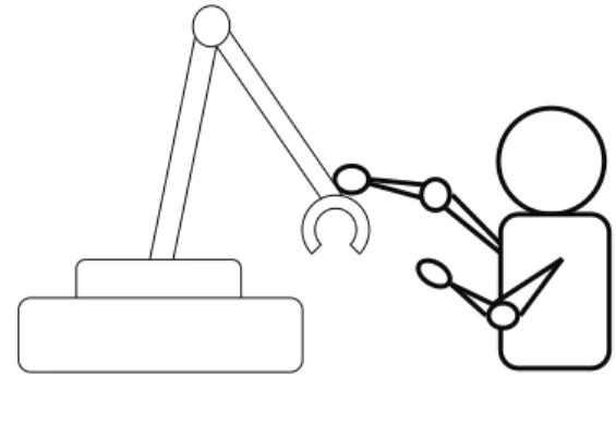
In this paper, we investigate a typical human-robot collaboration system, which includes a robot arm and a human limb, as shown in Fig. 1. The human limb holds the end-effector of the robot arm and aims to move it along a certain trajectory which is unknown to the robot arm. There is a force sensor at the end-effector of the robot arm which measures the interaction force between the human limb and robot arm.
Figure 1: System under study
Consider the robot kinematics given by
X(t) =φ(q) (1) whereX(t)∈Rn and q ∈Rn are positions/oritations in the Cartesian space and joint
coordi-nates in the joint space, respectively. Differentiating (1) with respect to time results in ˙
X(t) =J(q) ˙q (2) whereJ(q)∈Rn×nis the Jacobian matrix and assumed to be nonsingular in a finite workspace.
The robot arm dynamics in the joint space are described as
M(q)¨q+C(q,q˙) ˙q+G(q) =u+JT(q)F(t) (3) where M(q)∈Rn×n is the symmetric bounded positive definite inertia matrix; C(q,q˙) ˙q ∈
Rn denotes the Coriolis and Centrifugal force;G(q)∈Rn is the gravitational force; u∈
Rn is the vector of control input; and F(t) ∈ Rn is the measured interaction force. Note that F(t) is
also the force exerted by the human limb, from the point of view of the robot arm.
The other part of the system under study is the human limb. As discussed in Introduction, the equilibrium point control hypothesis has been proposed to describe human limb dynamics in the literature, which results in a mass-damping-stiffness model [20]. As the damping and
stiffness components dominate the human limb dynamics [21], the following simplified model is employed
F =ChX˙ +Kh(X−Xh) + ∆(X,X˙) (4)
where Ch and Kh are unknown damping and stiffness matrices, Xh is the desired trajectory
generated by the CNS and ∆(X,X˙) is the uncertainty, which may be resulted by incomplete modeling, time-varying property of Ch and Kh, and external disturbance.
2.2
Control Objective
In a predefined task, the desired trajectory of the robot arm is prescribed and available for the control design. In a human-robot collaboration task under study in this paper, the desired trajectory is determined by the human partner and unknown to the robot arm. Impedance control is adopted in such a way that the robot arm is controlled to be compliant to the interaction force between the human limb and robot arm. Equivalently, a desired impedance model of the robot arm is given by
Md( ¨Xd−X¨0) +Cd( ˙Xd−X˙0) +Gd(Xd−X0) =−F (5) where X0 is the rest position, Md, Cd and Gd are desired inertia, damping and stiffness
matrices, respectively, and Xd is the desired trajectory calculated according to (5).
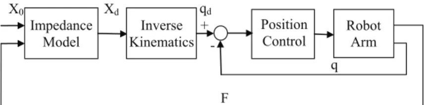
A two-loop control framework is usually used to achieve impedance control which is shown in Fig. 2. In this framework, the outer-loop is dedicated to generate qd =
Rt
0 J−
1(q(τ)) ˙X
d(τ)dτ
according to the measured interaction forceF and the impedance model (5). The inner-loop is to guarantee the trajectory tracking, i.e., limt→∞q(t)→qd(t), which can be achieved by the
following adaptive control [22]
u=Y(¨qr,q˙r,q, q˙ ) ˆΥ +Kr+JT(q)F (6)
where K is a positive definite matrix, ˆΥ is the estimation of Υ and updated as
˙ˆΥ = ΓYT(¨qr,q˙r,q, q˙ )r (7) with Γ>0, and ˙ qr = q˙d+αe with e=qd−q r = ˙e+αe (8) with α >0.
Robot Arm + Position Control F q Impedance Model qd -Inverse Kinematics Xd X0
Figure 2: Impedance Control Diagram
Remark 1 Tracking control has been extensively studied in the literature, and adaptive control in [22] is adopted above for its well-known capability in handling parametric uncertainties. Other control methods (e.g., independent joint control which is the standard approach adopted in industrial robot controllers) can be also used under the framework proposed in this paper, as long as the trajectory tracking in the inner-loop is guaranteed.
Adaptive control (6) only guarantees asymptotic tracking, i.e., limt→∞q(t)→qd(t). However,
in the first part of this paper, we assume that perfect tracking is guaranteed by the inner-loop control, i.e., q=qd. Thus, we have X=Xd and the following impedance model
Md( ¨X−X0¨ ) +Cd( ˙X−X0˙ ) +Gd(X−X0) =−F (9)
Interpreting the impedance model (9), we find that the interaction force F is generated by the error between the actual position of the robot arm X and the rest positionX0. Seen from the perspective of the human partner, he/she will feel like moving an object with inertial/massMd,
damping Cd and stiffnessGdfromX0 toX, as shown in Fig. 3. Obviously, it is expected that
F should be made as small as possible to free the human partner from a large load. One way to achieve this is to choose small impedance parameters, which may, however, cause system instability [9]. Another way is to design X0 to make it get close toX, which is the motivation of the work in this paper. This will lead to motion synchronization, which is referred to as “active” following. Md Cd Gd F X0 X
3
Motion Synchronization
By choosing Md, Cd and Gd to be diagonal matrices, we consider the system dynamics in a
single direction. In particular, we use md, cd, gd, x, x0, f, ch, kh, xh and δ to represent a
component of Md, Cd,Gd, X, X0,F, Ch, Kh, Xh and ∆, respectively.
Considering the impedance model of the robot arm in a single direction
md(¨x−x¨0) +cd( ˙x−x˙0) +gd(x−x0) =−f (10) we have
x=x0−f′ (11)
where the signal f′ satisfies
mdf¨′+cdf˙′+gdf′ =f (12)
It is noted that f′ is a filtered signal of f.
The human limb model in a single direction is given by
f =chx˙ +kh(x−xh) +δ(x,x˙) (13)
Property 1 ∂δ∂x and ∂∂δx˙ are bounded, and|δ(x,x˙)|< k1|x|+k2|x˙|, wherek1 andk2are unknown
positive constants.
Remark 2 Property 1 indicates that the uncertainty of human limb impedance, i.e., damping and stiffness, is bounded.
By substituting (11) into (13), we obtain f kh = x−xh + chx˙ kh + δ(x,x˙) kh =x0−f′−x h+ chx˙ kh +δ(x,x˙) kh (14) Then, we design x0 =f′+ ˆxh−ˆchx˙ +xδ (15)
where ˆxh and ˆch are the estimates of xh and ckh
h, respectively, and
xδ = ˆk1sgn(xf)x+ ˆk2sgn( ˙xf) ˙x (16)
with ˆk1 and ˆk2 as the estimates of k1
kh and
k2
kh, respectively. It will be shown in the analysis
below that xδ is used to compensate for δ(x,x˙)
According to (14) and (15), we have f kh = ˜xh−˜chx˙ + (xδ+ δ(x,x˙) kh ) (17) where ˜xh = ˆxh−xh and ˜ch = ˆch− kch h. Lemma 1 (xδ+δ(kx,x˙) h )f ≤ − ˜ k1sgn(xf)xf−k2˜ sgn( ˙xf) ˙xf, where˜k1 = ˆk1−k1 kh and ˜ k2 = ˆk2−k2 kh.
Proof 1 See Appendix 7.1.
In the following, we discuss three cases where xh is assumed to be constant, periodic and
arbitrary continuous, respectively. Motion synchronization in each case is achieved, i.e., to design x0 in (15) to make limt→∞f = 0.
3.1
Point-to-Point Movement
In the case of point-to-point movement, i.e.,xhis a constant, we develop the following updating
law
˙ˆ
xh =−γf, c˙ˆh =−γxf,˙ k˙ˆ1 =−γsgn(xf)xf, k˙ˆ2 =−γsgn( ˙xf) ˙xf (18) where γ is a positive scalar.
Theorem 1 Considering the closed-loop dynamics described by (17), the rest position (15) with the updating law (18) guarantees the following results:
(i) the interaction force asymptotically converges to 0 as t→ ∞, i.e., lim
t→∞f(t) = 0, and
(ii) all the signals in the closed-loop system are bounded.
Proof 2 See Appendix 7.2.
3.2
Periodic Trajectory
It is noted that xh in the the previous section is assumed to be a constant, which is valid in
the case of point-to-point movement. However, in many practical applications,xh is usually a
time-varying trajectory. Therefore, this section is dedicated to discuss the case of time-varying trajectory. From the performance analysis in the previous section, it is found that the adaptive method is not applicable to the case of time-varying trajectory. In particular, the existence of ˙xh will result in the interaction force. In the following, we develop an iterative learning
Assumption 1 The desired trajectory of the human limb xh is periodic with a known period
T, i.e.,
xh(t) =xh(t−T), xh(t) = 0, t <0 (19)
Considering the rest position (15), we replace the updating law for ˙ˆxh in (18) by the following
learning law
ˆ
xh(t) = ˆxh(t−T)−γf, xˆh(t) = 0, t <0 (20)
Theorem 2 Considering the closed-loop dynamics described by (17), the rest position (15) with the updating laws (18) and (20) guarantees the following results:
(i) the interaction force asymptotically converges to 0 as t→ ∞, i.e., lim
t→∞f(t) = 0, and
(ii) all the signals in the closed-loop system are bounded.
Proof 3 See Appendix 7.3.
Remark 3 In the case discussed in this section, xh is assumed to be periodic and learning
control is thus developed. For learning control, usually the repositioning condition is required [23], i.e., the robot arm is required to move to the initial position at the beginning of each period. To relax this assumption, much effort has been made by adopting alignment condition instead, i.e., the robot arm is only required to start from where it stops [24]. Motivated by adaptive learning control in [25], the method proposed in this paper requires neither the repositioning condition nor the alignment condition, which has been shown in the above proof.
3.3
Arbitrary Continuous Trajectory
In the previous section, it is assumed in Assumption 1 that xh is periodic, which obviously
limits the applications of the proposed method. In this section, we make use of the linearly parameterized function approximators to relax this assumption. The basic idea is to approxi-mate an arbitrary continuous trajectory by a linearly parameterized function, and the adap-tive method is developed to estimate the ideal weights. Radial basis function neural networks (RBFNN) is employed in this paper as the linearly parameterized function approximator. Observing the human limb model (13), xh can be determined by f, x and ˙x. Therefore, we
have the following assumption:
Considering the rest position (15), we replace the updating law for ˆxh in (18) by the following updating law ˆ xh = p X i=1 ˆ wisi(z)−sgn(f)ε ˙ˆ wi = −γsif, for i= 1, . . . , p (21)
The following analysis will show that sgn(f)ε is to compensate for the NN modeling error. Theorem 3 Considering the closed-loop dynamics described by (17), the rest position (15) with the updating laws (18) and (21) guarantees the following results:
(i) the interaction force asymptotically converges to 0 as t→ ∞, i.e., lim
t→∞f(t) = 0, and
(ii) all the signals in the closed-loop system are bounded.
Proof 4 See Appendix 7.4.
4
Inner-Loop Dynamics
In the above analysis, it is assumed that perfect tracking is achieved by the inner-loop position control, i.e., X = Xd. As a matter of fact, the position control mentioned in Section 2 only
guarantees the asymptotic tracking, i.e. limt→∞q(t) = qdand thus limt→∞X(t) =Xd. In this
regard, we need to take the inner-loop dynamics into account and investigate if it affects the result of force tracking. In particular, by denotingE =Xd−X, we evaluate the force tracking
performance under the following condition: limt→∞E(t) = 0 and E ∈L2. Similar discussions about this issue can be found in [26].
Instead of (10), the impedance model is given by
md(¨xd−x¨0) +cd( ˙xd−x˙0) +gd(xd−x0) = −f (22) Accordingly, we have xd = x0 −f′ instead of (11). Then, instead of (17), the closed-loop dynamics including the human limb dynamics (13) become
f kh = ˜xh−˜chx˙+ (xδ+ δ(x,x˙) kh )−e (23)
where e represents a component of E. Note that e cannot be measured because xd is a part
of the control input.
Lemma 2 The results in Theorems 1, 2 and 3 are guaranteed if limt→∞e(t) = 0 and e∈L2. Proof 5 See Appendix 7.5.
5
Simulation and Experiment
5.1
Simulation Study
In this section, we consider a human-robot collaboration system, which includes a human limb and a robot arm. The human limb grasps the end-effector of the robot arm and the interaction force is measured by the sensor mounted at the end-effector. The robot arm is under position control in the joint space and its desired trajectory is obtained by the method developed in this paper. Three cases will be discussed and the desired trajectory of the human limb will be a point-to-point movement, a periodic trajectory and an arbitrary continuous trajectory, respectively. To illustrate the advantage of the proposed method over the “passive” method, damping control (i.e., impedance control with zero stiffness) is used for the comparison purpose. The simulation is conducted with the Robotics Toolbox [27].
The robot arm includes two revolute joints and its parameters are: m1 = m2 = 2.0kg, l1 = l2 = 0.2m, I1 = I2 = 0.027kgm2, l
c1 = lc2 = 0.1m, where mi, li, Ii, lci, i = 1,2, represent the
mass, the length, the moment of inertia about the z-axis that comes out of the page passing through the center of mass, and the distance from the previous joint to the center of mass of linki, respectively. Note that these parameters are only used for the simulation and they will not be used in the control design. The initial positions of the robot arm are q1 = −π3 and q2 = 23π. It is assumed that the human limb exerts the force only in X direction and thus the robot arm in Y direction is interaction-free. Nevertheless, note that in the inner position control loop, the dynamics in two directions are still coupled, i.e., the control performance in one direction still affects that in the other direction. The human limb model is described by f = ˙x+ 50(x−xh)−01+.4xx−2+ ˙0.x1 ˙2x, where the last component
0.4x−0.1 ˙x
1+x2+ ˙x2 stands for the uncertainty.
As mentioned above, this uncertainty is a function of x and ˙xsatisfying Property 1, and it is resulted by incomplete modeling of the human limb and time-varying property of Ch andKh.
By adopting the computed-torque control in Section 2, we setY = [¨qr1,2 cos(q2)¨qr1+cos(q2)¨qr2− sin(q2) ˙qr1 −sin(q2)(2 ˙q1 + ˙q2) ˙qr2,q¨r2; 0,cos(q2)¨qr1 + sin(q2) ˙q1q˙r1,q¨r1 + ¨qr2]. The parameters in (8), (6) and (7) are α= 1, K = diag[5,7.5] and Γ = diag[0.5,0.5,0.5]. And the updating ratio in (18), (20) and (21) is γ = 0.01. The damping parameter in impedance control is 150. In the first case, the desired trajectory of the human limb (motion intention) is xh = 0.25
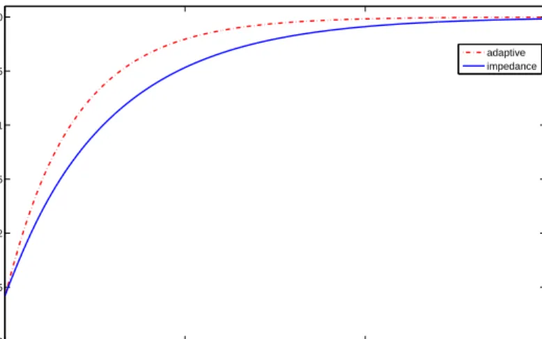
and the updating law (18) is applied. The results in this case are shown in Figs. 4-8. In Fig. 4, it is shown that the positions of the robot arm with both impedance control and the proposed adaptive method track the motion intention. Accordingly, it is found in Fig. 5 that the interaction forces with both methods go to zero. It indicates that human-robot collaboration can be achieved with both methods in the case of point-to-point movement. Nevertheless, it is also noted that the responsive time with the proposed adaptive method is shorter, which illustrates that the robot arm follows human partner more “actively” with the
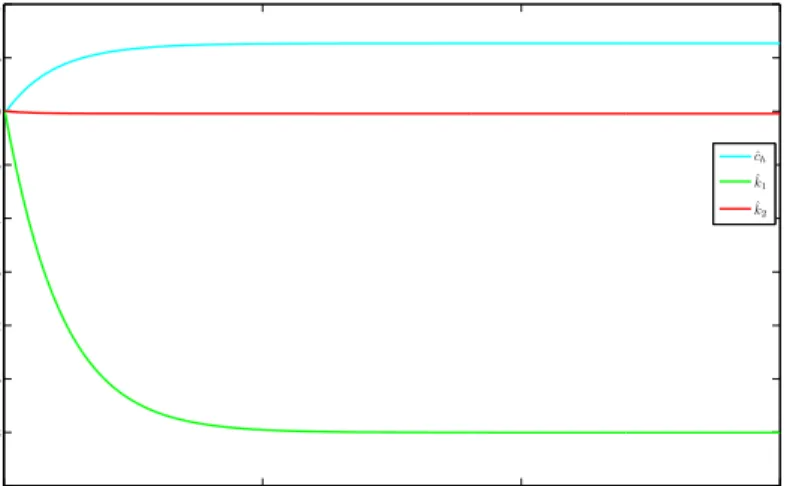
proposed adaptive method. The result of the adaptation parameters is shown in Fig. 6, where the parameters converge to some constants. The control performance of the inner position control loop is also investigated and the results are shown in Figs. 7 and 8. Fig. 7 shows that the tracking error goes to zero and Fig. 8 illustrates the convergence of the adaptation parameters. 0 500 1000 1500 0.19 0.2 0.21 0.22 0.23 0.24 0.25 0.26 time(0.01s) position(m) intention adaptive impedance
Figure 4: Position in the case of point-to-point movement
0 500 1000 1500 −3 −2.5 −2 −1.5 −1 −0.5 0 time(0.01s) interaction force(N) adaptive impedance
Figure 5: Interaction force in the case of point-to-point movement
In the second case, we consider that the desired trajectory of the human limb is time-varying and periodic, which is given by xh = 0.2 + 0.1 sin(π2t). The updating law (20) is adopted
and the results are shown in Figs. 9 and 10. In Fig. 9, it is shown that after several iterations, the position of the robot arm tracks the motion intention. In Fig. 10, it is shown that the interaction force becomes smaller as the iteration number increases. The control performance of the robot arm under impedance control is actually the control performance in the first iteration under the proposed learning method. The better performance (smaller
0 500 1000 1500 −3.5 −3 −2.5 −2 −1.5 −1 −0.5 0 0.5 1x 10 −3 time(0.01s) adaptation parameters ˆ ch ˆ k1 ˆ k2
Figure 6: Adaptation parameters
0 500 1000 1500 −1.5 −1 −0.5 0 0.5 1 1.5 2 2.5 3x 10 −3 time(0.01s) tracking error(rad) e 1 e2
Figure 7: Tracking error of the inner position control loop
0 500 1000 1500 0 2 4 6 8 10 12x 10 −5 time(0.01s) adaptation parameters ϒ1 ϒ2 ϒ3
tracking error and smaller interaction force) after the first iteration indicates the advantage of the proposed learning method over impedance control. The control performance of the inner position control loop is similar to that in Figs. 7 and 8, and is thus omitted. Note that the point-to-point movement in the first case can be considered as a special case of the periodic time-varying trajectory, so the updating law (20) is also applicable in the first case. In this regard, the updating law (20) can be used in a more general class of applications.
0 200 400 600 800 1000 1200 1400 1600 1800 2000 0.1 0.15 0.2 0.25 0.3 time(0.01s) position(m) intention learning
Figure 9: Position in the case of periodic trajectory
0 200 400 600 800 1000 1200 1400 1600 1800 2000 −4 −3 −2 −1 0 1 2 3 4 time(0.01s) interaction force(N)
Figure 10: Interaction force in the case of periodic trajectory
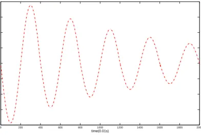
In the last case, we consider an arbitrary continuous trajectory and illustrate that the updating law (21) is applicable in this more general case. The desired trajectory of the human limb is the same as in the second case, which is given by xh = 0.2 + 0.1 sin(π2t). Only one period
is considered so it is non-periodic. The results of trajectory tracking and interaction force are shown in Figs. 11 and 12 respectively, which validate that the proposed NN method guarantees the robot arm to follow the human limb “actively”. Comparatively, impedance
control fails to follow the human limb “actively” because an interaction force of around 5N is needed. Note that the point-to-point movement and periodic trajectory are two special cases of the arbitrary continuous trajectory, so the NN method in the third case is also applicable in the first two cases.
0 50 100 150 200 250 300 350 400 0.1 0.15 0.2 0.25 0.3 time(0.01s) position(m) intention NN impedance
Figure 11: Position in the case of arbitrary continuous trajectory
0 50 100 150 200 250 300 350 400 −6 −4 −2 0 2 4 6 time(0.01s) interaction force(N) NN impedance
Figure 12: Interaction force in the case of arbitrary continuous trajectory
5.2
Experiment
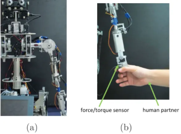
In this section, the proposed method is examined on the robot Nancy which is developed in Social Robotics Laboratory, National University of Singapore [28]. Each joint of Nancy’s arm is implemented using a cable-pulley transmission method which is achieved by a pull-pull configuration. Such a compact configuration reduces the weight and inertia of the robot arm, which is designed considering the better imitation of the human arm. The motor which drives
the joint is precisely controlled by Maxon’s EPOS2 70/10 dual loop controller. It works in the CANopen network and provides multiple operational modes including position, velocity, current modes and others. It also provides the angle information of each joint. An ATI mini-40 force/torque sensor is installed at the left wrist of Nancy. It has a very high signal-to-noise ratio achieved by using silicon strain gages. An industrial PC is used as a global interface. In this experiment, the human partner uses his hand to move the left wrist of Nancy, as shown in Fig. 13. The objective is to make the left wrist of Nancy follow the movement of human limb and the interaction force as small as possible. Different from the simulation, the human partner’s motion intention cannot be measured in the experiment, so the actual trajectory of the robot arm cannot be compared with the motion intention directly. Even if a path (different from the term “trajectory”) can be predefined to follow by the human partner, it cannot represent the human partner’s motion intention. This is because the human partner’s motion intention includes not only the sequence of positions, but also the velocity profile that is very difficult for the human partner to track accurately. In this situation, we can only understand the experiment results through the actual trajectory and external torque. Similarly as in the simulation study, impedance control with zero stiffness is employed for the comparison purpose and impedance parameters in (5) are Md= 0.01, Cd = 0.8 and Gd= 0.
(a)
force/torque sensor human partner
(b)
Figure 13: Nancy and experiment scenario
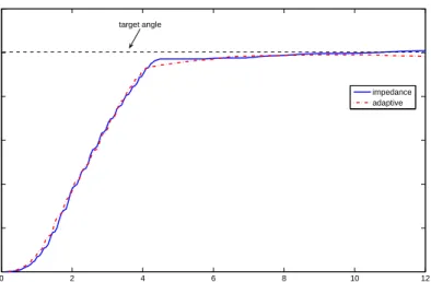
In the first case, Nancy’s wrist is moved to a target angle and the updating law (18) is adopted. The updating ratio is γ = 0.06. The joint angle and external torque are shown in Figs. 14 and 15, respectively. It is found that Nancy’s wrist can be moved to the target angle and the external torque goes to zero. Compared to the result obtained with impedance control, the external torque with the proposed adaptive control is smaller while the performance of the joint angle is similar. This indicates that both the passive method (impedance control) and the proposed adaptive control (18) are applicable in the case of point-to-point movement. However, obviously less effort is needed from the human partner with the proposed method, so the collaboration efficiency can be increased with the proposed method.
In the second case, a periodic trajectory is considered. Particularly, Nancy’s wrist is moved forward and back between two target angles in every 12.6s. The updating law (20) with the
0 2 4 6 8 10 12 0 5 10 15 20 25 30 time(s) joint angle(degree) impedance adaptive target angle
Figure 14: Joint angle in the case of point-to-point movement
0 2 4 6 8 10 12 −0.05 0 0.05 0.1 0.15 0.2 0.25 0.3 time(s) external torque(Nm) impedance adaptive
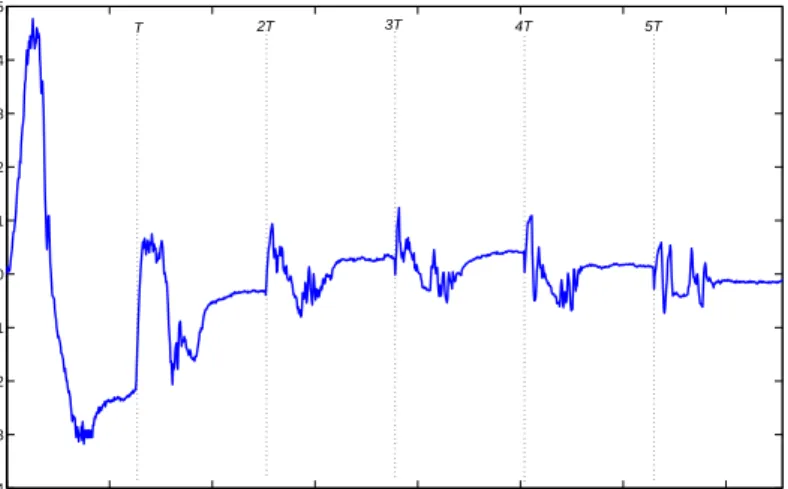
updating ratio γ = 0.36 is employed in this case. The results are shown in Figs. 16 and 17. Similarly as in the simulation study, the control performance of the robot arm under impedance control is the control performance in the first iteration under the proposed learning method. As shown in Fig. 17, Nancy’s wrist in the first iteration is very “stiff” and an external torque of around 0.4Nm is needed. As the iteration number increases, the external torque becomes smaller. At the 6th iteration, an external torque of smaller than 0.1Nm is needed to move Nancy’s wrist to the target angles. These results indicate that Nancy’s wrist starts “actively” following human partner’s motion intention after several iterations. And the validity of the learning method is verified.
0 10 20 30 40 50 60 70 −8 −6 −4 −2 0 2 4 6 8 10 12 time(s) joint angle(degree) target angle 1 target angle 2 T 2T 3T 4T 5T
Figure 16: Joint angle in the case of periodic trajectory
0 10 20 30 40 50 60 70 −0.4 −0.3 −0.2 −0.1 0 0.1 0.2 0.3 0.4 0.5 time(s) external torque(Nm) T 2T 3T 4T 5T
Figure 17: External torque in the case of periodic trajectory
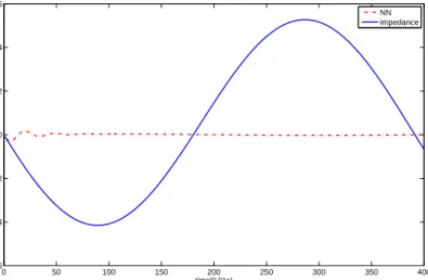
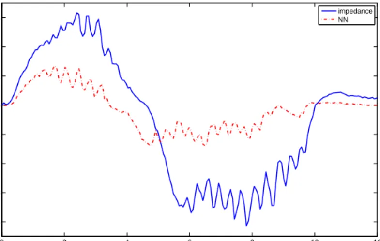
In the third case, Nancy’s wrist is still moved forward and back between two target angles. Because only one period is considered so it is a non-periodic trajectory. As discussed above, this stands for a more general situation. The NN method is employed and the updating law
(21) is adopted with the following parameters: p= 10, ηi = 1, µi = 0, γ = 0.01. The results
in this case are shown in Figs. 18 and 19. It is found that the proposed NN method leads to a faster response and a smaller external torque, compared to impedance control with zero stiffness. Therefore, the proposed NN method is able to make the robot arm “actively” follow its human partner, even in the case of a non-periodic trajectory.
0 2 4 6 8 10 12 −25 −20 −15 −10 −5 0 5 10 15 20 25 30 time(s) joint angle(degree) impedance NN target angle 1 target angle 2
Figure 18: Joint angle in the case of arbitrary continuous trajectory
0 2 4 6 8 10 12 −0.4 −0.3 −0.2 −0.1 0 0.1 0.2 0.3 time(s) external torque(Nm) impedance NN
Figure 19: External torque in the case of arbitrary continuous trajectory
5.3
Discussion
It is essential to understand that the results of relatively smaller external torques in Figs. 15, 17 and 19 are not due to the reason that only the human partner reduces the torques, because otherwise the motion responses of the robot arm would be relatively slower. Figs. 14-19 show results of smaller torques, and at the same time, equalling fast or even faster motion responses, which indicate that the proposed method takes effect.
It is also noted that a small external torque of about 0.1Nm still exists in Fig. 19, which is different from that claimed in Theorem 3 and the simulation results. This may be explained by the following fact. During the experiments, we note that the human partner may change his motion intention according to robot trajectory. This is an interesting issue but was not considered when developing the proposed method. In particular, we assume implicitly that the human motion intention is stationary with respect to the actual robot trajectory, i.e., the adaptation of the robot trajectory has no effect on the human motion intention. However, human motion is also an output of the neuromuscular control system, so the dynamic interac-tion with the robot could well result in concurrent adaptainterac-tions in the human mointerac-tion inteninterac-tion. This makes the problem more tricky and it needs to be further investigated in the future work.
6
Conclusion
In this paper, motion synchronization has been investigated for human-robot collaboration, such that the robot is able to “actively” follow its human partner. Force tracking has been achieved under the impedance control framework, subject to uncertain human limb dynamics. Adaptive control has been proposed to deal with the point-to-point movement, and learning control and NN control have been developed to generate periodic and arbitrary continuous trajectories, respectively. The stability and tracking performance of the whole coupled system have been discussed through the rigorous analysis. The validity of the proposed method has been verified through simulation and experiment studies.
7
Appendix
7.1
Proof of Lemma 1
Considering Property 1 and (16), we obtain
(xδ+ δ(x,x˙) kh )f ≤ xδf+| δ(x,x˙) kh || f| ≤ xδf+ ( k1 kh| x|+ k2 kh| ˙ x|)|f| = xδf+ [ k1 kh sgn(xf)xf + k2 kh sgn( ˙xf) ˙xf] = −˜k1sgn(xf)xf−k˜2sgn( ˙xf) ˙xf (24) It completes the proof.
7.2
Proof of Theorem 1
Denote θ = [xh,kch h, k1 kh, k2 kh] T, ˆθ= [ˆx h,ˆch,ˆk1,ˆk2]T, ˜θ = [˜xh,c˜h,˜k1,k2˜ ]T and φ= [1,x,˙ sgn(xf)x,sgn( ˙xf) ˙x]T (25)Then, according to (18), we have
˙ˆ
θ=−γφf (26)
Consider a Lyapunov function candidate
V1 = 1 2γθ˜
Tθ˜ (27)
Considering θ˙˜=θ˙ˆ, (26), (17) and Lemma 1, the derivative ofV1 with respect to time is ˙ V1 = 1 γθ˜ Tθ˙˜ = 1 γθ˜ T ˙ˆ θ = −θ˜Tφf ≤ −[˜xh−˜chx˙ + (xδ+ δ(x,x˙) kh )]f = −f 2 kh ≤ 0 (28)
AsV1 is positive definite, the above equation shows that V1 ∈L∞. According to the inequality ˙ V1 ≤ −f 2 kh, we have Rt 0 f(τ)2
kh dτ ≤V1(0)−V1(t)≤V1(0), which indicates thatf ∈L2andf ∈L∞.
According to (10) and (13), we have ( ˙x−x˙0)∈L∞and ˙x∈L∞respectively, and thus ˙x0 ∈L∞. Taking derivative of (15) with reference to time, we obtain ˙x0 = ˙f′ + ˙ˆxh −c˙ˆhx˙ −ˆchx¨+ ˙xδ,
and thus ¨x ∈ L∞. Considering Property 1 and ˙δ(x,x˙) = ∂δ ∂xx˙ +
∂δ
∂x˙x¨, we have ˙δ(x,x˙) ∈ L∞. Taking derivative of (13) with reference to time, we have ˙f = chx¨+kh( ˙x−x˙h) + ˙δ(x,x˙).
Thus, ˙f ∈L∞ and f is uniformly continuous. According to Barbalet’s lemma, f ∈L2 and the uniform continuity of f lead to f →0 when t→ ∞. This completes the proof.
7.3
Proof of Theorem 2
Denote ξ = [ch kh, k1 kh, k2 kh] T, ˆξ= [ˆc h,k1,ˆ k2ˆ ]T, ˜ξ = [˜ch,˜k1,˜k2]T and ϕ = [ ˙x,sgn(xf)x,sgn( ˙xf) ˙x]T (29)Then, we have
˙ˆ
ξ =−γϕf (30)
Consider a Lyapunov function candidate
V2 =U +W, U = 1 2γξ˜ T˜ ξ, W = ( 1 2λ Rt 0 x˜ 2 h(τ)τ, 0≤t < T; 1 2λ Rt t−T x˜ 2 h(τ)τ, T ≤t <∞. (31)
where λ is a positive scalar.
The derivative of U with respect to time is ˙ U = 1 γξ˜ Tξ˙˜ = 1 γξ˜ Tξ˙ˆ = −ξ˜Tϕf ≤ −[−˜chx˙ + (xδ+ δ(x,x˙) kh )]f = −(f kh − ˜ xh)f (32)
For 0≤t < T, the derivative ofW with respect to time is ˙ W = 1 2λx˜ 2 h = 1 2λ(ˆxh−xh) 2 = 1 2λ(ˆx 2 h−2ˆxhxh+x2h) ≤ 1 2λ(2ˆx 2 h−2ˆxhxh+x2h) = 1 2λ(2ˆxhx˜h+x 2 h) = 1 2λ(−2λx˜hf +x 2 h) = −x˜hf+ 1 2λx 2 h (33)
Therefore, for 0≤t < T, we have ˙ V2 = ˙U + ˙W ≤ −f 2 kh + 1 2λx 2 h (34)
ForT ≤t <∞, the derivative ofW with respect to time is ˙ W = 1 2λ[˜xh(t) 2 −x˜h(t−T)2] = 1 2λ[˜xh(t) 2 −(˜xh(t) +λf)2] = 1 2λ(−2λx˜hf−λ 2f2) = −x˜hf − λ 2f 2 (35)
Therefore, for T ≤t <∞, we have ˙ V2 = U˙ + ˙W ≤ −( 1 kh +λ 2)f 2 (36)
The following is similar to that in the proof of Theorem 1, and thus omitted.
7.4
Proof of Theorem 3
The proof is similar to that of Theorem 1, so we only highlight the differences. First, we denote ϑ = [w1, . . . , wp, ch kh ,k1 kh , k2 kh ]T ˆ ϑ = [ ˆw1, . . . ,wˆp,ˆch,ˆk1,ˆk2]T ˜ ϑ = [ ˜w1, . . . ,w˜p,c˜h,˜k1,˜k2]T ψ = [s1, . . . , sp,x,˙ sgn(xf)x,sgn( ˙xf) ˙x]T (37) Then, we obtain ˙ˆ ϑ=−γψf (38)
Consider a Lyapunov function candidate
V3 = 1 2γϑ˜
Tϑ˜
The derivative of V3 along the time is ˙ V3 = 1 γϑ˜ T ˙˜ ϑ = 1 γϑ˜ Tϑ˙ˆ = −ϑ˜Tψf ≤ −[˜xh−˜chx˙ + (xδ+ δ(x,x˙) kh ) + (xh−xN N + sgn(f)ε)]f ≤ −[˜xh−˜chx˙ + (xδ+ δ(x,x˙) kh )]f = −f 2 kh ≤ 0 (40)
The following is similar to that in the proof of Theorem 1, and thus omitted.
7.5
Proof of Lemma 2
Sincee∈L2, we haveRt
0 e2(τ)dτ ≤c, wherecis a positive constant. Consider a Lyapunov-like function V =Vj+ c 4cj − 1 4cj Z t 0 e2(τ)dτ, for j = 1,2,3 (41) where c1 =c3 = k1 h and c2 = 1 kh + λ
2. Then, the derivative of V with respect to time is ˙ V = V˙j − 1 4cj e2 ≤ −cjf2+ef − 1 4cj e2 = −(√cjf− 1 2√cj e)2 ≤0 (42)
Similarly as in the proofs of Theorems 1, 2 and 3, we have limt→∞(√cjf(t)− 2√1c
je(t)) = 0.
Because limt→∞e(t) = 0, we finally obtain limt→∞f(t) = 0, and all the other signals are bounded.
References
[1] O. M. Al-Jarrah and Y. F. Zheng, “Arm-manipulator coordination for load sharing using com-pliant control,” Proceedings of the 1996 IEEE International Conference on Robotics and Au-tomation, pp. 1000–1005, April 1996.
[2] O. M. Al-Jarrah and Y. F. Zheng, “Arm-manipulator coordination for load sharing using variable compliant control,” Proceedings of the 1997 IEEE International Conference on Robotics and Automation, pp. 895–900, April 1997.
[3] K. Iqbal and Y. F. Zheng, “Arm-manipulator coordination for load sharing using predictive control,”Proceedings of IEEE International Conference on Robotics and Automation, pp. 2539– 2544, 1999.
[4] Y. Maeda, H. Takayuki, and A. Tamio, “Human-robot cooperative manipulation with motion es-timation,” inProceedings of the 2001 IEEE/RSJ International Conference on Intelligent Robots and Systems, (Maui, Hawaii, USA), pp. 2240–2245, 2001.
[5] M. M. Rahman, R. Ikeura, and K. Mizutani, “Investigation of the impedance characteristic of human arm for development of robots to cooperate with humans,”JSME International Journal Series C, vol. 45, no. 2, pp. 510–518, 2002.
[6] B. Corteville, E. Aertbelien, H. Bruyninckx, J. D. Schutter, and H. V. Brussel, “Human-inspired robot assistant for fast point-to-point movements,”Proceedings of the 2007 IEEE International Conference on Robotics and Automation, pp. 3639–3644, 2007.
[7] M. S. Erden and T. Tomiyama, “Human-intent detection and physically interactive control of a robot without force sensors,”IEEE Transactions on Robotics, vol. 26, no. 2, pp. 370–382, 2010. [8] L. Bascetta, G. Ferretti, G. Magnani, and P. Rocco, “Walk-through programming for robotic
manipulators based on admittance control,” Robotica, vol. 31, pp. 1143–1153, 2013.
[9] Y. Li and S. S. Ge, “Human-robot collaboration based on motion intention estimation,” IEEE/ASME Transactions on Mechatronics, vol. 19, no. 3, pp. 1007–1014, 2014.
[10] J. H. Chung, “Control of an operator-assisted mobile robotic system,”Robotica, vol. 20, pp. 439– 446, 2002.
[11] R. Z. Stanisic and A. V. Fernandez, “Simultaneous velocity, impact and force control,”Robotica, vol. 27, pp. 1039–1048, 2009.
[12] N. Hogan, “Impedance control: an approach to manipulation-Part I: Theory; Part II: Imple-mentation; Part III: Applications,” Journal of Dynamic Systems, Measurement, and Control, vol. 107, no. 1, pp. 1–24, 1985.
[13] Y. Li and S. S. Ge, “Impedance learning for robots interacting with unknown environments,” IEEE Transactions on Control Systems Technology, vol. 22, no. 4, pp. 1422–1432, 2014.
[14] H. Seraji and R. Colbaugh, “Force tracking in impedanc control,” International Journal of Robotics Research, vol. 16, no. 1, pp. 97–117, 1997.
[15] S. Jung, T. C. Hsia, and R. G. Bonitz, “Force tracking impedance control of robot manipulators under unknown environment,”IEEE Transactions on Control Systems Technology, vol. 12, no. 3, pp. 474–483, 2004.
[16] K. Lee and M. Buss, “Force tracking impedance control with variable target stiffness,” Proceed-ings of the 17th IFAC World Congress, vol. 17, pp. 6751–6756, 2008.
[17] R. Z. Stanisic and A. V. Fernandez, “Adjusting the parameters of the mechanical impedance for velocity, impact and force control,” Robotica, vol. 30, pp. 583–597, 2012.
[18] E. Burdet and T. E. Milner, “Quantization of human motions and learning of accurate move-ments,” Biological Cybernetics, no. 78, pp. 307–318, 1998.
[19] Z. Wang, A. Peer, and M. Buss, “An HMM approach to realistic haptic human-robot interac-tion,” Proceedings of the Third Joint Eurohaptics Conference and Symposium on Haptic Inter-faces for Virtual Environment and Teleoperator Systems, pp. 374–379, 2009.
[20] N. Hogan, “The mechanics of multi-joint posture and movement control,”Biological Cybernetics, vol. 52, no. 5, pp. 315–331, 1985.
[21] T. Tsumugiwa, R. Yokogawa, and K. Hara, “Variable impedance control based on estimation of human arm stiffness for human-robot cooperative calligraphic task,”Proceedings of the 2002 IEEE International Conference on Robotics and Automation, pp. 644–650, 2002.
[22] J. J. E. Slotine and W. Li, “On the adaptive control of robotic manipulators,”The International Journal of Robotics Research, vol. 6, no. 3, 1987.
[23] S. Arimoto, “Learning control theory for robotic motion,” International Journal of Adaptive Control and Signal Processing, vol. 4, no. 6, pp. 543–564, 1990.
[24] M. Sun, S. S. Ge, and I. M. Y. Mareels, “Adaptive repetitive learning control of robotic ma-nipulators without the requirement for initial repositioning,” IEEE Transactions on Robotics, vol. 22, no. 3, pp. 563–568, 2006.
[25] R. Yan, K. P. Tee, and H. Li, “Adaptive learning tracking control of robotic manipulators with uncertainties,” Journal of Control Theory and Applications, vol. 8, no. 2, pp. 160–165, 2010. [26] J. Roy and L. L. Whitcomb, “Adaptive force control of position/velocity controlled robots:
theory and experiment,”IEEE Transactions on Robotics and Automation, vol. 18, no. 2, pp. 121– 137, 2002.
[27] P. I. Corke, “A robotics toolbox for MATLAB,” IEEE Robotics and Automation Magazine, vol. 3, pp. 24–32, Mar. 1996.
[28] S. S. Ge, J. J. Cabibihan, Z. Zhang, Y. Li, C. Meng, H. He, M. R. Safizadeh, Y. B. Li, and J. Yang, “Design and development of nancy, a social robot,” inProceedings of the International Conference on Ubiquitous Robots and Ambient Intelligence, (Incheon, Korea), pp. 568–573, 23-26, November 2011.