Design and Development of an Integrated Mobile Robot System for Use in Simple Formations

University of Denver University of Denver

Digital Commons @ DU

Digital Commons @ DU

Electronic Theses and Dissertations Graduate Studies

6-1-2013

Design and Development of an Integrated Mobile Robot System

Design and Development of an Integrated Mobile Robot System

for Use in Simple Formations

for Use in Simple Formations

University of Denver

Follow this and additional works at: https://digitalcommons.du.edu/etd

Part of the Electrical and Computer Engineering Commons

Recommended Citation Recommended Citation

Brune, Christopher D., "Design and Development of an Integrated Mobile Robot System for Use in Simple Formations" (2013). Electronic Theses and Dissertations. 94.

https://digitalcommons.du.edu/etd/94

DESIGN AND DEVELOPMENT OF AN INTEGRATED MOBILE ROBOT SYSTEM FOR USE IN SIMPLE FORMATIONS

A Thesis Presented to

the Faculty of Engineering and Computer Science University of Denver

In Partial Fulfillment

of the Requirements for the Degree Master of Science

by

Christopher D. Brune June 2013

Author: Christopher D. Brune

DESIGN AND DEVELOPMENT OF AN INTEGRATED MOBILE ROBOT SYSTEM FOR USE IN SIMPLE FORMATIONS

Advisor: Matthew J. Rutherford, Ph.D. Degree Date: June 2013

Abstract

In recent years, formation control of autonomous unmanned vehicles has become an active area of research with its many broad applications in areas such as transportation and surveillance. The work presented in this thesis involves the design and implementation of small unmanned ground vehicles to be used in leader-follower formations. This mechatron-ics project involves breadth in areas of mechanical, electrical, and computer engineering design. A vehicle with a unicycle-type drive mechanism is designed in 3D CAD software and manufactured using 3D printing capabilities. The vehicle is then modeled using the unicycle kinematic equations of motion and simulated in MATLAB/Simulink. Simple mo-tion tasks are then performed onboard the vehicle utilizing the vehicle model via software, and leader-follower formations are implemented with multiple vehicles.

Acknowledgements

I would like to offer my sincere appreciation to all of those at the University of Denver who provided me with the opportunity to complete this work. First of all, I would like to thank my advisors Dr. Matthew Rutherford and Dr. Kimon Valavanis for their careful guidance throughout my degree and for continuing to challenge me throughout my work. Additionally, I would like to thank Dr. Michail Kontitsis and my oral defense committee chair Dr. Robert Stencel for their support in this project. I am also very grateful to all of the people at DU2SRI who have worked with me during the past two years: Gonc¸alo Martins, Allistair Moses, Konstantinos Kanistras, Jonathan Girwar-Nath, Daniele Sartori, Jessica Alvarenga-Veyna, Tanarat Dityam, Florence Mbithi, Nikos Vitzilaios, and Alessan-dro Benini. I have learned a lot from each of them on how to perform quality research. Finally, I would like to thank my friends and family, especially my parents, Robert and Catherine, for their endless love, support, and encouragement throughout this process.

Table of Contents

2.2 The Virtual Structure Method . . . 9

2.3 The Leader-Follower Method . . . 11

3 System Design 17 3.1 Existing Systems . . . 17

3.2 UGV Design Considerations . . . 18

3.2.1 XMOS Microcontroller . . . 20

3.2.2 Servo Motors . . . 20

3.3 First Generation Vehicle Design . . . 22

3.4 Second Generation Vehicle Design . . . 27

3.4.1 Chassis Design . . . 27

3.4.2 Bumper Design . . . 30

3.4.3 Power Budget . . . 32

3.5 Cost Analysis . . . 33

4 Vehicle Kinematics and Control 36 4.1 Kinematic Model . . . 36

4.1.1 Discrete Time Kinematic Model and Control . . . 39

4.2 Trajectory Tracking Control . . . 40

5 Simulation, Experimentation, and Results 49

5.1 Simulation . . . 49

5.1.1 Simulation Results . . . 52

5.2 Implementation . . . 54

5.2.1 Motion Implementation Results . . . 57

5.3 Leader-Follower Formation . . . 59

5.3.1 Leader-Follower Formation Results . . . 60

6 Conclusions and Recommendations 65 6.1 Conclusion . . . 65

List of Tables

3.1 Existing Mobile Robot Systems . . . 18

3.2 Initial Vehicle Components . . . 18

3.3 Additional Nonessential Vehicle Components . . . 19

3.4 Vehicle Power Budget . . . 33

List of Figures

1.1 Commercially Available Hilare-type Mobile Robots . . . 2

1.2 Car-Like Mobile Robots . . . 3

3.1 XMOS XK-1A Development Board and XTAG . . . 21

3.2 Hobby King HK15138 Standard Analog Servo Motor . . . 22

3.3 Vehicle Drawing of Miniature UGV, rev. 1 . . . 23

3.4 Initial Prototype of First Generation Miniature UGV . . . 23

3.5 Miniature UGV SolidWorks Design, Version 1 . . . 24

3.6 3D Printed Chassis . . . 24

3.7 3D Printed Chassis and Bumper . . . 25

3.8 Fully Assembled First Generation Vehicle . . . 26

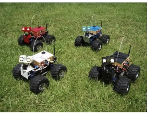
3.9 Initial Fleet of 3D Printed Miniature UGV’s . . . 26

3.10 Assembled Second Generation Vehicle . . . 27

3.11 Second Generation Vehicle with Laser Range Finder . . . 28

3.12 Second Generation Vehicle with Sonar, Compass, and WiFly Antenna . . . 28

3.13 Chassis Re-Design with Standoff Holes . . . 29

3.14 Chassis Top Plate . . . 30

3.15 Chassis Re-Design with Adjusted Servo Mount . . . 30

3.16 Original Bumper Design . . . 31

3.17 Second Generation Bumper Design . . . 31

3.18 Second Generation Bumper Design (angled view) . . . 32

4.1 Schematic of Unicycle-type Mobile Robot [1] . . . 37

4.2 Schematic of Leader-Follower Formation [1] . . . 46

5.1 Unicycle Vehicle MATLAB Model Equations . . . 50

5.2 MATLAB Vehicle Subsystem . . . 51

5.3 Vehicle Trajectory with Constant System Inputs . . . 51

5.4 MATLAB PID Controller for Motion Control . . . 52

5.5 System Response in x-direction . . . 52

5.6 System Response in y-direction . . . 53

5.7 System Response ofθ . . . 53

5.8 Observed Error Over a Circular Trajectory . . . 57

5.10 Leader-Follower Formation with Two Vehicles . . . 61

5.11 Leader-Follower Formation with Three Vehicles . . . 62

5.12 Leader-Follower Formation with Three Vehicles . . . 62

5.13 Alternative Leader-Follower Formation Configuration . . . 63

Chapter 1

Introduction

The topic of this thesis is the study and design of mobile robots and their implementation in simple motion control and formations. There are numerous applications that can utilize formation and cooperative control in robotics. However, there still exist many technolog-ical and scientific challenges before a wide application of multi-vehicle systems becomes feasible. This chapter discusses the motivation and background behind current research in mobile robotics.

1.1

Motivation

In recent years, the study of formation and cooperative control in robotics and unmanned systems has increased in popularity due to its many broad applications [2]. Formation control of autonomous unmanned vehicles has many potential applications. In particu-lar, formation control methods can be used for civilian applications including monitoring, searching, and rescue missions in hazardous environments [3]. It can also be used for mili-tary applications, including reconnaissance and area coverage [4]. Additionally, formations of autonomous vehicles can be used in automated highway systems [5] or other platooning

(a) Parallax Shield-Bot (b) ProtoSnap MiniBot (c) iRobot Roomba Figure 1.1: Commercially Available Hilare-type Mobile Robots

applications such as transportation or mining [6]. Finally, the study of formation control in research has also helped in the understanding of biological systems, such as the swarm-ing of insects or the flockswarm-ing of birds where self-organizswarm-ing and adaptive behaviors can be observed [7] [8].

1.2

Background

1.2.1

Mobile Robots

There exist two common types of mobile robots with well-designed kinematics. These are the unicycle-type and car-like mobile robots. The unicycle-type vehicle, also known as the Hilare-type mobile robot, has two independently driven wheels. These wheels act as the main drive mechanism and are commonly balanced by a passive castor wheel in front or back. In general, this type of vehicle has good maneuvering capability due to its zero minimum turn radius. It is also relatively easy to control. The drawback to this type of vehicle is that it has difficulty driving along a straight trajectory. The unicycle-type vehicle is also easier to design and manufacture due to its simple drive mechanism. Figure 1.1 shows some common unicycle-type mobile robots.

The unicycle-type mobile robot can have different shapes and sizes as can be seen in Figure 1.1. However, the mathematical modeling of such vehicles is typically similar in structure due to the simple drive mechanism that they share. In general, the mathematical models can be adjusted for any unicycle-type mobile robot by using the physical parameters that correspond to that particular vehicle, as long as the modeling assumptions are still valid. The unicycle mobile robot is commonly used in motion control and formation control research.

The other common type of mobile robot is the car-like robot. Like the name suggests, the car-like robot has a drive mechanism that is similar to that of a car. Car-like mobile robots are driven by a single motor that powers a differential. The differential then dis-tributes torque to the rear wheels to move the vehicle. The front wheels contain a steering mechanism that is driven by a motor that generates steering angles to steer the vehicle. A group of small car-like mobile robots can be seen in Figure 1.2. The car-like mobile robot is also commonly found in motion control and formation control research.

1.2.2

Applications

Mobile robot systems have many applications in a number of industries and military en-vironments, and they continue to be a major area of current research in robotics and con-trol. The focus of this thesis is on research involving small unmanned ground vehicles, or UGV’s. Among the numerous applications in mobile robots, there is environment moni-toring and inspection, security and surveillance, and even automated home assisting. Ex-amples include inspecting buildings and trouble sites remotely to reduce emergency visits, map the environment, and avoid obstacles.

In order for unmanned ground vehicles to perform the applications mentioned above, they must be able to perform certain tasks. The vehicle should be able to sense the envi-ronment and obstacles, perform motion planning, and control the drive mechanism so that the physical vehicle is actually able to carry out the planned motion in reality. This the-sis focuses on the physical design of small unmanned ground vehicles, motion control of unicycle-type mobile robots, and the application of vehicles in formation.

1.3

Problem Statement

In this project, we are particularly interested in the problem of existing mobile robot sys-tems being high in cost and relatively complex. Many small mobile robot syssys-tems that currently exist are not ideal for swarm vehicle research due to their overall cost and lack of accommodation with additional sensors for different applications. As a result, there was a desire to create a small unmanned ground vehicle (UGV) to be used for multi-vehicle sys-tems research that was more cost effective than other existing syssys-tems and relatively simple in design. There are a number of mobile robot systems that currently exist, however, most tend to be very expensive and limited by their complexity.

1.4

Contributions

This research focuses on the design and development of a small unmanned ground vehicle (UGV). A small UGV of unicycle-type is designed, and several vehicles are manufactured with focus on small size and low cost. Motion control of the mobile robots is then stud-ied using the vehicle’s kinematic model. This model is then applstud-ied in software onboard the vehicle to operate it using system model inputs. This work is then extended to the implementation of the vehicle in leader-follower formations using sensor-based feedback. The follower vehicles in formation contain a decentralized controller which maintains a particular heading and distance from the vehicle immediately in front of it, also known as the leader. The resulting formation is scalable and useful for further work to be done on formation and cooperative control at the University of Denver’s Unmanned Research Institute.

1.5

Organization of Thesis

This thesis is organized as follows. Chapter 2 provides a literature review where back-ground information on formation and cooperative control is investigated and compared with other existing methods in research. The literature review provides background information on research methods related to formation and cooperative control including behavior-based methods, virtual structure methods, and leader-follower methods. Chapter 3 describes two generations of unmanned ground vehicle that were designed and developed throughout the course of this work. Chapter 4 discusses the theory behind motion control of a unicycle-type mobile robot including kinematic modeling, trajectory tracking, and leader-follower formation control. Chapter 5 describes the simulation, implementation, and results of the designed miniature unmanned ground vehicle in various experiments performed throughout

the course of this project. Finally, Chapter 6 provides conclusions and recommendations for future work.

Chapter 2

Literature Review

Substantial research and development work has been performed in the areas of cooperative and formation control for mobile robots and other unmanned systems. Many technologi-cal challenges involving the development of formation and cooperative control strategies currently exist. These challenges can deal with certain constraints in communication, lo-calization of robot positions, environment mapping such as simultaneous lolo-calization and mapping (SLAM), sensing, learning, and mimicking biological system behaviors such as flocking and schooling.

2.1

The Behavior-Based Method

In literature, there are three different approaches towards formation and cooperative control behavior. The first of these is the behavior-based approach, where several desired behav-iors, such as formation retaining and collision avoidance are prescribed to each vehicle. The vehicle’s final action is then derived by weighing the relative importance of each behavior. A major advantage to this method is that all vehicles in the formation can be controlled in a decentralized fashion. However, the mathematical analysis of this approach tends to be

difficult, and consequently it is not easy to guarantee the convergence of a formation to the desired configuration.

Arkin [4] at the Georgia Institute of Technology presents a behavior-based approach that utilizes reactive behaviors to implement formations in multi-robot teams. The for-mation behaviors used are integrated with navigational behaviors to allow the robot team to reach navigational goals, perform collision avoidance, and simultaneously remain in formation. The behaviors are implemented in simulation as motor schemas within the Autonomous Robot Architecture (AuRA) and as steering and speed behaviors within the Unmanned Ground Vehicle (UGV) Demo II architecture.

Xiaomin et al. introduce a behavior-based high dynamic autonomous formation and control method for use with multi-missile systems [9], which integrates the behavior-based approach with a leader-follower scheme to ensure stability in the formation. The individual behaviors prescribed to each missile include flying toward a destination, holding a forma-tion, obstacle avoidance, and collision avoidance. The appropriate behavior is chosen by a behavior inhibition selection mechanism. The behavior of flying to a destination or leader is achieved by using an optimal route-planning algorithm, which is based on tree topologic data and dynamic programming theory. The behaviors of holding formation and obsta-cle/collision avoidance of followers are achieved by using a global formation-hold control algorithm and obstacle/collision avoidance control algorithm, respectively. This method is implemented in a digital simulation.

In [10], an entrapment/escorting mission is implemented using a kinematic control method based on a new type of behavior-based control known as null space-based be-havioral (NSB) control. This method differs from other existing behavior-based formation control methods in the way that the outputs of the single elementary behaviors are merged to compose the final behavior. The control strategy is validated both in simulation as well as in several experimental cases, where a team of six mobile robots entraps a moving

tar-get represented by a tennis ball that is randomly pushed by hand. In addition, the control approach is made robust so that in the case of one or more vehicle failures, the system can autonomously reconfigure itself to still complete the mission.

Mead et al. in [11] present a behavior-based approach that treats the formation of robots as a type of cellular automation, where each robotic unit is treated as a cell. The robot’s behavior is governed by a set of rules for changing its state with respect to its neighbors. By selecting one of the robots as an initiator, human intervention would change its state, which would propagate to its neighbors, instigating a chain reaction in behaviors from all other robots.

2.2

The Virtual Structure Method

The second approach to formation and cooperative control behavior is the virtual structure approach. In this method, the formation is considered as a virtual rigid structure such as a circle or a square. An advantage to this method is that all vehicles are mutually coupled to each other, however it is often more difficult to determine stability of the formation than other methods. Also, it is necessary for the position and control variables of each individual vehicle or the full state of the virtual structure to be communicated to each individual vehicle in the formation.

A general control strategy for the virtual structure approach is first developed in [12] where control methods force a group of robots to behave as particles that are embedded in a rigid structure. The virtual structure is first aligned with the current position of the indi-vidual robots. The virtual structure is then moved with a certain angle and distance while the individual robots determine desired trajectories that are based on the virtual structure end points. The method is tested using both simulation and experimentation with a group of three robots.

In [13], a virtual structure control method is used for a group of unicycle-type mobile robots using the dynamics of the vehicle model. A combination of path-tracking and the virtual structure approach is used with a small amount of communication between vehicles. An output feedback controller is designed for each individual robot so that a path derivative is left as a free input in order to synchronize the vehicles’ motion. The proposed controller is demonstrated in simulation.

Similarly, a nonlinear formation control architecture is presented in [14], which uses a combination of both virtual structure and path following approaches. A formation con-troller is designed for the kinematic model of two-degree-of-freedom unicycle-type mobile robots and takes into account the physical dimensions and dynamics of the robots. The desired motion for each mobile robot is defined from the motion of the virtual structure’s center while the path following problem for each mobile robot is solved individually by introducing a virtual target that propagates along the path. Coordination of the formation is achieved by synchronizing the parametrization states that capture the positions of the virtual targets with the parametrization states of the virtual structure center.

Another approach to the virtual structure method can be seen in [15] and [16] where a unified, distributed formation control architecture is proposed, which accommodates an arbitrary number of group leaders and allows for arbitrary information flow among vehicles. This method reduces overall complexity to the control law design and analysis due to an extended consensus algorithm that is applied on the group level to estimate the time-varying formation trajectory information. This is done in a distributed manner. Using the estimated formation trajectory information, a consensus-based distributed formation control strategy is then applied for vehicle level control. This proposed formation control architecture is implemented on a multi-robot platform.

In [17], a virtual structure control strategy with mutually coupling between robots is proposed. This controller is designed for nonholonomic unicycle mobile robots and is

based on the vehicle’s kinematic model. Mutual coupling terms are introduced between robots to ensure robustness of the formation in the presence of disturbances. The controller design is validated using experiments with a group of two mobile robots controlled over a wireless communication network.

Additionally in [18], the virtual structure approach is again studied. In this work, the formation control of a group of nonholonomic mobile robots is achieved using implicit and parametric descriptions of the desired formation shape. The presented strategy utilizes implicit polynomial representations to generate potential fields for achieving a desired mation shape. The strategy also utilizes elliptical Fourier descriptors to maintain the for-mation once it has been achieved. Coordination of the vehicles is modeled by linear springs between each vehicle and its two nearest neighbors. This method is scalable to different formation sizes and is validated using simulations with robot groups of different sizes.

2.3

The Leader-Follower Method

The third approach to cooperative and formation control is the leader-follower approach. In this method, some robots are designated as leaders that follow predefined trajectories, while the remaining robots are designated as followers that follow according to a relative position or posture of the leader robot. The main advantage to this approach is that it is relatively easy to understand and implement. Also, it is often less difficult to determine stability with the leader-follower approach than with other methods such as the virtual structure approach [17]. However, this method holds a disadvantage in that there is typically no explicit feedback from the followers to the leader. For example, if a follower is disturbed, the formation cannot be maintained due to the lack of explicit follower feedback. Another disadvantage to this method is that the position of the leader must be communicated to the followers through communication or sensor feedback so that follower robots can use this

information as a control input. This makes the leader-follower more ideal for a centralized control strategy, which is less ideal for a large number of robots.

The focus of this thesis relates to the leader-follower approach with respect to small unmanned ground vehicles. In literature, most designs of formation controllers are based on the kinematic model of nonholonomic unicycle mobile robots. In [5], Desai et al. present a leader-follower formation control method based on local sensor-based information. One robot follows another by controlling relative distance and orientation between itself and the leader. This method is applicable when each follower has only one leader, which allows for the robots to follow in single file. Feedback linearization is used to provide stability to the system, and the method is demonstrated in simulation using six robots.

The idea of using feedback linearization has become common in research with mobile robots with nonholonomic constraints due to their nonlinearity. Many feedback lineariza-tion methods performed have been based on ideas provided in [19], [20], and [21]. This ap-proach is very common in the research of formation control, particularly in leader-follower applications.

Similarly, in [22] and [6], Klanˇcar et al. present a leader-follower method which deals with platoons of wheeled mobile robots with nonholonomic constraints. The control strat-egy presented addresses platooning of a group of wheeled mobile robots that rely on relative sensor information to precisely follow the path of a vehicle in front of it. The vehicles only have local distance and heading information, and there is no explicit communication be-tween vehicles or global information such as GPS. The reference position and orientation of the follower is determined by the estimated path of the leading vehicle. The platoon-ing control strategy presented in this work is validated experimentally usplatoon-ing a group of small-sized mobile robots.

In [23], a second-order kinematic model for a leader-follower type of mobile robot formation is presented. The proposed model is derived in terms of relative motion states

between robots and the follower robot’s local motion. Feedback linearization is then used to achieve the desired formation as well as maintain it. In the proposed control law, accel-eration commands are generated and then converted into velocity inputs for the follower vehicle by multiplying by the control period. Reference velocities for the follower vehicle can then be found by the current velocity to any velocity variations. In addition, an adap-tive controller is developed to add robustness to the system. The adapadap-tive component of the design deals with parametric uncertainty while the robust control component compensates for any uncertainty with the acceleration of the leader robot. The proposed controller is demonstrated in simulation and experimentation.

Another approach to the leader-follower method is introduced in [24] where it is as-sumed that the desired angle between the follower and leader is measured in the follower frame instead of the leader. This method allows for smoother trajectories for the follower as well as lower control effort. Suitable leader conditions for velocity and trajectory are found so that the follower may maintain the formation and satisfy its own velocity constraints. The follower position is not rigidly fixed with respect to the leader.

In [25], a decentralized leader-follower formation controller is proposed for a group of two nonholonomic mobile robots. Using a fixed delay time, the follower tracks the leader’s trajectory with a convenient separation. Only the leader’s position measurement is available for the follower. Simulations are presented to demonstrate the proposed approach.

In [26], the leader-follower problem is formalized in a geometric framework where the properties of the formation are shown to affect the set of admissible curvatures of the leader’s trajectory and the aperture of the cone containing the admissible positions of the follower. The proposed formation is controlled by maintaining a distance and an angle, however, an additional angle is introduced which is referred to the follower and not the leader. Simulation is used to validate the proposed control. Similarly, in [27], a leader-follower scheme is proposed that shows how the geometric properties of the formation

affect the admissible curvatures of the leader’s trajectory as well as the velocity bounds of the followers. The desired angle between the leader and follower is measured in the fol-lower frame and not in the leader frame. The proposed control strategy guarantees smoother trajectories as well as lower control effort and is demonstrated in simulation.

The leader-follower approach is related to the concept of string stability, which can be implemented as a vision-based leader-follower approach such as that presented in [28], [29], and [30] where the follower tracks the leader by means of a camera. The leader-follower approach can also be looked at as in a chained form such as that presented in [31] and [32] which is commonly used in automated highway systems.

It is also popular in literature to perform leader-follower formation control using a vir-tual vehicle approach. A combination of virvir-tual vehicle and trajectory tracking is used to derive formation architecture in [33]. A virtual vehicle is driven in such a way so that it converges and stabilizes to a reference position defined by the leader. The velocity of the virtual vehicle is used to provide a control law for the follower. Position tracking control is then designed for the follower using Lyapunov and Backstepping techniques to track the virtual vehicle. The proposed approach is limited in that the leader must maintain visual line-of-sight contact with all followers. The proposed method is validated in simulation.

Another popular approach to the leader-follower method is that with limited informa-tion due to sensor limitainforma-tions or noise. In [34], a distributed tracking control of leader-follower formations is proposed under partial and noisy measurements. Each leader-follower can only measure the relative positions of its neighbors in a noisy environment. Using dis-tributed estimators and a neighbor-based tracking protocol, the stability of the proposed closed loop tracking control strategy is shown in simulation. Similarly in [35], a leader-follower adaptive control method is proposed for nonholonomic mobile robots with limited information. An adaptive observer is designed under the assumption that the velocity mea-surement is not available and neural network is employed to compensate for actuator

satura-tion. Additionally in [36], a distributed nonlinear controller is proposed for leader-follower formations of nonholonomic mobile robots without global position measurements.

The leader-follower approach with obstacle avoidance has also been a popular area of research within recent years. A decentralized control scheme that achieves leader-follower formation control is proposed in [37] where a Lyapunov feedback technique guarantees trajectory tracking and obstacle avoidance for multiple nonholonomic mobile robots. Sim-ilarly, an event systems based formation control framework is presented for leader-follower formation control in [38] where all follower vehicles maintain a predetermined formation with the leading vehicle while being adaptable to obstacles in the environment. Addition-ally, a leader-follower formation control scheme is implemented in [39] where obstacle avoidance is introduced using the concept of fuzzy logic. Simulations are provided to demonstrate the effectiveness of the proposed approach.

Another common application in leader-follower formation control is the method of mimicking biological systems, also known as flocking. Flocking can be implemented in many ways with the same goal of achieving coordinated and cooperative motion of a group. In [40], a fault tolerant flocking algorithm is proposed to select the active mobile robots from a group. A disadvantage to this method is that the proposed algorithm only considers initially faulty robots. In [41], a flocking algorithm is proposed that uses a set of artificial potential field functions to attract desired targets and avoid obstacles. Both proposed methods are validated through computer simulation.

In this project, a decentralized leader-follower controller is implemented through the use of sensor feedback. Other methods, such as those discussed above, are based on synchronization, graph theory, artificial potentials, and generalized coordinates. In this particular work, we are specifically interested in the problem of leader-follower forma-tion control based on distance and orientaforma-tion sensor informaforma-tion. This differs from other techniques which perform this approach using information communicated from the leader

vehicle. Additionally, the techniques discussed above utilize a closed loop system, which takes into account system measurements from interoceptive sensors, whereas the method implemented in this project is based off of exteroceptive sensor information.

Chapter 3

System Design

The mobile robot platform designed and used in this research can be divided into two gen-erations. The first generation design was used to demonstrate the feasibility of designing such a vehicle and implementing basic motion control applications such as radio and wifi controlled motion. The second generation system builds upon the first generation through a revised bumper system design and the addition of a second level top plate that allows more space for additional sensors and/or actuators.

3.1

Existing Systems

With regards to mobile robot systems, a number of alternative designs currently exist. Many commercially available systems come in different shapes and sizes, which may or may not be convenient for the addition of sensors and actuators for other applications. Table 3.1 describes several of the more popular choices that are commercially available.

As can be seen from the table, many existing systems are available in different shapes and sizes. These systems also have a relatively high cost for a platform that does not necessarily include a microcontroller to perform software development with. An example

Vehicle Microcontroller Dimensions (mm) Price

Parallax Robotics Shield Kit No 102 x 77.5 129.99

ProtoSnap Minibot Kit No 50.8 x 102 74.95

Picaxe Robot Yes 200 x 290 74.95

Rover 5 Robot Platform No 225 x 245 59.95

Pololu 3pi Robot Yes 95 (diameter) 99.95

Table 3.1: Existing Mobile Robot Systems

of this would be the Parallax Robotics Shield Kit, which has the highest cost of the systems shown in Table 3.1 and does not contain an Arduino microcontroller.

3.2

UGV Design Considerations

The initial goal of this project was to design and manufacture a small unmanned ground vehicle for use in an indoor environment or in areas where positioning information, such as GPS, is initially unavailable. A unicycle-type mobile robot design was chosen due to its simple drive mechanism and minimal cost of components. The unicycle design is also each to replicate. The unicycle-type vehicle utilizes two independent motors, each of which power one of the vehicle’s wheels. In addition, there is a passive castor wheel that balances the vehicle.

Components

2 Continuous Rotation Servo Motors 2 Wheels with grips

Chassis Ball Castor

RCRX

XMOS XK-1A Microcontroller Board Table 3.2: Initial Vehicle Components

Initial design considerations of the UGV design specified that the vehicle should consist of several components. These primary vehicle components can be seen in Table 3.2. Two

continuous rotation servo motors with wheels, along with a chassis and ball castor, were used to create the unicycle-type drive mechanism on the vehicle. Additionally, other design considerations for the vehicle included those that can be seen in Table 3.3, which could be used for other applications such as motion control or localization.

Components Breakout Board Sonar (4 directions) Laser Range Finder Xbee/WiFly Wireless Receiver

Data Logger Indoor ”GPS” Module

Table 3.3: Additional Nonessential Vehicle Components

Three motion control applications were considered when developing the vehicle. Ini-tially, it was desired to obtain manual motion control of the vehicle through the use of a radio control device. The radio controller device used for this application was the Spec-trum DX6i. After achieving this relatively simple goal, it was desired to obtain manual motion control of the vehicle through the XMOS XK-1A microcontroller board onboard the vehicle. A Futaba 319DPS radio receiver was interfaced with the XMOS XK-1A de-velopment board, and pulse-width modulation (PWM) commands generated based on the signals received from the Spectrum DX6i were transmitted to the servo motors to drive the vehicle. This application involved a simple software task that created the unicycle-type drive mechanism. Achievement of both of these applications validated the basic operation of the first generation vehicle design. It also served as a milestone in eventually achieving the third motion control application, which involved fully autonomous pre-planned vehicle motion control and is the basis for this thesis.

3.2.1

XMOS Microcontroller

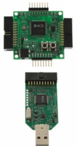
The XMOS XK-1A microcontroller development board was used as the main embedded controller for this project. The XMOS XK-1A is a low cost development board which is based on a single XS-L1 device. It consists of a single XCore, which comprises an event-driven multi-threaded processor with general purpose I/O pins and 64 KBytes of on-chip RAM. In addition, the device consists of two XSYS 20-way IDC headers (one female and one male), an SPI interface to FLASH memory, a 20 MHz crystal oscillator, and two expansion areas with 12 I/O pins each [42]. Programming the device can be done through the use of a JTAG device known as an XTAG that has a USB interface. The device can be programmed with XC programming language in an Eclipse-based environment known as XMOS Development Environment (XDE), which is supplied by XMOS. Figure 3.1 shows the XK-1A microcontroller development board and XTAG interface.

XMOS technology was chosen for the development of the miniature UGV due to its numerous advantages over current processors used in intelligent, unmanned autonomous systems. The XMOS microcontroller utilizes an event-driven parallel processor, which unifies high-level processing with low-level control to overcome the complexity of han-dling multiple I/O streams while simultaneously performing complex computational tasks required for intelligent behavior [43]. However, the XMOS device also contains a number of disadvantages as well. For example, the small amount of memory that the device carries makes it not very applicable for vision-based control applications.

3.2.2

Servo Motors

Another critical component to the vehicle design is the servo motor. The miniature UGV consists of two standard analog servo motors. The servo motors were modified to be con-tinuous rotation so that they could be used for the unicycle-type drive mechanism. The

Figure 3.1: XMOS XK-1A Development Board and XTAG

reason for this was primarily due to the reduced cost of standard servo motors over tra-ditional continuous rotation motors. The servo motor used in the miniature UGV is the HK15138 Standard Analog Servo motor from Hobby King (see Figure 3.2). This servo motor can be easily operated with a voltage of 4.8 V to 6 V. The motor provides a torque of 3.8 kg to 4.3 kg and a maximum speed of 0.21 seconds per 60 degrees to 0.17 seconds per 60 degrees.

Figure 3.2: Hobby King HK15138 Standard Analog Servo Motor

3.3

First Generation Vehicle Design

The first generation miniature UGV design was developed using SolidWorks 3D CAD de-sign software. A basic drawing of the first dede-sign revision can be seen in Figure 3.3. A simple prototype, as seen in Figure 3.4, was designed in the University of Denver’s Un-manned Systems Research Institute and manufactured in the University of Denver’s ma-chine shop. The chassis was designed in SolidWorks and cut with aluminum to assemble the unicycle-type drive mechanism with two continuous rotation servo motors and a ball castor for initial proof of concept. This first vehicle design measured at 75mm by 142mm and contained only holes for the two servo motors and standoffs for the XMOS microcon-troller.

The prototype above in Figure 3.4 was used to perform manual motion control of the vehicle using radio control both directly through a radio receiver and subsequently through an interface with the XMOS XK-1A microcontroller development board. Following the verification of manual motion control, the vehicle design was then modified in SolidWorks to be manufactured using 3D printing. In particular, the design was made to be more durable for the plastic material it was to be printed with. As a result, the overall thickness of the 3D printed chassis was increased to 3 mm due to the constraints of the 3D printer that

Figure 3.3: Vehicle Drawing of Miniature UGV, rev. 1

Figure 3.4: Initial Prototype of First Generation Miniature UGV

was used to develop it. Additionally, the vehicle chassis was designed to accommodate the size of a standard analog servo motor. This allows for any brand of standard servo motor to be installed on the vehicle quite easily. The servo motors onboard the miniature UGV can

be driven with pulse-width modulation (PWM) signals. These signals vary in duty cycle between 1.0 ms and 2.0 ms and are used as the inputs to the system to control the velocity of the wheels through software implemented on the XMOS microcontroller.

The first generation SolidWorks design can be seen in Figure 3.5. The resulting printed chassis can be seen in Figures 3.6 and 3.7 and was used to assemble the first generation of the miniature UGV that contained all other necessary components.

Figure 3.5: Miniature UGV SolidWorks Design, Version 1

Figure 3.7: 3D Printed Chassis and Bumper

The fully assembled miniature UGV can be seen in Figure 3.8. The vehicle consists of a XMOS XK-1A microcontroller board, breakout printed circuit board, 5 V battery pack, continuous rotation servo motors with wheels, tactile bumper sensors, and compass module. A total of 15 vehicles were initially assembled at the University of Denver’s Unmanned Systems Research Institute and can be seen in Figure 3.9. This initial group of vehicles was manufactured and used for the University of Denver’s Embedded Systems Programming Course, ENCE 4800. Applications performed in the course involved the vehicle using Breadth First Search and A* Star Search algorithms to navigate through a maze. Additionally, the vehicle was interfaced with tactile bumper sensors and a compass to perform simple navigational and obstacle avoidance tasks.

Several faults in the first generation vehicle design were discovered over the course of the vehicle’s extensive use in the University of Denver’s Embedded Systems Programming class during Spring 2012. The most immediate fault was easily found in the vehicle’s bumper mechanism. The initial bumper system was attached to the vehicle with epoxy that was applied to two tactile bumper switch sensors made from aluminum. This simple design

Figure 3.8: Fully Assembled First Generation Vehicle

Figure 3.9: Initial Fleet of 3D Printed Miniature UGV’s

was found to lack durability when the vehicle experienced a collision. Other faults with the design related to the lack of space on the vehicle for additional sensors.

3.4

Second Generation Vehicle Design

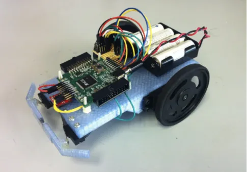
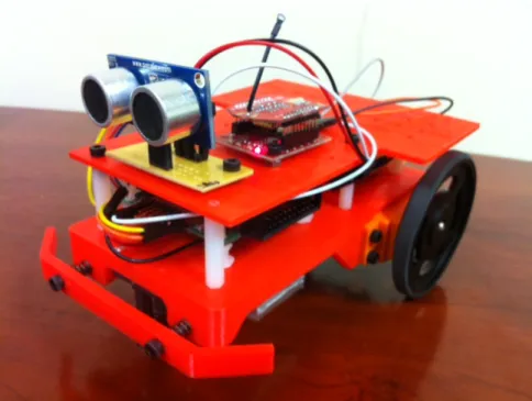
The second generation miniature UGV design, seen in Figure 3.10, makes several improve-ments over the first generation. The two major revisions involved the vehicle chassis and bumper system. These revisions were designed to improve the faults discovered with the first generation vehicle design as well as reduce overall cost of the vehicle.

Figure 3.10: Assembled Second Generation Vehicle

3.4.1

Chassis Design

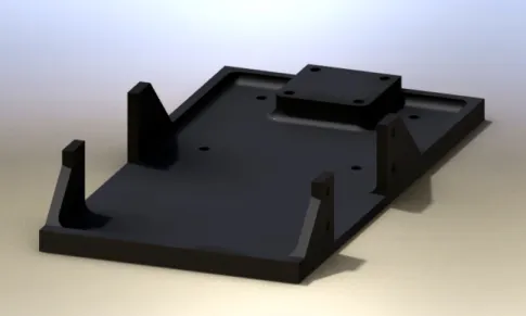
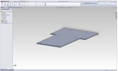
The main improvement on the second generation vehicle was a redesign of the vehicle’s chassis to incorporate a top plate to allow for more space on the vehicle as seen in Figures 3.13 and 3.14. This involved adding additional standoffs to the main chassis design in Solidworks and designing a separate top plate to be placed on them. Also, the mounting location of the servo motors was moved back to create more room underneath the vehicle for a battery pack as can be seen in Figure 3.15.

Figure 3.11: Second Generation Vehicle with Laser Range Finder

The second generation chassis dimensions are 75 mm by 142 mm, which is the same as the previous generation vehicle. There was no significant increase to the second generation chassis due to the size constraints on the 3D printer that was used to develop it. The standoff holes are spaced in a 54 mm by 122 mm rectangular configuration along the length of the vehicle, and the standoffs lift the vehicle top plate 25 mm above the chassis. This additional height gives the top plate clearance over the vehicle’s wheels so that there is additional space for many different applications.

Overall, the second generation vehicle was designed to accommodate for a number of different sensors and actuators for different research applications. Figures 3.11 and 3.12 above show two different configurations of the second generation vehicle design for different types of sensors. These particular vehicles are the ones primarily used in this work.

Figure 3.14: Chassis Top Plate

Figure 3.15: Chassis Re-Design with Adjusted Servo Mount

3.4.2

Bumper Design

Additionally, a new bumper system was designed for the vehicle to add durability for colli-sion detection during forward motion. The main problem with the original bumper design was that it was not durable enough to withstand a large number of collisions during regu-lar use. This was primarily due to the original bumper being attached to aluminum tactile

bumper switch sensors with epoxy. Figure 3.16 shows the original bumper design, which could easily be detached from the vehicle with minimal force when small collisions oc-curred. As a result of the poor performance of the original bumpers, there was a desire on the second generation vehicle design to incorporate a more durable bumper system that could withstand all collisions. The redesigned bumper system can be seen in Figures 3.17 and 3.18.

Figure 3.16: Original Bumper Design

Figure 3.17: Second Generation Bumper Design

The second generation bumper system design is comprised of a 3 mm thick 3D printed plastic bumper that was designed in Solidworks. This bumper design differed from the orig-inal with two M3 screw holes that were used to attach the bumper to the vehicle with two 20 mm long M3 screws. Using 9.4 mm compression springs, the M3 screws are mounted on the front of the vehicle so that compression may occur when the vehicle experiences front side collisions. When the bumper compresses, a tactile bumper switch sensor is com-pressed sending the signal of a collision to the microcontroller.

Figure 3.18: Second Generation Bumper Design (angled view)

3.4.3

Power Budget

For the particular application in this project, it is necessary for a power source to be chosen that can allow the vehicle to operate normally for an acceptable amount of time. It is desired that a battery be chosen so that the vehicle may operate for a long enough period in order to perform experiments in a number of different applications. Batteries typically used in robotics include alkaline, fuel cell, lead acid, lithium, NiCad, and NiMH. The battery that was available and chosen for this project was a 11.1 V Lithium-Polymer Battery with 730 mAh. A power budget was made to determine the amount of battery life available with the vehicle for this project.

The power budget presented in Table 3.4 is useful in determining the total power re-quired to operate the mobile robot system. This table shows the maximum current draw of all sensors and actuators onboard the vehicle designed above. The total current of the

Component Voltage Maximum Current Draw XMOS XK-1A 5 V 200 mA Standard Servo 5 V 200 mA Standard Servo 5 V 200 mA Hokuyo URG-04LX 5 V 800 mA Honeywell Compass 3.3 V 10 mA Data Logger 3.3 V 6 mA

Roving Networks WiFly 3.3 V 180 mA

Table 3.4: Vehicle Power Budget

system with all components is 1596 mA, or 1.596 Amps. This information allows us to find the approximately battery life of the vehicle, which is approximately 27 minutes. This means that with all components drawing maximum current, the vehicle’s battery would only last this much time.

3.5

Cost Analysis

A small unmanned ground vehicle was designed with focus on low cost and simplicity in design. As discussed above, many small mobile robot systems exist, which are relatively high in cost and lack components or space required for swarm behavior research. Table 3.5 shows the overall cost of parts that are required to build the small UGV designed in this project.

As can be seen from the vehicle parts list in Table 3.5, the total cost to build one of the second generation small UGV’s discussed in this chapter is $32.01. It is important to note that this vehicle cost does not include the cost of the XMOS microcontroller, which is sold by XMOS for $59.00. This total cost, excluding the XMOS microcontroller, is significantly less than the other existing mobile robot systems described in Table 3.1. It is also important to note that some of these systems do not include a microcontroller. Also, the systems that do contain a microcontroller have one that is significantly cheaper than the

Part Count/Vehicle Price/Unit ($) Total

Standard Servo 2 3.12 6.24

Wheel w/ Band 2 3.5 7.00

Ball Caster Kit 0.5 6.00 3.00

Vehicle Material 1 2.66 2.66 Jumper Wires 1 2.50 2.50 AA Battery Pack 1 1.19 1.19 AA Battery 2 0.68 1.36 25 mm M3 Standoff 4 0.45 1.80 8 mm M3 Screws 12 0.04 0.48 20 mm M3 Screws 2 0.06 0.12 M3 Nuts 2 0.01 0.02 9.4 mm Spring 2 2.07 4.14 PCB Standoff 1 1.50 1.50 $32.01 Table 3.5: Vehicle Parts List

overall cost of the system. The vehicle created in this project is relatively simple in design and is significantly cheaper than other existing small mobile robot systems.

It is also possible to reduce the cost of the vehicle further by purchasing components in bulk and utilizing cheaper materials. For example, the ball caster kit used onboard the vehicle cost $6.00. However, if this component were to be ordered in a large quantity for the manufacturing of many vehicles, the cost could be reduced to $5.63. This applies to many of the components that are listed in Table 3.5 above.

Additionally, as mentioned above, some of the existing systems listed in Table 3.1 in-clude microcontrollers with the mobile robot. However, the cost of these microcontrollers is significantly cheaper than a microcontroller such as the XMOS XK-1A used in this project. Additionally, these other microcontrollers do not necessarily have the ability to operate and perform multiple simultaneous tasks that are required for autonomous unmanned ground systems. For example, the 3pi mobile robot system from Pololu Robotics includes an ATmega328P microcontroller in its $99.95 price. The ATmega328P microcontroller can be purchased for as little as $2.24 from sources such as Mouser Electronics whereas the

XMOS XK-1A costs $59.00 from XMOS. This shows that the cost of these existing sys-tems excluding any microcontroller or processor is significantly more expensive than the cost to produce the vehicle used in this project.

Chapter 4

Vehicle Kinematics and Control

This chapter discusses the modeling and control for the miniature UGV design of unicycle-type presented in Chapter 3. The notion of nonholonomic systems is presented, and the kinematic model of the vehicle is derived. Motion control is applied using feedback lin-earization techniques, and control is further developed for application in formations utiliz-ing the Leader-Follower formation method. The followutiliz-ing text and figures presented in this chapter are adopted from [1] and [44].

4.1

Kinematic Model

The unicycle mobile robot is a vehicle with a simple drive mechanism that is commonly used for indoor applications in current robotics and controls research. Figure 4.1 shows the schematic of a unicycle type vehicle. This type of mobile robot is the primary vehicle used in this work and was the basis for the miniature UGV design presented in Chapter 3. The drive mechanism uses two independent motors, each of which power one of the vehicle’s wheels. The kinematic inputs that drive the vehicle as well as affect its speed and direction of motion are the two individual wheel velocities. However, it is convenient in most

ap-plications to choose the linear and angular velocity of the vehicle as a whole as the inputs to the kinematic model. The reason for this is that most commercially available mobile robots, including those seen in Figure 1.1, utilize a low level controller which controls both the linear and angular velocities of the vehicle.

164 6 Mobile Robots

Fig. 6.1 A Hilare mobile robot

wheels. Thus, the actual kinematic inputs that drive the robot and affect its speed

and direction of motion are the two wheel speeds. With this in mind, at first glance

it seems intuitive to write the kinematic equations of motion of a Hilare mobile

robot in terms of these speeds. However, on most commercial mobile robots, there

exists a low-level controller that controls the linear and angular velocity of the robot.

Therefore, for application purposes, it is more convenient to choose the linear and

angular velocity of the mobile robot as the inputs of the kinematic model. When a

control law is found later based on this model, it can be more easily applied using

the development packages available for commercial robots.

Now, consider the Hilare-type mobile robot shown in Fig. 6.1. Assume that the

robot motion is reasonably slow such that the longitudinal traction and lateral force

exerted on the robot’s tires do not exceed the maximum static friction between the

tires and the floor in the longitudinal and lateral directions. In other words, assume

that no-slip happens between the robot’s tire and the floor during the whole motion

of the robot.

The first direct result of this assumption is that the velocities of the center of

the robot’s wheels do not have any lateral components. As a consequence, one can

assume that the velocity of point (

x

,

x

center of the wheels, does not have any lateral component and is parallel with the

wheel planes. The second result of the no-slip assumption is that one can relate the

velocity of point (

x

,

x

), the midpoint of the line attaching the center of the wheels,

to the rotational velocity of the wheels.

Before writing the kinematic equations of motion for the robot, one has to define

the configuration variables of the robot. Let the coordinates of point (

x

,

x

) define

the global position of the robot with respect to the inertial coordinate system

x

−

x

.

Consider a line that is perpendicular to the wheel axis and goes through the point

Figure 4.1: Schematic of Unicycle-type Mobile Robot [1]

In Figure 4.1, it is assumed that there is no wheel slipping between the vehicle’s wheels and the ground surface while the vehicle is in motion. In other words, it is assumed that the vehicle is moving at a relatively slow speed such that the lateral force and longitudinal traction exerted on the wheels does not exceed the maximum static friction between the wheels and the ground surface in both the lateral and longitudinal directions. As a result of this assumption, the individual velocities of the wheels do not have any lateral components. This means that one can assume that the velocity of the midpoint between the two wheels at (x1, x2) does not contain any lateral component and is therefore parallel with the plane of the wheels. This constraint with respect to no lateral velocity with the wheels is known

as the nonholonomic constraint. One can also relate the center point of the wheels (x1,x2) with rotational velocity of the wheels.

The configuration variables of the unicycle-type vehicle must be defined before the kinematic equations can be defined. Let the coordinates of the point (x1,x2) be the global position of the vehicle with respect to the inertial coordinate systemx1andx2. The line in Figure 4.1 that is perpendicular to the wheel axis and goes through the midpoint between the wheels (x1, x2) can be considered an orientation reference for the vehicle. The angle that this line makes with the positive x1 axis is called θ and represents the orientation of the vehicle. Equation 4.1 shows the kinematic equations of motion for the unicycle-type nonholonomic vehicle in matrix form.

      ˙ x1 ˙ x2 ˙ θ       =       cosθ 0 sinθ 0 0 1          v ω    (4.1)

As can be seen from the kinematic model, the three variables that define the geometric configuration of the robot arex1,x2, andθ. In addition to the no wheel slip assumption, it can also be assumed that the vehicle at center wheel axis point (x1,x2) moves with a linear velocity ofv and an angular velocity ofω. These velocities are assumed to be the system inputs and are presented in an input vector in the kinematic model. Equation 4.1 can be numerically integrated to predict the motion of the robot if the input vector is known as a function of time. Different inputs may also be chosen for the system such as rotational velocities of the wheels or the difference between linear velocities of the wheels, however, the linear velocity v and angular velocity ω of the vehicle as a whole are chosen in this work due to the simplicity and well known documentation of this method.

4.1.1

Discrete Time Kinematic Model and Control

The motion tasks performed in this project are implemented on the XMOS processor in discrete time. Therefore, it is necessary to discretize the kinematic model shown in 4.1 and 4.3. If we consider a time interval of ∆t, a sampling instant ofk, and apply Euler’s approximation to the kinematic model of equations in 4.3, we can obtain the following discrete-time model for the unicycle type vehicle shown in 4.2.

x1(k+ 1) =x1(k) +v(k) cos(θ(k))∆t

x2(k+ 1) =x2(k) +v(k) sin(θ(k))∆t

θ(k+ 1) =θ(k) +ω(k)∆t

(4.2)

Equation 4.2 shows the discretization of the unicycle kinematic equations of motion which is implemented on the vehicle in this project. The control inputs of this system of equations are v(k) and ω(k), which are velocity and angular heading rate of change, respectively. These control inputs are constant over the time interval∆t. In this particular work, predefined trajectories on a finite time horizon are implemented on the vehicle by choosing pairs ofv andω. Each pair of linear and angular velocities is executed on the vehicle and held for a predetermined amount of time. This predetermined amount of time,

∆t, can vary with each command and can be chosen such that the vehicle traverses along the desired trajectory.

With regards to the leader-follower formation control implemented in this project, the trajectory, or array of linear and angular velocity commands of the follower vehicles, is produced by a PID control task in software based on sensor feedback. This task is per-formed over a given time horizon, in this particular case the length of the leader vehicle’s trajectory. Each time interval∆thas a constant linear velocityv and angular velocityω

as-sociated with it. The vehicle path becomes a smooth collection of arcs which demonstrates how the unicycle-type vehicle is unable to travel precisely along a straight trajectory. In this case, command durations ∆t are100 ms, which was determined by the frequency of the laser range finder’s sweep. This specific result is discussed in more detail in Chapter 5.

4.2

Trajectory Tracking Control

A common topic in robotics and controls research is trajectory tracking for the nonholo-nomic unicycle type vehicle. A trajectory tracking controller is useful for robots to be able to follow a planned trajectory. In this section, kinematic trajectory tracking control is presented based on the unicycle-type vehicle. This topic is discussed further in [45] and [1]. The control inputs for the unicycle-type vehicle are assumed to bev andωas defined above in the previous section. Once again the kinematic equations of motion are written in Equation 4.3. ˙ x1 =vcosθ ˙ x2 =vsinθ ˙ θ =ω (4.3)

If we assume that the desired trajectory of the vehicle is in the inertial coordinate system and can be defined as functions of time, then two position components xd

1(t) and xd2(t) can be selected as the vehicle’s desired positions. The desired velocity components of the vehicle can be derived by differentiating these position components. As a result, we getxd˙

1(t)andxd2˙(t)through differentiation. These velocities are functions of time, which means that the vehicle must follow a desired speed that has been pre-defined. The desired

positions of the vehicle,xd

1(t)andxd2(t), contain information about the desired velocity as well as the geometry of the desired path.

Once the desired velocity components are obtained inxd˙

1(t)andxd2˙(t), the desired head-ing or orientation of the vehicle must be found. Due to the nonholonomic constraint of the unicycle-type vehicle, there are limitations in the desired orientation that can be selected. The desired orientation must adhere to the vehicle’s lateral no-slip condition. In other words, the vehicle has a zero lateral velocity at all times. The nonholonomic constraint of this particular type of vehicle can be conveyed in Equation 4.4. This constraint is well known in literature on control applications of mobile robots or unmanned ground vehicles.

˙

xr

2 =−x˙1sinθ+ ˙x2cosθ= 0 (4.4)

Once the desired velocity components are obtained, the desired heading or orientation can be derived. This is shown below in Equation 4.5.

θd(t) = arctan ˙ xd 2(t) ˙ xd 1(t) (4.5) A common technique utilized in current research literature is to reduced the system to chained form. A new set of configuration variables can be found that can simplify the kinematic model of the unicycle-type mobile robot. If we observe the kinematic model shown in Equation 4.1, the chained form configuration variables can be written as those seen in Equation 4.6.

z1 =x1

z2 = tanθ

z3 =x2

The chained form is well known in literature pertaining to mobile robots and unmanned ground systems. The chained form control inputs to the kinematic model are shown in Equation 4.7.

u1 =vcosθ

u2 =ω(1 + tan2θ)

(4.7)

If we apply these new variables to the original kinematic equations shown in Equation 4.3, then we get a new chained form for the kinematic equations of motion for the unicycle-type vehicle. This chained form can be seen in Equation 4.8. This chain form method can be extended for different vehicle types with different drive mechanisms and configuration variables as well.

z1 =u1

z2 =u2

z3 =z2u1

(4.8)

Once we have the chained form kinematic model, we can find the desired trajectory for the variables shown in Equation 4.6. This is done by substituting the desired position com-ponents into Equation 4.6. The control inputs can then be found by substituting Equation 4.6 into Equation 4.8. The new desired trajectory can be seen in Equation 4.9.

z₁d(t) =xd₁(t) z₂d(t) = ˙ xd 2(t) ˙ xd 1(t) z₃d(t) =xd₂(t) (4.9)

It is desired to control the chained form kinematic equations shown in Equation 4.8 to follow the new trajectory shown in Equation 4.9. The error from this application can be derived simply by subtracting the desired configuration variables from the actual configu-ration variables. The error equations are nonlinear and can be seen in Equation 4.10 where

˜

zi =zi−zidfori= 1,2,3andu˜i =ui−udi fori= 1,2.

˙˜ z1 = ˜u1 ˙˜ z2 = ˜u2 ˙˜ z3 =z2du˜1+ ˜z2ud1+ ˜z2u˜1 (4.10)

The first step that must be taken is to linearize the nonlinear system of equations. A common technique in current research practices with almost all nonlinear systems is to use the method of feedback linearization. The general idea of this method is to algebraically transform nonlinear systems into linear ones so that linear control techniques can be ap-plied. This method is chosen over the other common method of linearization, known as Jacobian linearization, which for the unicycle kinematic model results in an unstable sys-tem [45]. To do this,z˜2u˜1 is neglected and the time-variant feedback control law shown in Equation 4.11 is assumed wherek1,k2, andk3 are constant controller gains.

   ˜ u1 ˜ u2   =    k1 0 0 0 k2 k3/ud1          ˜ z1 ˜ z2 ˜ z3       (4.11)

The control law in Equation 4.11 is then applied to the linear state error equations shown in Equation 4.10.       ˙˜ z1 ˙˜ z2 ˙˜ z3       =       k1 0 0 0 k2 k3/ud1 k1z1d ud1 0       (4.12)

This gives us the linear time variant closed loop system, which can be seen below in Equation 4.12. The linear time variant closed loop system in Equation 4.12 is time dependent, however, its characteristic equation is not time dependent. Therefore, one can select controller gains such for the linearized system. The controller gains suggested in [1] arek1 = −λ1, k2 = −2λ2, and k3 = −(λ22 +λ23) whereλ1 andλ2 are positive constant values. With these selected gains, the closed loop system becomes asymptotically stable. As a result, the poles of the system become−λ1,−λ2+iλ3, and−λ2−iλ3.

The new inputs of the system can then be calculated from the control law in Equation 4.11 by using the errors in Equation 4.10 with respect to the desired trajectory. Using the chain form control inputs in Equation 4.7, the linear and angular velocities of the unicycle-type vehicle can be found. These are shown in Equation 4.13.

v = u˜1+u d 1 cosθ ω = u˜2+u d 2 1 + tan2_θ (4.13)

Tracking control can then be performed for a predefined trajectory, for example a piece-wise linear path or a sinusoidal path. To do this, the desired position and velocity compo-nents must be derived as functions of time according to the path definition. Then, any errors between the desired configuration values and current configuration values can be computed using Equation 4.10. The computed errors can then be used in Equation 4.11 for the linearized feedback control law. Using these computed values, the linear and velocity commandsv andωcan be found using Equation 4.13.

4.3

Leader-Follower Formation Control

An ongoing research area in controls and robotics is the study of multi-vehicle systems and swarming, where it is desired to control a group of robots for a particular application. This type of system holds several advantages as discussed in Chapter 1, and several tech-niques currently exist in order to address control issues with multiple vehicles moving in formation. These techniques are discussed in more detail in Chapter 2.

In this section, the leader-follower approach is analyzed and discussed for a particular application that utilizes decentralized control. It is assumed that the overall motion of the formation is known to a single vehicle who is designated as the leader, and that all other vehicles, or followers, are aware of the relative position of vehicles directly ahead of them through some type of inter-vehicle communication or vision. The leader follows a given pre-defined trajectory while the follower is controlled by local control laws. The decen-tralized control for each vehicle is derived from the dynamics of its relative position to the leader. The following is based on the concepts presented in [5] and [1] where a controller is designed that controls the relative distance and heading of the follower relative to the leader vehicle. It is important to know that additional leader-follower control designs exist that involve a follower vehicle that maintains its position in the formation by keeping

spec-ified distance with multiple leader vehicles. The work presented in this thesis demonstrates leader-follower formation control for a single leader vehicle.

The leader-follower formation involving two vehicles, a leader and a follower, is shown in Figure 4.2. The distance between the center of the wheel axis of the leader and the center control pointpon the follower isl12. In order to maintain the vehicle formation, the follower vehicle must maintain a desired distance ld₁₂ and desired angle αd₁₂ with respect to the leader vehicle. To do this, a relation of inputs and outputs is required between the system inputs, v2 and ω2, and the control outputs, ld12 and αd12. This type of control is typically called ”l−α” control in literature.

6.4 Formation Control for Hilare Mobile Robots 183

It is also assumed that each robot is aware of the relative position of other robots

that are immediately adjacent to it via communication or some kind of vision. While

the lead robot follows the given trajectory, the rest of the robots in the formation are

controlled by local (decentralized) control laws. The control law for each robot in

the formation is derived based on the dynamics of its relative postion with respect

to the neighboring robots in the formation. This type of decentralized control law

has the advantage of providing easily computable, real-time feedback control, with

provable performance for the entire system.

6.4.1 Geometrical Leader-Follower Formation Schemes

Based on the methodology introduced in [22], in this section, two schemes for

feed-back control of the relative distance of the robots within a formation are described.

The first scheme is a controller that controls the relative distance and view angle of

one robot (the local follower) relative to one neighboring robot (the local leader).

This control scheme is used in situations where each robot has one leader, for

exam-ple, where robots march in a single file or at an edge of a 2D formation geometry.

The second scheme is a controller that allows a robot (a local follower) to maintain

its position in the formation by keeping specified distances with two neighboring

robots (local leaders).

6.4.2 Design of the l –

α

Controller

Two neighboring robots in the formation are shown in Fig. 6.13. The distance of the

center of axle of robot 1 and the control point,

p, of robot 2 is

l

. The control point

is on the longitudinal axis of robot 2 and has a distance

d

from the center of the axle

Fig. 6.13 Thel–αcontrol scheme

Figure 4.2: Schematic of Leader-Follower Formation [1]

The first step to this method is to perform a kinematic analysis of the relative motion of the vehicles. It is assumed that there is a moving coordinate system with an origin at the center of the wheel axis of the leader vehicle that rotates with the vectorl12, which is the distance that the follower vehicle sees with respect to the leader. It is also assumed that there are two points,p1 andp2, which are connected to the coordinate frame on the leader vehicle and follower vehicle, respectively. When looking at the follower vehicle from point