SURFACE
SURFACE
Dissertations - ALL SURFACE
December 2019
Copula-based Multimodal Data Fusion for Inference with
Copula-based Multimodal Data Fusion for Inference with
Dependent Observations
Dependent Observations
Shan ZhangSyracuse University
Follow this and additional works at: https://surface.syr.edu/etd
Part of the Engineering Commons
Recommended Citation Recommended Citation
Zhang, Shan, "Copula-based Multimodal Data Fusion for Inference with Dependent Observations" (2019). Dissertations - ALL. 1142.
https://surface.syr.edu/etd/1142
This Dissertation is brought to you for free and open access by the SURFACE at SURFACE. It has been accepted for inclusion in Dissertations - ALL by an authorized administrator of SURFACE. For more information, please contact
Fusing heterogeneous data from multiple modalities for inference problems has been an at-tractive and important topic in recent years. There are several challenges in multi-modal fusion, such as data heterogeneity and data correlation. In this dissertation, we investigate inference problems with heterogeneous modalities by taking into account nonlinear cross-modal depen-dence. We apply copula based methodology to characterize this dependepen-dence.
In distributed detection, the goal often is to minimize the probability of detection error at the fusion center (FC) based on a fixed number of observations collected by the sensors. We design optimal detection algorithms at the FC using a regular vine copula based fusion rule. Regular vine copula is an extremely flexible and powerful graphical model used to characterize complex dependence among multiple modalities. The proposed approaches are theoretically justified and are computationally efficient for sensor networks with a large number of sensors. With heterogeneous streaming data, the fusion methods applied for processing data streams should be fast enough to keep up with the high arrival rates of incoming data, and meanwhile provide solutions for inference problems (detection, classification, or estimation) with high ac-curacy. We propose a novel parallel platform, C-Storm (Copula-based Storm), by marrying copula-based dependence modeling for highly accurate inference and a highly-regarded par-allel computing platform Storm for fast stream data processing. The efficacy of C-Storm is demonstrated.
In this thesis, we consider not only decision level fusion but also fusion with heterogeneous high-level features. We investigate a supervised classification problem by fusing dependent high-level features extracted from multiple deep neural network (DNN) classifiers. We employ regular vine copula to fuse these high-level features. The efficacy of the combination of model-based method and deep learning is demonstrated.
tial detection problem withrandom-sample-size. The aim of the distributed sequential detec-tion problem in a non-Bayesian framework is to minimize the average detecdetec-tion time while satisfying the pre-specified constraints on probabilities of false alarm and miss detection. We design local memory-less truncated sequential tests and propose a copula based sequential test at the FC. We show that by suitably designing the local thresholds and the truncation window, the local probabilities of false alarm and miss detection of the proposed local decision rules satisfy the pre-specified error probabilities. Also, we show the asymptotic optimality and time efficiency of the proposed distributed sequential scheme.
In large scale sensors networks, we consider a collaborative distributed estimation prob-lem with statistically dependent sensor observations, where there is no FC. To achieve greater sensor transmission and estimation efficiencies, we propose a two-step cluster-based collabo-rative distributed estimation scheme. In the first step, sensors form dependence driven clusters such that sensors in the same cluster are dependent while sensors from different clusters are independent, and perform copula-based maximum a posteriori probability (MAP) estimation via intra-cluster collaboration. In the second step, the estimates generated in the first step are shared via inter-cluster collaboration to reach an average consensus. The efficacy of the proposed scheme is justified.
INFERENCE WITH DEPENDENT OBSERVATIONS
By
Shan Zhang
B.S., University of Science & Technology Beijing, China, 2014
DISSERTATION
Submitted in partial fulfillment of the requirements for the degree of Doctor of Philosophy in Electrical and Computer Engineering
Syracuse University December 2019
First and foremost, I would like to express my deepest gratitude and sincere thanks to my advisor, Prof. Pramod K. Varshney, for his guidance, support and encouragement. I have been amazingly fortunate to have him during my doctoral study. He gave me the freedom to explore on my own, and at the same time guidance to recover when my steps faltered. He has been influencing me with his enthusiasm towards research as well as life, and will keep guiding me in the future.
Besides my advisor, I would like to thank Mrs. Varshney for her kindness, support and all the home-cooked meals. She is like a mother to me. She is a very strong and inspiring woman. She made me understand the true meaning of love. I have learned a lot from her, and will miss her very much.
I would like to thank the rest of my thesis committee: Prof. Biao Chen, Prof. Lixin Shen, Prof. Mustafa C. Gursoy, Prof. Chilukuri K. Mohan and Prof. Reza Zafarani for their insightful comments and suggestions. Dr. Lakshmi N. Theagarajan and Dr. Sora Choi have provided technical support for part of the work in this thesis.
Also, I would like to thank all my fellow labmates in the Sensor Fusion Laboratory for their constant support in my research and life: Pranay Sharma, Prashant Khan-duri, Swatantra Kafle, Saikiran Bulusu, Qunwei Li, Baocheng Geng, Quan Chen and Nandan Sriranga. Also, I would like to take this opportunity to thank Dr. Sijia Liu, Dr. Aditya Vempaty, Prof. Vinod Sharma and Prof. Jian Tang for their patient guidance and support. Especially, I am very grateful to have Dr. Nianxia Cao, Dr. Hao He, Dr. Fangrong Peng, my friends Mingyue Wang and Qianyun Wang during my doctoral
Most importantly, none of this would have been possible without the love and constant encouragement of my parents, my brother and my husband. I would like to thank them for always being there cheering me up and standing by me through the good times and bad.
Acknowledgments v
List of Tables xi
List of Figures xiii
1 Introduction 1
1.1 Background . . . 2
1.1.1 Copula Theory . . . 3
1.1.2 Summary of Some Multivariate Copula Functions . . . 4
1.1.3 Copulas and Measures of Dependence . . . 5
1.1.4 Regular Vine Copula . . . 6
1.1.5 Array Representation of Regular Vine . . . 10
1.2 Literature Review . . . 11
1.2.1 Linear Dependence: Covariance Matrix . . . 12
1.2.2 Nonlinear Dependence: Nonparametric Approach . . . 13
1.2.3 Nonlinear Dependence: Copula-based Approach . . . 14
1.3 Main Contributions and Organization . . . 16
1.4 Bibliographic Note . . . 18
2 Distributed Detection Based on Regular Vine Copulas 20 2.1 Motivation . . . 20
2.3 R-Vine Copula Based Fusion of Multiple Statistically Dependent Decisions . . 24
2.3.1 Optimal Test Statistic . . . 24
2.3.2 R-Vine Copula Based Dependence Modeling . . . 28
2.3.3 Model Selection and Estimation . . . 29
2.4 Efficient R-Vine Copula Based Fusion with Statistical Dependent Decisions . . 31
2.5 Simulation Results . . . 34
2.6 Summary . . . 42
3 Copula based Distributed Parallel Computing Platform 43 3.1 Motivation . . . 43
3.2 Storm . . . 44
3.3 Design of C-Storm . . . 45
3.3.1 Architecture of C-Storm . . . 45
3.3.2 Copula-based Dependence Modeling . . . 48
3.4 Simulation Results . . . 50
3.4.1 Fusion Application and Experimental Setup . . . 50
3.4.2 Experimental Results and Analysis . . . 52
3.5 Summary . . . 55
4 Distributed Classification with Dependent Features 56 4.1 Motivation . . . 56
4.2 Problem Formulation . . . 58
4.3 R-Vine Copula Based Fusion of Multiple Deep Neural Networks . . . 60
4.3.1 R-Vine copula Models . . . 61
4.3.2 Estimation of Optimal R-Vine copula . . . 61
4.4 Simulation Results . . . 62
4.4.2 Classification Accuracy . . . 64
4.5 Summary . . . 66
5 Distributed Sequential Detection with Dependent Observations 68 5.1 Motivation . . . 68
5.2 Problem Formulation . . . 69
5.3 Centralized Copula-based Sequential Probability Ratio Test . . . 72
5.4 Distributed Copula-based Sequential Probability Ratio Test . . . 77
5.4.1 Local Sensor Detection Rule . . . 78
5.4.2 Derivation of the Fusion Rule . . . 81
5.5 Simulation Results . . . 83
5.6 Summary . . . 90
6 Distributed Estimation in Large Scale Wireless Sensor Networks via A Two-Step Cluster-based Approach 92 6.1 Motivation . . . 92
6.2 Problem Formulation . . . 93
6.3 Two-Step Dependence Driven Collaborative Distributed Estimation . . . 97
6.3.1 Assumptions and Dissimilarity Measure Definitions . . . 98
6.3.2 Dependence Driven Clustering Process . . . 99
6.3.3 Copula Based MAP . . . 100
6.3.4 Cluster Based Consensus Scheme . . . 103
6.4 Sensor Selection Based Two-Step Dependence Driven Collaborative Distributed Estimation . . . 105
6.5 Simulation Results . . . 108
6.6 Summary . . . 116
7.1 Summary . . . 118
7.2 Future Directions . . . 121
Appendix 123 A Aut in Log Test Statictics (2.6) . . . 123
B Proof of Theorem 2.1 . . . 124 C Proof of Theorem 5.1 . . . 125 D Proof of Theorem 5.2 . . . 128 E Proof of Theorem 5.3 . . . 129 F Proof of Theorem 6.1 . . . 130 G Proof of Theorem 6.2 . . . 130 References 135 x
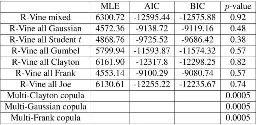
1.1 Archimedean copula functions. . . 5 2.1 The performance of R-Vine classes and standard multivariate copulas. . . 37 4.1 STISEN: F1 scores for Watch-DNN, Phone-DNN, Fully-connected layer
fu-sion, Data-level fufu-sion, R-Vine copula fusion. . . 64 4.2 ANGUITA:F1scores for Accelerometer-DNN, Gyroscope-DNN, Fully-connected
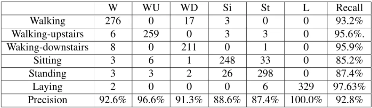
layer fusion, Data-level fusion, R-Vine copula fusion. . . 64 4.3 STISEN: Confusion matrix for R-Vine copula based fusion. . . 66 4.4 ANGUITA: Confusion matrix for R-Vine copula based fusion. . . 66
5.1 Known copula: EstimatedPF and PM withα = 0.01, L = 3 for centralized
sequential scheme and Case1. . . 85 5.2 Known copula: EstimatedPF and PM withβ = 0.01, L = 3 for centralized
sequential scheme and Case1. . . 85 5.3 Average p values for the estimation of underlying dependence using R-Vine
copula model with different number of sensors. . . 86 5.4 Averagepvalues for the estimation of underlying dependence using different
multivariate copula models withL= 3. . . 87 5.5 Unknown copula: EstimatedPF,PM andE[T]withα=β = 0.01and SNR=
−6dB. . . 89
−9dB. . . 89 5.7 Unknown copula: EstimatedPF,PM andE[T]withα=β = 0.01and SNR=
0dB for Case2. . . 90
1.1 An example R-Vine for five variables. . . 8 2.1 ROCs comparing the Chair-Varshney fusion rule and the R-Vine copula based
fusion rule with dependent fading channels. . . 39 2.2 ROCs comparing the Chair-Varshney fusion rule and the R-Vine copula based
fusion rule with dependent signals. . . 39 2.3 ROCs comparing the Chair-Varshney fusion rule and the R-Vine copula based
fusion rule with dependent signals for weaker dependence. . . 40 2.4 ROCs comparing the Chair-Varshney fusion rule and the R-Vine copula based
fusion rule with dependent signals forql ≤0.05. . . 40
2.5 ROCs for R-Vine copula based fusion rule with dependent signals for three model selection criteria. . . 41 2.6 ROCs comparing the Chair-Varshney fusion rule and the R-Vine copula based
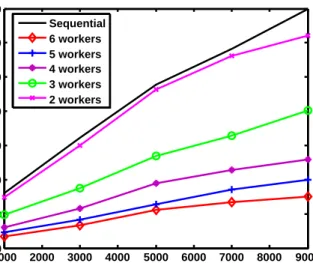
fusion rule with dependent measurement noise. . . 42 3.1 The architecture of Storm. . . 44 3.2 The architecture of C-Storm. . . 46 3.3 C-Storm versus sequential baseline in terms of average total processing time. . 52 3.4 Average total processing times of C-Storm with different number of workers
used for obtaining the marginal probability densities in the fusion bolt. . . 53
used for performing the test in the fusion bolt. . . 54
3.6 ROCs for the detection problem. . . 54
4.1 A typical Deep Neural Network structure [84]. . . 58
4.2 R-Vine copula based multi-modal DNN. . . 58
4.3 First level dependence structure for activity ‘Walking-upstairs’. . . 65
5.1 Parallel distributed detection system. . . 70
5.2 Average expected stopping time as a function of α for centralized sequential scheme. . . 86
5.3 Average expected stopping time as a function ofβ for centralized sequential scheme. . . 86
5.4 Truncation windowW0as a function ofα˜andβ˜, whereα˜= ˜β. . . 88
6.1 Two-step cluster-based collaborative distributed estimation system, where the orange dash lines represent the inter-cluster communication links and the black dash lines denote the intra-cluster communication links. . . 94
6.2 Average clustering accuracy as a function of thresholddth. . . 110
6.3 Average clustering accuracy as a function of number of observationsN with dth= 0.83. . . 110
6.4 Average MSE as a function of SNR without sensor selection. . . 111
6.5 Average MSE as a function of the number of observations N without sensor selection. . . 111
6.6 Average MSE as a function of SNR with cluster-based sensor selection and mk = 3. . . 112
6.7 Average MSE as a function of the number of observationsN with cluster-based sensor selection andmk = 3. . . 113
lection. . . 114 6.9 Average MSE as a function of the number of observations N for different
schemes without sensor selection. . . 114 6.10 Average MSE as a function of SNR for the cluster-based sensor selection
scheme and the global sensor selection scheme. . . 115 6.11 Average MSE as a function of the number of observations N for the
cluster-based sensor selection scheme and the global sensor selection scheme. . . 116
C
HAPTER
1
I
NTRODUCTION
The problem of inference by fusing data from multiple modalities has a wide variety of ap-plications, such as activity monitoring, autonomous robotics and military/security surveil-lance. Typically, a large number of spatially distributed sensors are deployed in a network and these sensors operate collaboratively to solve an inference problem, such as detection, estimation and classification. Fusing observations of multiple sensors can improve decision making and provide global information of a certain phenomenon. However, sensors used for observing the same phenomenon are usually of different modalities, namely, they are incom-mensurate/heterogeneous. Sensors are said to be heterogeneous if their respective observation models cannot be described by the same statistical distribution. Moreover, sensor observations are often dependent due to a variety of reasons such as sensing of the same phenomenon. The nature of this dependence can be quite complex and nonlinear, especially in cases where the signal may propagate through a non-homogeneous medium. Inference in such multi-sensor systems is the major topic of this thesis.
In networks with limited communication resources, local observations are usually com-pressed at the sensors according to certain local rules, and only the comcom-pressed information is transmitted to the FC. In such distributed networks, the challenge is to achieve high
perfor-mance in terms of accuracy efficiency and time efficiency while satisfying energy and band-width constraints. The existence of nonlinear cross-modal dependence and heterogeneity of sensors in the network make the design of local inference rules and the fusion rule at the FC highly complex. In terms of accuracy, we study the design of local and fusion rules in this thesis, where we take the underlying spatial dependence into consideration to improve infer-ence performance. In terms of time efficiency, we consider a distributed sequential network, and design sequential tests at the local sensors and a copula based sequential test at the FC. A parallel platform for fusing heterogenous streaming data is also investigated to accelerate infer-ence response. Moreover, in a fully distributed network with no FC, intra-cluster collaboration and inter-cluster collaboration are studied to exploit the underlying dependence among sensors so that inference performance is improved to the largest extent under limited communication budget.
1.1
Background
Copula theory, which forms the basis of a lot of work in this thesis, is presented in this section. Copulas provide a flexible and powerful approach for modeling underlying dependence among continuous random variables. A multivariate copula, specified independently from marginals, is a multivariate distribution with uniform marginal distributions. The unique correspondence between a multivariate copula and any multivariate distribution is stated in Sklar’s theorem [75] which is a fundamental theorem of copula theory. Standard well defined multivariate copulas may lack the ability to model high dimensional nonlinear dependencies due to factors such as limited number of parameters to characterize the dependence. Based on this, regular vine copula based methodology has been developed for more flexible modeling of dependencies in larger dimensions. In the following, we first give the theoretical background of copula theory and present some well defined multivariate copulas, and then introduce the regular vine copula.
1.1.1
Copula Theory
Theorem 1.1(Sklar’s Theorem). The joint distribution functionF of random variablesx1, . . . , xd
with continuous marginal distribution functionsF1, . . . , Fdcan be cast as
F(x1, x2, . . . , xd) =C(F1(x1), F2(x2), . . . , Fd(xd)|φ), (1.1)
whereCis a uniqued-dimensional copula with dependence parameterφ. Conversely, given a copulaCand univariate Cumulative Distribution Functions (CDFs)F1, . . . , Fd,F in Equation
(1.1)is a valid multivariate CDF with marginalsF1, . . . , Fd. Note thatφis used to characterize
the amount of dependence among thed random variables. In general, φmay be a scalar, a vector or a matrix.
For absolutely continuous distributions F and F1, . . . , Fd, the joint Probability Density
Function (PDF) of random variablesx1, . . . , xdcan be obtained by differentiating both sides of
Equation (1.1): f(x1, . . . , xd) = Yd m=1 fm(xm) c(F1(x1), . . . , Fd(xd)|φ), (1.2)
wheref1, . . . , fd are the marginal densities and cis referred to as the density of multivariate
copulaCthat is given by
c(u|φ) = ∂ d(C(u 1, . . . , ud|φ)) ∂u1, . . . , ∂ud , (1.3) whereum =Fm(xm)andu= [u1, . . . , ud].
Thus, given specified univariate marginal distributionsF1, . . . , Fdand the copula modelC,
the joint distribution functionF can be constructed by
where um = Fm(xm) and Fm−1(um) are the inverse distribution functions of the marginals,
m= 1,2, . . . , d.
Note thatC(·|φ)is a valid CDF andc(·|φ)is a valid PDF for uniformly distributed random variablesum, m = 1,2, . . . , d. Since different copula functions may model different types of
dependence, selection of copula functions to characterize joint statistics of random variables is a key problem. Various families of multivariate copula functions are described in [75]. A brief summary of some popularly used copula functions is provided next.
1.1.2
Summary of Some Multivariate Copula Functions
Elliptical copulas
The Gaussian and the Student-t copula functions belong to the family of elliptical copulas. They are derived from multivariate Gaussian and Student-t distributions, respectively. They both specify dependence using the correlation matrix and are given as follows.
The multivariate Gaussian copula, derived from ad-dimensional multivariate Gaussian dis-tribution, is defined as
CG(u|Σ) = ΦΣ(Φ−1(u1), . . . ,Φ−1(ud)), (1.5)
whereΣis the correlation matrix,Φis the univariate normal CDF andΦΣdenotes the
multi-variate normal CDF.
Similarly, the Student-tcopula is derived from ad-dimensional multivariate Student-t dis-tribution, which is given by
Ct(u|Σ, ν) = tν,Σ(tν−1(u1), . . . , t−ν1(ud)), (1.6)
de-grees of freedom ν (ν ≥ 3), and tν is the univariate Student-t distribution with degrees of
freedomν. It is common to set ν = 3to incorporate heavy tail dependence. As ν → ∞, the Student-tcopula approaches the Gaussian copula function.
Archimedean copulas
Archimedean copulas are defined as follows,
C(u|φ) = Ψ−1 d X m=1 Ψ(um) ! , (1.7)
where we refer toΨ(·)as the generator function andφas the parameter of the copula. Some Archimedean copula functions are indicated in Table 1.1 [41].
Table 1.1: Archimedean copula functions.
Copula Generator FunctionΨ Copulas in the Parametric Form Clayton φ1 u−φ−1 Pd m=1u −φ m −1 −φ1 , φ∈[−1,∞)\{0}
Frank −log expexp{−{−φuφ}−}−11 −1
φlog 1 + Qd m=1[exp{−φum}−1] exp{−φ}−1 , φ∈R\{0} Gumbel −lnuφ exp −Pd m=1(−lnum)φ 1φ , φ∈[1,∞) Independent −lnu Qd m=1um
1.1.3
Copulas and Measures of Dependence
An attractive feature of copulas is that nonparametric rank-based measures of dependence, such as Kendall’sτ, can be expressed as expectations over the copula distribution. For independent pairs of random variables(X1, Y1)and(X2, Y2)having the same distribution as(X, Y),
con-cordance is defined as the condition that(X1−X2)(Y1−Y2)≥0and discordance is defined as
the probabilities of concordance and discordance:
τ ,P[(X1−X2)(Y1−Y2)≥0]−P[(X1 −X2)(Y1−Y2)<0].
Nelsen has proved the relationship in Equation (1.8) for a copula,C(·|φ), and random variables
X ∼fX(x), Y ∼fY(y)[75], i.e.,
τ(φ) = 4
Z Z
[0,1]2
C(FX(x), FY(y)|φ)dC(FX(x), FY(y)|φ)−1. (1.8)
This relationship allows τ to be expressed in terms of the dependence parameter of the copula, C (Σfor the elliptical copulas andφfor the Archimedean copulas in Table 1.1). For the case of elliptical copulas, parametrized by the matrixΣ = [ρij],
ρij = sin
πτij
2
, (1.9)
whereτij is the Kendall’s τ evaluated for the pair (Ui, Uj) = (FXi(·), FXj(·)). The sample
estimate of Kendall’sτ, forN observations, can be calculated as the ratio of the difference in the number of concordant pairs,ccor, and discordant pairs,dcor, to the total number of pairs of
observations, i.e., ˆ τ = ccor−dcor ccor+dcor = ccor−N dcor 2 . (1.10)
Typically, φis unknown a priori and needs to be estimated, e.g., using Maximum Like-lihood Estimation (MLE) [41]. On the other hand, Equation (1.8) and Equation (1.10) imply that Kendall’sτ can be used for calculating computationally efficient estimates ofφ.
1.1.4
Regular Vine Copula
Regular vine (R-Vine) copulas, introduced by Bedford and Cooke in [11, 12], are extremely flexible in modeling high dimensional multivariate dependence, where a set of bivariate
cop-ulas are used to construct the multivariate copula. A regular vine copula is a tree-structured graphical model that consists of a regular vine and a set of bivariate copulas. We first present the definition of the regular vine in the following. A regular vine is defined as follows.
Definition 1.1(R-Vine). V = (T1, . . . , Td−1)is a regular vine ond elements if the following
conditions are satisfied.
1. T1is a tree with nodesN1 ={1, . . . , d}and a set ofd−1edges denoted asE1.
2. Fori= 2, . . . , d−1,Tiis a tree with nodesNi =Ei−1and edge setEi.
3. Fori = 2, . . . , d−1and{a, b} ∈Ei witha ={a1, a2}andb = {b1, b2}, |(a∩b)|= 1
(proximity condition) holds, where| · |denotes the cardinality of a set.
Ad-dimensional vine consists ofd(d−1)/2edges in total. The proximity condition implies that two edges in treeTi are connected in treeTi+1 if the two edges share a common node in
treeTi.
R-Vine copula is obtained by specifying bivariate copulas, the so-called pair-copula, on each of the edges. Before introducing R-Vine copula, some sets associated with its edges need to be defined. The complete union Ue of an edge e = {a, b} ∈ Ei, a, b ∈ Ni is defined as
Ue = {m ∈ N1| ∃ej ∈ Ej, j = 1,2, . . . , i − 1,such thatm ∈ e1 ∈ . . . ei−1 ∈ e}. The
conditioning set of the edgee = {a, b}isDe = Ua∩Ub and the conditioned sets of the edge
e={a, b}areCe,a=Ua\DeandCe,b=Ub\De. A regular vine copula is defined as follows.
Definition 1.2(R-Vine Copula). (F,V,B)is called a R-Vine copula if 1. F= [F1, F2, . . . , Fd]T ∈[0,1]dis a vector with uniform marginals.
2. V is ad-dimensional regular vine.
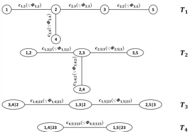
𝑻𝑻𝟏𝟏 𝑻𝑻𝟐𝟐 𝑻𝑻𝟑𝟑 1 2 3 4 𝒄𝒄𝟏𝟏,𝟐𝟐(�;𝜱𝜱𝟏𝟏,𝟐𝟐) 𝒄𝒄𝟐𝟐,𝟒𝟒 ( � ; 𝜱𝜱𝟐𝟐, 𝟒𝟒 ) 𝒄𝒄𝟐𝟐,𝟑𝟑(�;𝜱𝜱𝟐𝟐,𝟑𝟑) 5 𝒄𝒄𝟑𝟑,𝟓𝟓(�;𝜱𝜱𝟑𝟑,𝟓𝟓) 𝒄𝒄𝟑𝟑,𝟒𝟒 | 𝟐𝟐 ( � ; 𝜱𝜱𝟑𝟑, 𝟒𝟒 | 𝟐𝟐 ) 1,2 𝒄𝒄𝟏𝟏,𝟑𝟑|𝟐𝟐(�;𝜱𝜱𝟏𝟏,𝟑𝟑|𝟐𝟐) 2,3 𝒄𝒄𝟐𝟐,𝟓𝟓|𝟑𝟑(�;𝜱𝜱𝟐𝟐,𝟓𝟓|𝟑𝟑) 3,5 2,4 1,3|2 3,4|2 𝒄𝒄𝟏𝟏,𝟒𝟒|𝟐𝟐𝟑𝟑(�;𝜱𝜱𝟏𝟏,𝟒𝟒|𝟐𝟐𝟑𝟑) 𝒄𝒄𝟏𝟏,𝟓𝟓|𝟐𝟐𝟑𝟑(�;𝜱𝜱𝟏𝟏,𝟓𝟓|𝟐𝟐𝟑𝟑) 2,5|3 1,4|23 𝒄𝒄𝟒𝟒,𝟓𝟓|𝟏𝟏𝟐𝟐𝟑𝟑(�;𝜱𝜱𝟒𝟒,𝟓𝟓|𝟏𝟏𝟐𝟐𝟑𝟑) 1,5|23 𝑻𝑻𝟒𝟒
Fig. 1.1: An example R-Vine for five variables. The joint density of a random vectorx= [x1, x2, . . . , xd]T is given by
f1,...,d(x) = d Y m=1 fm(xm) d−1 Y i=1 Y e∈Ei
×cCe,a,Ce,b|De(FCe,a|De(xCe,a|xDe), FCe,b|De(xCe,b|xDe)),
(1.11)
wheree ={a, b},xDe ={xj|j ∈De}, fm is the marginal PDF of variablexm,m = 1, . . . , d.
The conditional distributionFCe,a|De(xCe,a|xDe)can be obtained recursively tree by tree by the
following equation [51].
FCe,a|De(xCe,a|xDe) =
∂CCa,a1,Ca,a2|Da FCa,a1|Da(xCa,a1|xDa), FCa,a2|Da(xCa,a2|xDa)
∂FCa,a2|Da(xCa,a2|xDa)
, (1.12)
wheree ={a, b} ∈ Ei, a ={a1, a2}andb ={b1, b2}are the edges that connect Ce,aandCe,b
given the conditioning variablesDe. Similarly, we can obtainFCe,b|De(xCe,b|xDe).
As an example, a 5-dimensional R-Vine copula is shown in Fig. 1.1. The R-Vine has four trees Ti and the tree Ti has nodes Ni = 6−i and edges Ei = 5−i, where i = 1,2,3,4.
Each edge is associated with a bivariate copula density cand its corresponding parametersφ
used to model dependence between two variables. Moreover, at each edge e = {a, b} ∈ Ei,
De appears on the right. In the first tree T1, the dependences of the four pairs of variables (1,2),(2,3),(2,4),(3,5) are modeled using four bivariate copulas, c1,2(·;φ1,2), c2,3(·;φ2,3), c2,4(·;φ2,4)andc3,5(·;φ3,5). In the second treeT2, three conditional dependencies are modeled.
The pair (1,3|2) using bivariate copula density c1,3|2(·;φ1,3|2) characterizes the dependence
between the first and third variables given the second variable. Also, the pair (3,4|2) using bivariate copula density c3,4|2(·;φ3,4|2) characterizes the dependence between the third and
fourth variables given the second variable. Similarly, we can obtain the bivariate copula density for the pair(2,5|3). In the third treeT3, the dependence of the first and fourth variables given
the second and third variables is modeled using bivariate copula densityc1,4|23(·;φ1,4|23). Also,
we can obtain the bivariate copula density for the pair (1,5|23). In the fourth tree T4, the
bivariate copula density c4,5|123(·;φ4,5|123) captures the dependence between the fourth and
fifth variables given the first, second and third variables.
For the 5-dimensional case, using Equation (1.11), the joint PDF ofz = [z1, z2, z3, z4, z5]
can be expressed as f(z1, z2, z3, z4, z5) = " 5 Y l=1 f(zl) # ·c1,2 F(z1), F(z2);φ1,2 ·c2,3 F(z2), F(z3);φ2,3 ·c2,4 F(z2), F(z4);φ2,4 ·c3,5 F(z2), F(z3)·;φ3,5 ·c1,3|2 F(z1|z2), F(z3|z2);φ1,3|2 ·c3,4|2 F(z3|z2), F(z4|z2);φ3,4|2 ·c2,5|3 F(z2|z3), F(z5|z3);φ2,5|3 ·c1,4|23 F(z1|z2z3), F(z4|z2z3);φ1,4|23 ·c1,5|23 F(z1|z2z3), F(z5|z2z3);φ1,5|23 ·c4,5|123 F(z4|z1z2z3), F(z5|z1z2z3);φ4,5|123 . (1.13)
1.1.5
Array Representation of Regular Vine
Generally, it is quite expensive to store the nested set of trees and also not convenient to de-scribe inference algorithms. In [72], a lower triangular array was proposed to store a R-Vine.
Definition 1.3 (R-Vine Array). A lower triangular array M = (mi,j)i,j=1,2,...,d is called a
R-Vine array if fori= 1, . . . , d−1and for allk =i+ 1, . . . , d−1, there is ajini+ 1, . . . , d−1
with(mk,i,{mk+1,i, . . . , md,i}) ∈ BM(j)or ∈ B˜M(j), whereBM(j) := {(mj,j, D)|k = j +
1, . . . , d} with D = {mk,j, . . . , md,j} and B˜M(j) := {(mk,j,D˜)|k = j + 1, . . . , d} with
˜
D={mj,j} ∪ {mk+1,j, . . . , md,j}.
For the R-Vine copula example in Fig. 1.1, the R-Vine matrixM∗ is given as
5 4 4 1 1 1 2 3 3 3 3 2 2 2 2 ,
where the first column represents the dependence of four pairs of variables,(5,4|123),(5,1|23),
(5,2|3)and(5,3). Going through all columns, we can see that the matrixM∗ codes all infor-mation needed to represent the R-vine copula in Fig. 1.1.
An R-Vine array has the following two properties:
• {mi,i, . . . , md,i} ⊂ {mj,j, . . . , md,i}for1≤j < i≤d,
• mi,i ∈ {m/ i+1,i+1, . . . , md,i+1}fori= 1, . . . , d−1,
where the first property states that every column in the left contains all the entries that a col-umn in the right contains, and the second property guarantees that there is a new entry on the diagonal in every column.
Given an R-Vine arrayM = (mi,j)i,j=1,...,d, the R-Vine copula based modeling of the joint PDF [27] is f1,...,d = d Y j=1 fj 1 Y k=d−1 k+1 Y i=d cmk,k,mi,k|mi+1,k,...,md,k Fmk,k|mi+1,k,...,md,k, Fmi,k|mi+1,k,...,md,k . (1.14)
For notational simplicity, we have removed the arguments of all the functions in Equation (1.14).
1.2
Literature Review
Multimodal signal processing enables fusion of information from several sources in order to form a unified picture and produce a global decision/estimation. There are mainly three fusion strategies: data-level fusion, feature-level fusion and decision-level fusion. Signal process-ing for inference problems with distributed sensors has been studied extensively. Centralized
inference (also known as data-level fusion), where raw observations are available at the pro-cessing unit or FC, have been well studied in standard textbooks [13, 59, 101]. Distributed
inference, on the other hand, relies on the topology of a network that can either transmit a com-pressed/processed version of the raw data to the FC (can be feature-level fusion or decision-level fusion) or arrive at a consensus solution by locally sharing compressed/processed infor-mation (e.g., see [55, 56, 67, 78, 105, 117] and references cited therein).
This section reviews some recent progress that has been made in the field of multimodal signal processing, and focuses on developments where data dependence plays a significant role in the design of fusion rules for inference problems. The aim of this discussion is to motivate our current research.
1.2.1
Linear Dependence: Covariance Matrix
Covariance matrix, or equivalently correlation matrix, models linear dependence among jointly normal random variables or variables that possess a finite second moment. In networks with multiple sensors/sources, it is used extensively to model dependency information across the sensors/sources, especially where it is reasonable to assume linearity of the medium of sig-nal propagation. In MIMO systems, the dependence among multiple antennas/channels was modeled in [52, 63, 71]. In [4], linear dependence among multiple datasets was characterized for joint blind source separation. Canonical correlation analysis (CCA) has also been used to perform feature-level information fusion for recognition problems [29, 35, 39].
Optimal schemes for distributed detection and estimation with dependent observations have also been a topic of significant interest. In the case of distributed detection, it has been shown in [105] that the optimal sensor decision rule is the likelihood-ratio-based binary quantizer, and the optimal fusion statistic at the FC is a weighted sum of sensor decisions under the as-sumption of conditional independence. These sensor decision rules and fusion statistic are no longer optimal when correlation is taken into account. Examples of the consequent loss in performance were presented in [1]. Moreover, it has been shown in [102] that the distributed detection problem with dependent observations is NP-complete and cannot be solved using a polynomial time algorithm. Therefore, the design of optimal local decision rules may not be possible due to computational intractability resulting from the dependence among sensor observations. One way to get past the computational intractability is to assume some prior in-formation about the joint statistics, e.g., in [28, 57], fusion rules for correlated binary decisions were studied by considering known correlation coefficients and known correlated sensing noise PDFs, respectively. Another way is to constrain local detectors to be binary quantizers and de-sign optimal fusion rules at the FC, e.g., in [18, 109], optimal fusion rules were proposed with correlated Gaussian noise. Also, in [58], noisy correlated sensing channels were studied for multi-bit decision based distributed detection and a likelihood ratio test was used to generate
the global decision at the FC.
The distributed estimation problem by modeling dependent observations has been studied in [32, 61, 66]. In [61], a distributed estimation scheme was studied with multivariate Gaussian correlated sensor observations and the covariance was assumed to be known at the FC. In [32], the estimation of a random scalar parameter in a power constrained wireless sensor network was studied with generally correlated sensor observations that can accommodate nonlinear measurement models and spatially correlated observation noise. The goal was to design opti-mal power allocation strategy. In [66], the problem of sensor selection for parameter estimation was considered with spatially correlated Gaussian measurement noise and the aim was to seek optimal sensor activations by formulating an optimization problem which minimizes estimation error subject to energy constraints. Besides these formulations, designing estimation schemes in the presence of dependent data often gives rise to intractable problem formulations. In such situations, applying well-known strategies derived from conditional independence assumption may turn out to be fairly suboptimal. One way to address this issue is to allow inter-sensor communication/collaboration instead of modeling this dependence [16, 20, 31, 55, 56, 67, 87]. In [31, 56, 67], collaborative distributed estimation problems with a fusion center were con-sidered, where collaboration was restricted to be a linear operation. Collaborative distributed estimation problems without a FC were studied in [16, 20, 55, 87], where different distributed collaboration strategies were proposed, such as diffusion-based, consensus-based and gossip-based algorithms.
1.2.2
Nonlinear Dependence: Nonparametric Approach
Multimodal signal processing using nonparametric approaches has attracted significant atten-tion in applicaatten-tions where it is infeasible to model the complex nonlinear dependencies that may exist among sensor observations/features. These methods, in essence, estimate or learn the joint distribution across sensor observations/features directly from the data.
Information theoretic approaches make it possible to characterize arbitrary nonlinear de-pendence compared to methods using covariance matrix. In [15], mutual information and joint entropy based methodologies were proposed to model the underlying dependence between au-dio and video data. In [14,40,85], mutual information based methods were proposed for image fusion. Graphical models such as Bayesian networks generalize hidden Markov models and have also been successfully used for multimodal fusion (see e.g. [23, 53, 81, 96]).
Machine learning and deep learning techniques have had breakthroughs in a wide range of multimodal applications: from audio-visual speech recognition to image captioning [7, 8, 38, 86]. The advantage of machine learning and deep learning based methodologies is that they can extract significant amount of information from sensor data with no need of modeling the joint distribution of the data. There are plenty of networks including shallow networks, such as Support Vector Machines (SVMs), Random Forests and Decision Trees, and deep networks, such as deep forward neural networks and convolutional neural networks. Compared to the shallow networks, the deep networks can learn high-level features directly from raw data (or lightly processed data) and provide joint representations for multimodal data.
1.2.3
Nonlinear Dependence: Copula-based Approach
Recall from Section 1.1 that copulas are parametric functions that can model nonlinear depen-dence among multiple random variables. The copula based dependepen-dence modeling approach is attractive and powerful because it can characterize potentially any nonlinear spatial depen-dence among sensor observations and allow different marginal distributions. Moreover, while nonparametric approaches have shown their superiority in characterizing the joint distribution among multimodal data, they also suffer from issues, such as scalability problems stemming from the curse of dimensionality (information theoretic/graphical model based approaches) and the availability of enough training data (deep learning based approaches). Recently, con-siderable progress has been made in the study of copulas and their applications in statistics.
The usage of copulas is widespread in the fields of econometrics and finance [19] and they are beginning to be used in the signal and image processing context [24, 42, 48, 70, 93].
Multivariate copula based approaches have shown their superiority in improving the per-formance of inference problems [43, 45, 50, 94, 95]. In [50], a general framework of copula based detection has been investigated. The performance loss due to copula misspecification was quantified. The efficacy of the proposed copula based detection scheme was demonstrated using a NIST multibiometric dataset. In [95], the problem of distributed detection has been studied, where a copula based optimum fusion rule was derived for a Neyman-Pearson detector. In [45], the utility of non-stationary dependence modeling with copulas has been considered for detecting the presence of a phenomenon being observed jointly by heterogeneous sensors. In [94], a copula-based estimation scheme has been proposed for the localization of a radiation source, and the overall estimation performance was shown to be improved by taking the under-lying dependence among sensor observations into account. In [43], the fusion of social media and sensor data has been addressed using the copula-based dependence modeling approach.
However, the class of known multivariate copulas required for the fusion of observations from more than two sensors is limited. Gaussian copulas perform poorly on data with heavy tails. Student-t copulas allow for symmetric tail dependence, but they have only a single pa-rameter to capture tail dependence among all the variables. While standard Archimedean mul-tivariate copulas can characterize asymmetric tail dependence, they are quite limited as they are characterized by only a single parameter. This shows that there is a growing need for more flexible copulas especially for modeling high-dimensional dependence structures. Vine copu-las, tree-structured graphical models, are more flexible and powerful compared to multivariate copulas, where a set of bivariate copulas are used to construct the multivariate copula [2,11,12].
1.3
Main Contributions and Organization
The main contributions of the research results presented in this dissertation to the signal pro-cessing and information fusion literature, are as follows:
In Chapter 2, we propose a regular vine copula based methodology for the fusion of sta-tistically dependent decisions. Regular vine copula can express a multivariate copula by using a cascade of bivariate copulas, the so-called pair copulas. Assuming that local detectors are single threshold binary quantizers and taking complex dependence among sensor decisions into account, we design an optimal fusion rule using a regular vine copula under the Neyman-Pearson framework. In order to reduce the computational complexity resulting from the com-plex dependence, we propose an efficient and computationally light regular vine copula based optimal fusion algorithm. Numerical experiments are conducted to demonstrate the effective-ness of our approach.
Nowadays, we are inundated by a large amount of streaming data that are generated con-tinuously with high arrival rates from sources such as sensors and social media. The methods applied for processing data streams should be fast enough to keep up with the high arrival rate of incoming data, and at the same time provide solutions for inference problems (detection, classification, or estimation) with high accuracies. In Chapter 3, we design a novel parallel platform, C-Storm (Copula-based Storm), for the computationally complex problem of fusion of heterogeneous data streams for inference. C-Storm is designed by marrying copula-based dependence modeling for highly accurate inference and a highly-regarded parallel computing platform Storm for fast stream data processing. C-Storm has the following desirable features: 1) C-Storm offers fast inference responses. 2) C-Storm provides high inference accuracies. 3) C-Storm is a general-purpose inference platform that can support data fusion applications. 4) C-Storm is easy to use and its users do not need to have deep knowledge of Storm or copula theory.
the fusion of multiple deep neural network classifiers. We take the cross-modal dependence into account by employing regular vine copulas to characterize complex dependence among multiple modalities. More specifically, multiple deep neural networks are used to extract high-level features from multiple sensing modalities, with each deep neural network processing the data collected from a single sensor. The extracted high-level features are then combined using a regular vine copula model. Numerical experiments are conducted to demonstrate the effectiveness of our approach.
In Chapter 5, we consider the problem of distributed sequential detection using wireless sensor networks in the presence of imperfect communication channels between the sensors and the fusion center. Sensor observations are assumed to be spatially dependent. Moreover, the channel noise can be dependent and non-Gaussian. We propose a copula based distributed sequential detection scheme that takes the spatial dependence into account. More specifically, each local sensor runs a memory-less truncated sequential test repeatedly and sends its binary decisions to the fusion center synchronously. The fusion center fuses the received messages using a copula-based sequential test. To this end, we first propose a centralized copula based se-quential test and show its asymptotic optimality and time efficiency. We then show the asymp-totic optimality and time efficiency of the proposed distributed scheme. We also show that by suitably designing the local thresholds and the truncation window, the local probabilities of false alarm and miss detection of the proposed memory-less truncated local sequential tests sat-isfy the pre-specified error probabilities. Numerical experiments are conducted to demonstrate the effectiveness of our approach.
In Chapter 6, we consider the problem of collaborative distributed estimation in a large scale sensor network with statistically dependent sensor observations. In the collaborative setup, the aim is to maximize the overall estimation performance by modeling the underlying statistical dependence and efficiently utilizing the deployed sensors. To achieve greater sen-sor transmission and estimation efficiency, we propose a two-step cluster-based collaborative
distributed estimation scheme, where in the first step, sensors form dependence driven clusters such that sensors in the same cluster are dependent, while sensors from different clusters are independent, and perform copula-based maximum a posteriori probability (MAP) estimation via intra-cluster collaboration. In the second step, the estimates generated in the first step are shared via inter-cluster collaboration to reach an average consensus. A merge basedK-medoid dependence driven clustering algorithm is proposed. Moreover, we further propose a cluster-based sensor selection scheme using mutual information prior to the estimation. The aim is to select sensors with maximum relevance and minimum redundancy regarding the parameter of interest under certain pre-specified energy constraint. Also, the proposed cluster-based sensor selection scheme is shown to be equivalent to the global/non-cluster based selection scheme with high probability, which at the same time is computationally more efficient. Numerical simulations are conducted to demonstrate the effectiveness of our approach.
Finally, in Chapter 7, we summarize the findings and results of this dissertation. Several directions and ideas for future research are also presented.
1.4
Bibliographic Note
Part of the work presented in this dissertation has appeared in the following publications: 1. Shan Zhang, Jielong Xu, Sora Choi, Jian Tang, Pramod K. Varshney, and Zhenhua Chen,
“A Parallel Platform for Fusion of Heterogeneous Stream Data," inProc. 21th Interna-tional Conference on Information Fusion, 2018.
2. Shan Zhang, Baocheng Geng, Pramod K. Varshney, and Muralidhar Rangaswamy, “Fu-sion of Deep Neural Networks for Activity Recognition: A Regular Vine Copula Based Approach," inProc. 22th International Conference on Information Fusion, 2019. 3. Shan Zhang, Prashant Khanduri, and Pramod K. Varshney, “Distributed Sequential
Conference on Signals Systems and Computer, 2019.
4. Shan Zhang, Lakshmi N. Theagarajan, Sora Choi, and Pramod K. Varshney, “Fusion of Correlated Decisions Using Regular Vine Copulas," IEEE Transactions on Signal Processing, vol 67, no. 8, pp. 2066-2079, 2019.
5. Shan Zhang, Prashant Khanduri, and Pramod K. Varshney, “Distributed Sequential De-tection: Dependent Observations and Imperfect Communication,"IEEE Transactions on Signal Processing, accepted, 2019.
6. Shan Zhang, Pranay Sharma, and Pramod K. Varshney, “Distributed Estimation in Large Scale Wireless Sensor Networks via A Two-Step Cluster-based Approach," to be sub-mitted, 2019.
C
HAPTER
2
D
ISTRIBUTED
D
ETECTION
B
ASED ON
R
EGULAR
V
INE
C
OPULAS
2.1
Motivation
Fusion of data from heterogeneous sensors/sources has been shown to improve the performance of inference tasks. In many practical cases, these sensor observations are dependent due to a variety of reasons such as sensing of the same phenomenon and dependent transmission channels. Ignoring this dependence may degrade inference performance.
In this chapter, we consider the problem of distributed detection with dependent sensor ob-servations under the Neyman-Pearson framework. We assume that local detectors are single threshold binary quantizers, and the aim is to derive an optimal fusion rule at the FC by taking the dependent decisions into consideration. We propose a novel and powerful fusion method-ology for the fusion of dependent decisions, R-Vine copula based fusion, for more flexible modeling of complex dependency especially for larger number of sensors. In order to reduce the computational complexity resulting from the complex dependence, we further propose an efficient and computationally light regular vine copula based optimal fusion algorithm.
2.2
Problem Formulation
Consider a distributed detection problem, where a random phenomenon is monitored by L
sensors. A binary hypothesis testing problem is studied, where H1 denotes the presence of
the random phenomenon and H0 denotes the absence of the phenomenon. The sensors make
a set of observations at time instant n, zn = [z1n, z2n, . . . , zLn], n = 1,2, . . . , N. We assume
that the sensor observations are dependent across sensors. Moreover, we further assume that the sensor observations are continuous random variables that are conditionally independent and identically distributed (i.i.d.) over time. Letf(zln|H1)andf(zln|H0)be the PDFs of the
observation at thelth sensor andnth time instant underH1andH0hypotheses, respectively. No
knowledge about the joint distribution of the sensor observations is availablea priori. Instead of transmitting noisy raw observations, local binary sensor decisionsulnare sent to the FC by
using a binary quantizer which is defined as
uln= 0 −∞< zln < τl 1 τl ≤zln<+∞ , (2.1)
where τl is the quantizer threshold at the lth sensor. At the FC, local binary decisions are
combined to obtain a global decision.
Under the Neyman-Pearson criterion, the design problem for the parallel distributed detec-tion system consists of deriving individual sensor thresholdsτl to form sensor decisions and
the optimal fusion rule that fuses local sensor decisions to obtain the global decision. The sen-sor thresholdsτl, l = 1,2, . . . , Lare obtained by maximizing the local probability of detection
subject to a constraint on the local probability of false alarm. Note that these sensor thresh-olds are not necessarily optimal in the global sense. The design of the optimal fusion rule for multiple sensors is discussed next.
Since sensor decisions are independent over time, the optimal test statistic [104] is given as Λ(u) = QN n=1P(u1n, u2n, . . . , uLn|H1) QN n=1P(u1n, u2n, . . . , uLn|H0) , (2.2)
whereP(u1n, u2n, . . . , uLn|Hk)is the joint probability mass function (PMF) of the sensor
deci-sions at thenth time instant underkth hypothesis,k = 0,1. We defineS ={u1nu2n. . . uLn|uln∈
{0,1}, l = 1,2, . . . , L}as the set of all permutations that specify L-sensor decisions at time instant n. There are a total of 2L permutations for L sensors. For a three-sensor problem,
S={{000},{001},{010},{011},{100},{101},{110},{111}}. Let
P(u1n, u2n, . . . , uLn|H1) = Ps, and
P(u1n, u2n, . . . , uLn|H0) = Qs,
(2.3)
where s ∈ S. Ps and Qs, s ∈ S are required while computing the test statistic at the FC.
For a three-sensor problem, the set of probabilitiesP000, P001, P010, . . .,P111 andQ000, Q001, Q010, . . ., Q111 that characterize the joint PMFs of sensor decisions u1n, u2n and u3n under
hypothesesH1 andH0, respectively, are needed. By integrating the joint PDFs of the sensor
observations under both hypotheses, these probabilities can be obtained with the quantizer thresholdτl,l = 1,2,3. For example,
P000 = Z τ1 z1=−∞ Z τ2 z2=−∞ Z τ3 z3=−∞ f(z1, z2, z3|H1)dz1dz2dz3, P010 = Z τ1 z1=−∞ Z z2=+∞ τ2 Z τ3 z3=−∞ f(z1, z2, z3|H1)dz1dz2dz3, (2.4)
where for the simplification of notation, we omit the time indexnin the example.
However, due to existing complex and nonlinear dependence, the joint PDFs of sensor observations under both hypotheses are not known. Before determining the joint PMFs of sensor decisions, we first need to obtain the joint PDFs of sensor observations given only the knowledge of marginal PDFs of the sensor observations and the marginal PMFs of sensor
decisions. Typically in many applications, we do not have any prior information related to the phenomenon of interest. Therefore, we may also need to determine the marginals of sensor observations.
The dependence across sensors can be quite complicated and nonlinear. Simple dependence modeling through methods such as the use of multivariate normal model, is very limited and in-adequate to characterize complex dependence among multiple sensors. Assuming conditional independence among multiple sensors may result in substantial performance degradation. To design the optimal fusion rule, we propose a copula based fusion methodology to characterize the existing dependence and determine the joint PDFs of sensor observations. Due to the lim-itations of the class of standard multivariate copulas and complex dependence that generally exists among multiple sensors, more flexible dependence modeling approaches are needed to obtain the joint PDFs of sensor measurements. R-Vine copula based dependence modeling provides us a solution. It can express a multivariate copula using a cascade of bivariate copulas embedded in a tree structure that is shown to be more flexible and powerful to model the com-plex dependence. Note that learning of the joint distribution requires raw sensor observations. It can be done offline. Here, we assume that the joint statistics of the sensors does not change over time. After measurement collection, raw measurements are sent to the FC. The FC uses these analog measurements to learn the joint statistics of the sensors. After that, only binary decisions are sent to the FC.
Taking the above considerations into account, in the following, we develop a novel and powerful R-Vine copula based fusion methodology for distributed detection. We will propose the optimal test statistic for the parallel distributed detection system and derive its asymptotic statistic when the number of observations is large. Furthermore, at the end, via simulations, we will show its power and flexibility to capture complex dependence and improve detection performance.
2.3
R-Vine Copula Based Fusion of Multiple Statistically
Dependent Decisions
2.3.1
Optimal Test Statistic
The optimal test statistic for Lsensors is characterized in Equation (2.2). The joint PMF of
uln,l= 1,2, . . . , L, at timen,n= 1,2, . . . , N underH1 andH0, respectively, is given as: P(u1n, u2n, . . . , uLn|H1) = Y s∈S PQLl=1xln s , P(u1n, u2n, . . . , uLn|H0) = Y s∈S QQLl=1xln s , (2.5)
whereslindicates thelth element ofs, andxln = uln ifsl = 1, otherwise,xln = 1−uln for
s ∈ S. For example, please see Equation (2.7) and Equation (2.8), which are special cases of Equation (2.5) forL= 3.
Substituting Equation (2.5) in Equation (2.2) and taking log on both sides, the log test statistic is given by logΛ(u) = X {i1n}∈I1 Au1 N X n=1 u1 + X {i1n,i2n}∈I2 Au2 N X n=1 u2+. . .+ (2.6) X {i1n,i2n,...,itn}∈It Aut N X n=1 ut+. . .+ X {i1n,i2n,...,iLn}∈IL AuL N X n=1 uL
whereI ={ln|uln ∈ {0,1}, l = 1,2, . . . , L, n= 1,2, . . . , N}, Iiis a subset of I and the
car-dinality of the setIi isi, namely,|Ii|=i. Moreover,ut ={ui1nui2n. . . uitn},t∈[1,2, . . . , L]
and its weight is given asAut =log Q 0≤k≤tP (−1)t ˜ Ie tk Q 0≤k≤tQ (−1)t ˜ Io tk Q 0≤k≤tQ (−1)t ˜ Ie tk Q 0≤k≤tP (−1)t ˜ Io tk
which is determined by the joint PMFs of sensor decisions, see Appendix A for details. Also, please see Equation (2.9) as an example forL= 3.
The optimal test statistic for the three-sensor case
Considering the three-sensor case, the joint PMF of u1n, u2nandu3nat any time instant, 1 ≤
n≤N, underH1andH0 is given as follows, respectively,
P(u1n, u2n, u3n|H1) = P(1−u1n)(1−u2n)(1−u3n) 000 P (1−u1n)(1−u2n)u3n 001 P (1−u1n)u2n(1−u3n) 010 P(1−u1n)u2nu3n 011 P u1n(1−u2n)(1−u3n) 100 P u1n(1−u2n)u3n 101 Pu1nu2n(1−u3n) 110 P u1nu2nu3n 111 , (2.7) and P(u1n, u2n, u3n|H0) = Q(1−u1n)(1−u2n)(1−u3n) 000 Q (1−u1n)(1−u2n)u3n 001 Q (1−u1n)u2n(1−u3n) 010 Q(1−u1n)u2nu3n 011 Q u1n(1−u2n)(1−u3n) 100 Q u1n(1−u2n)u3n 101 Qu1nu2n(1−u3n) 110 Q u1nu2nu3n 111 . (2.8)
For simplification of notation, we useA1 toA7 to denote the coefficients ofut, t= 1,2,3.
Substituting Equation (2.7) and Equation (2.8) into Equation (2.2) and taking log on both sides, we get logΛ1(u) = A1 N X n=1 u1n+A2 N X n=1 u2n+A3 N X n=1 u3n+A4 N X n=1 u1nu2n+ A5 N X n=1 u1nu3n+A6 N X n=1 u2nu3n+A7 N X n=1 u1nu2nu3n, (2.9)
where A1 =log Q000P100 P000Q100 , A2 =log Q000P010 P000Q010 , A3 =log Q000P001 P000Q001 , A4 =log P000Q100Q010P110 Q000P100P010Q110 , A5 =log P000Q100Q001P101 Q000P100P001Q101 , A6 =log P000Q010Q001P011 Q000P010P001Q011 , A7 =log Q000P100P010P001Q110Q101Q011P111 P000Q100Q010Q001P110P101P011Q111 .
When sensor decisions among L sensors are conditionally independent, only the term
P
{i1n}∈I1
Au1PN
n=1u
1 in Equation (2.6) is left and the optimal fusion rule reduces to the
Chair-Varshney fusion rule statistic (i.e., weighted sum of sensor decisions [17]). For dependent sensor decisions, the optimal fusion rule depends on both the weighted sum of sensor deci-sions and the weighted sum of the cross products of sensor decideci-sions. The cross products of the sensor decisions are due to dependence among multiple sensors. The joint PMFs of sensor decisions, namelyPsandQs,s ∈S, determine the weights of the optimal test statistic, and can
be obtained by solvingLintegrals on the joint PDFs of the corresponding sensor observations (see the example in Equation (2.4)). In the following subsection, we will propose an R-Vine copula based approach to model existing complex dependence and construct the joint PDFs of sensor observations. After obtaining the joint PMFs and given sensor decisions, the optimal fusion rule is given by
logΛ(u)
H1
≷
H0
γ, (2.10)
whereγis the threshold for the test at the FC.
To characterize the fusion performance at the FC using the system probabilities of detection and false alarm, we consider the asymptotic distribution of the optimal fusion rule statistic underH0 andH1.
Theorem 2.1. The optimal fusion test statistic logΛ(u) is asymptotically (when N is large) Gaussian.
The first and second order statistics of logΛ(u) under both hypotheses are given in Ap-pendix B. Let the first and second order statistics of logΛ(u)be denoted by µ0 andσ20 under H0 andµ1 andσ12 underH1. These can be easily derived using the joint PMFs of sensor
deci-sions. The system probability of detection (PD) and system probability of false alarm (PF) are
then given by PD =Q γ−µ1 σ1 , (2.11) PF =Q γ−µ0 σ0 , (2.12)
where Q(·) is the complementary CDF of the Gaussian distribution. Under the Neyman-Pearson framework and by constrainingPF =α,γ can be obtained by
γ =σ0Q−1(PF) +µ0. (2.13)
Note that the local sensors compress their raw measurements into binary decisions (see Equation (2.1)) prior to their transmission to the FC and the corresponding sensor thresholds are assumed to beτl, l = 1,2, . . . , L. Letτ be the vector of sensor thresholds. Constraining
PF =α,PD can be written as PD(τ) =Q σ0Q−1(PF) +µ0(τ)−µ1(τ) σ1(τ) , (2.14)
whereτ is chosen to maximizePD at a particular value ofPF.
It should be noted that the computational complexity for obtaining the joint PMFs is very high since we need to perform multi-dimensional integration at each time instant. In what follows, we first propose the R-Vine copula based methodology to characterize the joint PDFs of sensor observations and then develop an efficient optimal fusion algorithm based on the R-Vine copula model.
2.3.2
R-Vine Copula Based Dependence Modeling
According to Sklar’s theorem (Section 1.1.1), the joint PDF of sensor observations can be separated into its marginals and the dependence structure that is fully characterized by the copula density (see Equation (1.2)). As indicated earlier, the R-Vine copula model (Section 1.1.4) is more flexible to decompose the joint PDF into its marginals and a cascade of bivariate copula densities. In the following, we will use the R-Vine copula to model the dependence structure and obtain the joint PDF of sensor observations.
In our parallel distributed detection sensor network,L sensors make a set of observations
zn = [z1n, . . . , zLn] at time instant n. Recall that we assume the sensor observations to be
conditionally i.i.d. over time. Therefore, it is sufficient to consider the joint PDF of zn. For
notational convenience, we omit the index nin this subsection and letz = [z1, . . . , zL]be the
L-dimensional observation vector with its marginal CDFs,F = [F1(z1), . . . , FL(zL)]. The
R-Vine copula (F,V,B) (see Definition 1.2) ofzis specified by its marginal CDFsF, R-VineV = (T1, . . . , TL−1)and a set of bivariate copulasB ={CCe,a,Ce,b|De|e ∈ Ei, i = 1,2, . . . , L−1}
with a set of parametersφ.
From Equation (1.11), the joint PDF ofzis given as
f(z|V,B,φ) = L Y l=1 f(zl) L−1 Y i=1 Y e∈Ei × (2.15)
cCe,a,Ce,b|De(FCe,a|De(zCe,a|zDe), FCe,b|De(zCe,b|zDe);φ),
wheree ={a, b}, zDe ={zj|j ∈ De},f(zl)is the marginal PDF of the observation of sensor l,l = 1, . . . , L.
Given a set ofN observed dataz1, . . . ,zN, the joint PDF of the observations is given as
f(z1, . . . ,zN) = N
Y
n=1
2.3.3
Model Selection and Estimation
The fitting of an R-Vine copula model to given data requires the selection of the R-Vine tree structureV, the choice of copula families for the bivariate copula setB and the estimation of their corresponding parametersφ. Since the bivariate copula families and their corresponding parameters both depend on the R-Vine tree structure, the identification of trees accurately is key to the R-Vine copula model. It has been shown that the number of possible R-Vines for
n variables increases very rapidly and is given by n2 ×(n − 2)! × 2(n−22) [73]. It is not
computationally feasible to find the best model by fitting all possible R-Vine constructions. Suboptimal R-Vine copula selection strategies have been investigated in the literature. In [27], a sequential method to select an R-Vine model based on Kendall’s tau was proposed, where a maximum spanning tree algorithm was used. Moreover, the feasibility and efficiency of this method was demonstrated. The sequential method starts with the selection of the first tree T1 and continues tree by tree up to the last tree TL−1. The trees are selected in a way
that the chosen bivariate copula models the strongest pair-wise dependencies present which are characterized by Kendall’s tau. There are other possible choices to measure the pair-wise dependencies besides Kendall’s tau, for example, the Akaike Information Criterion (AIC) [3] of each bivariate copula proposed in [21] and thep-value of a copula goodness of fit test and variants proposed in [22].
In this chapter, we adopt the sequential method proposed in [27] to construct the R-Vine copula model. Also, we use Kendall’s tau as the measure of dependencies and select the span-ning tree that maximizes the sum of the absolute values of empirical Kendall’s tau. Kendall’s tau can be expressed as an expectation over a bivariate copula distribution as shown in [75], and typically, the log likelihood of a bivariate copula increases with increasing absolute values of Kendall’s tau. Moreover, the advantage of using Kendall’s tau is that one does not need to select and estimate the bivariate copulas prior to the tree selection step. We summarize the sequential method based on Kendall’s tau for obtaining the joint PDF of sensor observations in
Algorithm 2.1.
Besides the selection of the R-Vine tree structure, we need to define a copula family for each pair of sensors and select the copula that best characterizes the pair-wise dependencies. Consider a library of copulas, C = {cm : m = 1, . . . , M} and assume that we have a set
of N observations z1, . . . ,zN. Based on Equation (2.15), to obtain the joint PDF of sensor
observations, we need to specify the marginal PDFs, marginal CDFs including conditional marginal CDFs of individual local sensor observations as well as the bivariate dependence structure. If we do not have any prior knowledge of the phenomenon of interest, the marginal PDFs f(zln)for sensor l, l = 1,2, . . . , Lat time instant n, n = 1,2, . . . , N can be estimated
non-parametrically using Kernel density estimators [108], and the marginal CDFsF(zln)can
be determined by the Empirical Probability Integral Transforms (EPIT) [45]. Note that the conditional marginal CDFs need to be obtained recursively using Equation (1.12). Before selecting the best bivariate copula, the copula parameter setφis obtained using MLE, which is given by b φ=argmax φ N X n=1 logc(F(zl1n), F(zl2n)|φ), (2.17)
where(l1, l2), l1, l2 ∈ [1,2, . . . , L]is a connected pair in R-Vine tree V and for simplification
of notation, we omit the conditioned elements for conditional marginal CDFs.
To decide on the best copula, we consider three widely used model selection criteria: AIC, Bayesian Information Criterion (BIC) [88], and MLE,
AIC=− N X n=1 logc(F(zl1n), F(zl2n)|φb) + 2qc, BIC=− N X n=1 logc(F(zl1n), F(zl2n)|φb) +qclog(N), MLE= N X n=1 logc(F(zl1n), F(zl2n)|φb), (2.18)
2.4
Efficient R-Vine Copula Based Fusion with
Statisti-cal Dependent Decisions
As observed in the optimal test statistic in Equation (2.5), the set of joint PMFsPsandQs, s ∈
S are required to be obtained at each time instant. To tackle the computational complexity resulting from multi-dimensional integration, we propose an efficient R-Vine copula based fusion approach of dependent decisions.
Let the local sensor probability of detection and local sensor probability of false alarm be represented byplandqlfor sensorl, l= 1,2, . . . , L. Therefore,plandqlare given as
pl = Z +∞ τl f(zl|H1)dzl, ql = Z +∞ τl f(zl|H0)dzl, (2.19)
whereτl is the quantization threshold for sensorl. The local optimal sensor thresholds under
the Neyman-Pearson criterion are obtained by solving the following problem:
maximize
τl
pl,
subject to ql≤βl,
(2.20)
whereβlis the constraint on the local probability of false alarm for sensorl,plandqlare given
in Equation (2.19).
Consider the set of joint PMFs under hypothesisH1, namelyPs, s∈S. LetA˜l={u1u2. . . ul. . . uL|ul =
0} and A˜c
l denote the complement ofA˜l for l = 1,2, . . . , L. Note that the union of the sets
˜
A1,A˜2, . . . ,A˜L isS. For the three-sensor case, we haveA˜1 ={{011},{010},{001},{000}}, ˜
the PMF under hypothesisH1 is given as Ps=P( L \ l=1 Bl), (2.21)
whereBl = ˜Alifsl = 0, otherwise,Bl = ˜Acl. Ps can be obtained using copula functions. For
example,P101 is given as
P101 =P( ˜Ac1∩A˜2∩A˜c3) (2.22) =P( ˜A2−A˜2∩A˜3−A˜1∩A˜2+ ˜A1∩A˜2∩A˜3)
= 1−p2−C23(1−p2,1−p3)−C12(1−p1,1−p2)
+C123(1−p1,1−p2,1−p3),
whereC12,C23andC123are copula functions.
Consider the three-sensor case, the joint PMFs underH1 is given as
P(u1 = 0, u2 = 0, u3 = 0) =C123 (2.23) P(u1 = 0, u2 = 0, u3 = 1) =C12−C123 P(u1 = 0, u2 = 1, u3 = 0) =C13−C123 P(u1 = 0, u2 = 1, u3 = 1) = 1−p1−C12−C13+C123 P(u1 = 1, u2 = 0, u3 = 0) =C23−C123 P(u1 = 1, u2 = 0, u3 = 1) = 1−p2−C12−C23+C123 P(u1 = 1, u2 = 1, u3 = 0) = 1−p3−C23−C13+C123
where we omit the marginal CDFs ofC, namely1−pl, l= 1,2, . . . , L. Similarly, PMFs under
H0 are obtained withpl replaced byql,l= 1,2, . . . , L.
Algorithm 2.1Sequential method to obtain the joint PDF of sensor observations.
Inputs: Marginal PDFs of local sensor observationsf(zi|H1)for sensori,i= 1,2, . . . , m, m∈ [1,2, . . . , L], data(z1n, . . . , zmn), n= 1,2, . . . , N and a predefined copula libraryC.
Output: Joint PDF of sensor observations.
1. Get marginal CDFs of local sensor observationsFi,i= 1,2, . . . , m.
2. Calculate the weightwi,j for all possible pairs of sensors{i, j},1≤i≤j ≤m.
3. Select the maximum spanning tree that maximizes the sum of absolute empirical weights, i.e.,
T1 =max
X
e={i(e),j(e)}in spanning tree
|wi(e),j(e)|.
4. For each edge e ∈E1, select a copulaCi∗(e),j(e) and estimate the corresponding
parame-ter(s)φ∗i(e),j(e).
5. ObtainFi(e)|j(e)(zi(e)|zj(e))andFj(e)|i(e)(zj(e)|zi(e))using Equation (1.12).
6. Fors = 2, . . . , m−1do
(a) Calculate the weight wi(e),j(e)|D(e) for all conditional variable pairs {i(e), j(e)|D(e)}that can be part ofTs.
(b) Among these edges, select the maximum spanning tree, i.e.,
Ts =max
X
e={i(e),j(e)|D(e)}in spanning tree
|wi(e),j(e)|D(e)|.
(c) For each edge e ∈ Es, select a best conditional copula Ci∗(e),j(e)|D(e) and estimate
the corresponding parametersφ∗i(e),j(e)|D(e).
(d) Obtain Fi(e)|j(e)∪D(e)(zi(e)|zj(e),zD(e)) and Fj(e)|i(e)∪D(e)(zj(e)|zi(e),zD(e)) using
Equation (1.12). 7. end For
8. Obtain the R-Vine copula densityc.