2016
Accuracy of range restriction correction with multiple imputation
Accuracy of range restriction correction with multiple imputation
in small and moderate samples: A simulation study
in small and moderate samples: A simulation study
Andreas PfaffelChristiane Spiel
Follow this and additional works at: https://scholarworks.umass.edu/pare Recommended Citation
Recommended Citation
Pfaffel, Andreas and Spiel, Christiane (2016) "Accuracy of range restriction correction with multiple imputation in small and moderate samples: A simulation study," Practical Assessment, Research, and Evaluation: Vol. 21 , Article 10.
DOI: https://doi.org/10.7275/bwnx-mz97
Available at: https://scholarworks.umass.edu/pare/vol21/iss1/10
This Article is brought to you for free and open access by ScholarWorks@UMass Amherst. It has been accepted for inclusion in Practical Assessment, Research, and Evaluation by an authorized editor of ScholarWorks@UMass Amherst. For more information, please contact [email protected].
A peer-reviewed electronic journal.
Copyright is retained by the first or sole author, who grants right of first publication to Practical Assessment, Research & Evaluation. Permission is granted to distribute this article for nonprofit, educational purposes if it is copied in its entirety and the journal is credited. PARE has the right to authorize third party reproduction of this article in print, electronic and database forms.
Volume 21, Number 10, September 2016 ISSN 1531-7714
Accuracy of Range Restriction Correction with Multiple
Imputation in Small and Moderate Samples: A Simulation
Study
Andreas Pfaffel & Christiane Spiel, University of Vienna
Approaches to correcting correlation coefficients for range restriction have been developed under the framework of large sample theory. The accuracy of missing data techniques for correcting correlation coefficients for range restriction has thus far only been investigated with relatively large samples. However, researchers and evaluators are often faced with a small or moderate number of applicants but must still attempt to estimate the population correlation between predictor and criterion. Therefore, in the present study we investigated the accuracy of population correlation estimates and their associated standard error in terms of small and moderate sample sizes. We applied multiple imputation by chained equations for continuous and naturally dichotomous criterion variables. The results show that multiple imputation by chained equations is accurate for a continuous criterion variable, even for a small number of applicants when the selection ratio is not too small. In the case of a naturally dichotomous criterion variable, a small or moderate number of applicants leads to biased estimates when the selection ratio is small. In contrast, the standard error of the population correlation estimate is accurate over a wide range of conditions of sample size, selection ratio, true population correlation, for continuous and naturally dichotomous criterion variables, and for direct and indirect range restriction scenarios. The findings of this study provide empirical evidence about the accuracy of the correction, and support researchers and evaluators in their assessment of conditions under which correlation coefficients corrected for range restriction can be trusted.
In psychometrics, it is well known that estimating predictive validity based on selected samples leads to biased population estimates, which is known as the range restriction problem. The correlation between a predictor (e.g., scores on an aptitude test, assessment center, or interview) and a criterion of success (grades, achievement scores, or graduation status) obtained from the selected sample typically underestimates the correlation in the applicant population, i.e. it underestimates the predictive validity. This problem arises because the selected sample is not random and therefore not representative of the applicant population
(Sackett & Yang, 2000). Researchers and evaluators are often faced with a moderate or a small number of applicants but must still attempt to evaluate the predictive validity of a selection method. Such samples cause problems in terms of the accuracy of the population estimate and in examining its statistical significance because sample size is an important factor affecting the accuracy of a parameter estimate. This problem becomes worse in cases of selection because population estimates are based on only a subsample of applicants, i.e. on the available selected sample.
Researchers have proposed two approaches to correct correlation coefficients for range restriction. The traditional approach is to use the correction formulas presented by Thorndike (1949) based on earlier works by Pearson (1903), Aitkin (1935), and Lawley (1943). In the psychometric literature, it is well documented that the corrected Pearson product-moment correlation coefficients are less biased than uncorrected correlation coefficients even over a wide range of assumption violations (Greener & Osburn, 1979; Gross & Fleischman, 1983; Holmes, 1990; Linn, 1983; Linn, Harnisch, & Dunbar, 1981; Ree, Carretta, Earles, & Albert, 1994). The modern approach is to view the selection as a missing data mechanism (Pfaffel, Schober, & Spiel, 2016; Mendoza, 1993; Wiberg & Sundström, 2009). This approach offers some advantages over the correction formulas. Recent simulation studies show that state-of-the-art missing data techniques such as full information maximum likelihood estimation (FIML) and multiple imputation (MI) are equally or under some conditions more accurate than the traditional correction formulas (Pfaffel, Kollmayer, Schober, & Spiel, 2016; Pfaffel, Schober, et al., 2016).
Both approaches, the correction formulas and the missing data approach, have been derived and justified in terms of large sample theory, which is a generic framework for assessing the properties of statistical estimators as sample size grows indefinitely (Lehmann, 1999). Although multiple imputation and full information maximum likelihood estimation make the same assumptions, simulation studies suggest that multiple imputation performs better than maximum likelihood estimation with small or moderate sample sizes (Graham & Schafer, 1999; Little & Rubin, 1989). The accuracy of the missing data techniques to correcting for range restriction have been investigated so far only with relatively large samples (Pfaffel, Kollmayer, et al., 2016; Pfaffel, Schober, et al., 2016). Investigations in small and moderate samples are missing. Therefore, it is questionable whether missing data techniques are able to correct correlation coefficients for range restriction in small or moderate samples. Additionally, correction methods have been widely studied for continuous criterion variables but little is known about range restriction correction when the criterion is dichotomous. In particular, there is a lack of studies considering the standard error. To the best of our knowledge, no empirical study has investigated so far the accuracy of the multiple imputation standard error of the population
correlation estimate in the case of range restriction. Therefore, the purpose of the present study is to investigate both the accuracy of the range restriction correction and the accuracy of the associated standard error when the sample size is small or moderate. We apply a Bayesian multiple imputation technique for both continuous and naturally dichotomous criterion variables. ‘Naturally’ means the dichotomous criterion has no underlying continuous distribution (Ulrich & Wirtz, 2004).
We first describe the two most common range restriction scenarios (direct and indirect range restriction) for both a continuous criterion variable and a dichotomous one. We then give a brief overview of approaches to correcting for range restriction with a focus on missing data techniques. After that, we give a brief introduction to calculating the standard error in the case of missing values under the framework of maximum likelihood estimation and multiple imputation. Finally, we investigate the accuracy of multiple imputation by chained equations under various conditions with a focus on the sample size by conducting several Monte Carlo simulations.
Range restriction in the case of a continuous and a dichotomous criterion
Direct and indirect range restriction are the two most common scenarios in the selection of applicants. In a direct range restriction scenario (DRR), the selection is based directly on the predictor X, whereas X can be either a score from a single selection method or a composite score derived from several selection methods, e.g. an aptitude test, an assessment center, and an interview (Pfaffel, Schober, et al., 2016). In a DRR scenario, we are interested in the predictive validity of the variable used for the selection. For example, this is the case if we want to assess the predictive validity of a selection method or of an entire selection procedure, which is based on several selection methods. In contrast, in an indirect range restriction scenario (IRR), selection is based on another variable Z, which is usually correlated with X, the predictor Y, or both. In an IRR scenario, we are interested in the predictive validity of a selection method X (the predictor of interest), which is not the selector Z. Z can either be a single selection method or a combination of selection methods, possibly but not necessarily including X (Linn et al., 1981). For example, this is the case if scores on another selection method or a composite score are used for the selection,
but we want to assess the predictive validity of a certain selection method X.
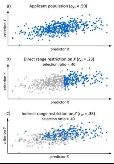
The predictive validity of X, or more precisely the correlation between a predictor X and a criterion of success Y, is a measure of the effectiveness of the selection. The higher the correlation between X and Y, the smaller the prediction error of the criterion values. However, the correlation between X and Y can only be obtained from the selected sample. Due to the selection itself, values of the criterion are not available for non-selected applicants. Figure 1 illustrates the loss of criterion data for DRR and IRR scenarios in the case of a continuous criterion variable. Figure 1a shows the complete data in which the (unrestricted) Pearson population correlation ρ is .50. Figure 1b and 1c illustrates the effects of selection on X and Z, respectively. The blue data points are the available selected sample, the gray data points represent the non-selected sample in which the values for Y are missing. In both scenarios, the selection ratio is .40, which is the ratio of the number of selected individuals to the number of applicants. Figure 1b shows that the top 40% of applicants are selected while 60% are not selected. Applicants with scores below a specific value of X are thus excluded from the sample. It is clear that scores of X in the selected sample are restricted in range. Consequently, the Pearson correlation coefficient obtained from the selected sample rXY = .23 is
significantly smaller than in the complete dataset. The correlation coefficient obtained from the selected sample underestimates the true population correlation.
Figure 1c shows an IRR scenario in which the loss of criterion data is based on another variable Z. In this example, Z is correlated with X and Y at .50, respectively, and the top 40% of applicants with respect to Z are selected. Consequently, the Pearson correlation coefficient obtained from the selected sample is rXY =
.38. The effect on correlations due to selection on Z is typically weaker than in the case of selection on X (Sackett & Yang, 2000). Levin (1972) showed that it is theoretically possible that selection on Z can increase rather than decrease the correlation coefficient when the correlations of Z with X and with Y become extreme. However, this effect is rarely encountered in real datasets, meaning that selection on Z can be expected to reduce the magnitude of the correlation coefficient (Linn et al., 1981).
Figure 1. An illustration of the loss of criterion data for direct and indirect range restriction scenarios in the case of a continuous criterion variable.
A closer look at the problem shows that the effect on the Pearson correlation coefficient does not stem directly from the restriction in range of X, but as a result of the reduction of the sample variances of X and Y as well as by the reduction of the sample covariance between X and Y in the selected sample. The problem arises from the formula of the Pearson correlation coefficient (Equation 1). The reduction of rXYis given as
the reduction in the sample covariance (the numerator) relative to the reduction in the product of the sample standard deviations sX and sY (the denominator).
,
∙ (1)
Next, we look at direct and indirect range restriction scenarios and the loss of criterion data in the case of a dichotomous criterion variable. So far only a few studies have focused on range restriction correction in the case of a dichotomous criterion variable (Bobko, Roth, &
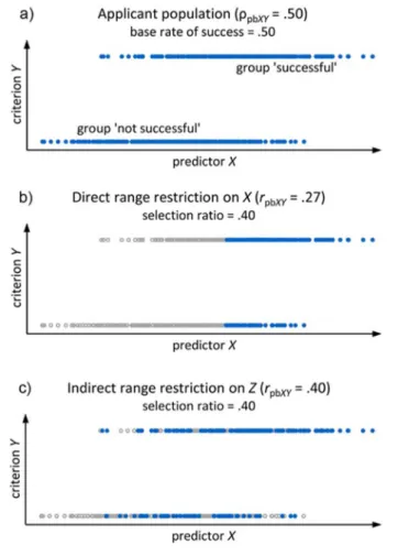
Bobko, 2001; Pfaffel, Kollmayer, et al., 2016; Raju, Steinhaus, Edwards, & DeLessio, 1991). Figure 2 shows that the criterion Y is divided into two groups (‘not successful’ and ‘successful’). The correlation coefficient used to express the relationship between a continuous and a naturally dichotomous variable is the point-biserial correlation coefficient (Ulrich & Wirtz, 2004), which is calculated by
(2) where M1 and M0 are the mean values of the continuous variable X for the two groups p (‘not successful’, Y = 0) and q (‘successful’, Y = 1), and sX is the standard deviation of the continuous variable X. Figure 2a shows the complete data in which the unrestricted point-biserial correlation coefficient ρ is .50. Figures 2b and 2c illustrate the effects on the point-biserial correlation coefficient due to selection on X and Z. In both scenarios, the selection ratio is 40%. In a DRR scenario, as shown in Figure 2b, applicants with scores below a specific value of X have been excluded from the sample. Consequently, obtained from the selected sample is .27. Figure 2c shows an IRR scenario in which the top 40% applicants with respect to Z have been selected; Z is correlated with X and Y at .50, respectively. In the case of IRR, we obtain a value for
of .40.
Range restriction in the case of a dichotomous criterion variable is similar to range restriction scenarios in the case of a continuous one. However, a very important factor that has to be considered additionally is the base rate of success BR (Abrahams, Alf, & Wolfe, 1971; Pfaffel, Kollmayer, et al., 2016). The BR is the percentage of applicants who would be successful on the criterion if there were no selection, and is calculated by dividing the number of successful individuals by the number of applicants. The BR ranges from 0 to 1, or from 0% to 100%. For example, if all applicants were to be admitted to a study program and 50% percent of them complete this program, then the BR is 50%. In our examples in Figure 2, we used a BR of 50%. The BR is closely related to the effectiveness of the selection, because a selection is considered effective when the percentage of successful applicants (in the selected sample) is higher than the BR, i.e. when the selected applicants are more frequently successful than would be
Figure 2. An illustration of the loss of criterion data for direct and indirect range restriction scenarios in the case of a dichotomous criterion variable.
the case by random chance. It is not surprising that when the BR is high, the probability of gaining an effective selection is low. In such a case, the incremental predictive validity of additional and resource-intensive selection methods should be examined. Thus, the BR also plays a role in assessing the efficiency of a selection method.
Unfortunately, the BR is unknown in the case of selection and thus the unbiased information about the proportion of successful individuals in the applicant population. We can only obtain the success rate from the selected sample, which is a biased estimator for the BR. The success rate is the number of successful individuals divided by the number of selected applicants. In Figures 2b and 2c, the success rate is 75%. This success rate is higher than the BR, because the relationship between predictor and criterion is positive. Hence, more applicants who would be successful have been selected.
In addition to the range restriction effect, the magnitude of the observed (restricted) point-biserial correlation coefficient is also affected by variance-restriction due to unequal p-q split (Kemery, Dunlap, & Griffeth, 1988). The variance of a dichotomous variable is the product of p and q with a maximum value of .25 at p = q = .50. If p does not equal q, the variance will be less than .25. Consequently, rpb decreases as p and q move away from .50, and increases as p and q move towards .50. The two effects can sometimes act in opposite directions. For example, assume that ρ is positive, the BR is .10, and after selection, the observed success rate is .60. Because .60 is closer to 0.50 than 0.10, the variance of the dichotomous variable in the selected sample is higher than in the population, and this consequently leads to an increase in rpb. In such a case, rpb decreases due to range restriction and increases due to the p-q split. Despite range restriction, it is conceivable that rpb is not much smaller than ρ because of the combination of the two effects. Therefore, correction methods for range restriction must take into account the effect of the p-q split in the case of a dichotomous criterion variable.
Approaches to correcting for direct and indirect range restriction scenarios
Researcher have proposed two approaches to correct correlations for direct and indirect range restriction scenarios. The traditional approach is to apply the correction formulas presented by Thorndike (1949). The formulas correct the Pearson correlation coefficient for univariate direct and indirect range restriction scenarios for continuous variables. They were derived within the framework of maximum likelihood estimation under the assumptions of multivariate normality, linearity between X and Y, and homoscedasticity. In the psychometric literature, it is well documented that corrected Pearson correlations are less biased than uncorrected correlations over a wide range of assumption violations (Greener & Osburn, 1979; Gross & Fleischman, 1983; Holmes, 1990; Linn, 1983; Linn et al., 1981; Ree et al., 1994). The corrected Pearson correlations are always higher than the uncorrected correlations. The formulas include only the variables X and Y, or X, Y, and Z, where X and Z must have no missing values. Covariates that could potentially contribute to the prediction of Y are not considered.
The modern approach is to view the selection mechanism as a missing data mechanism (Mendoza, 1993; Pfaffel, Kollmayer, et al., 2016; Pfaffel, Schober, et
al., 2016; Wiberg & Sundström, 2009). Rubin (1976) identified three missing data mechanisms, according to the underlying cause of missing data. These mechanisms are important since they are necessary assumptions for the missing data methods: Missing completely at random (MCAR) means the probability of missing values of Y is unrelated to other measured variables and to the values of Y itself. Missing at random (MAR) means the probability of missing values of Y is related to other measured variables, but not related to the values of Y itself. Missing not at random (MNAR) means the probability of missing values of Y is related to the values of Y itself, even after controlling for other variables. The missing data mechanism in both range restriction scenarios (DRR and IRR) is missing at random (MAR) because the missing values depend either on X or Z, but not on the values of Y itself (Pfaffel, Schober, et al., 2016).
The missing data approach has several advantages over the correction formulas: 1) This approach no longer requires a distinction between DRR and IRR to be made in applying the correction because both scenarios are considered to be MAR and the same techniques can be used to correct for both range restriction scenarios. 2) State-of-the-art missing data techniques such as full information maximum likelihood and multiple imputation can handle multivariate datasets with multiple covariates and 3) can also handle different types of predictor and criterion variables (e.g., dichotomous, unordered and ordered categorical, continuous). Pfaffel, Kollmayer, and colleagues (2016) showed that the correction using multiple imputation by chained equations is more accurate than Thorndike’s (1949) correction formulas when the criterion variable is dichotomous, especially in the case of IRR. 4) In contrast to Thorndike’s formulas, covariates – but not the selection variable – may have some missing values (missing values in the selection variable is MNAR). However, no empirical studies have been presented, which investigate the effect of covariates with missing values on the accuracy of the correction.
Methodologists currently regard full information maximum likelihood and multiple imputation as state of the art when dealing with missing data. Techniques such as listwise or pairwise deletion, arithmetic mean imputation, single regression imputation, or single EM imputation are no longer considered state-of-the-art because they have potentially serious drawbacks (Enders, 2010). For example, arithmetic mean
imputation imputes values that fall directly on a horizontal line. Consequently, the correlations between imputed values and other variables are zero for the subset of cases with imputed values. Arithmetic mean imputation attenuates correlations and covariances. In single regression imputation, the imputed values fall directly on the (straight) regression line, which overestimates correlations and covariances. This under- and overestimation of correlations is present under any missing data mechanism, including MCAR, and increases as the missing data rate increases (Enders, 2010). In addition, single imputation techniques attenuate standard errors. Neither state-of-the-art technique, full information maximum likelihood and multiple imputation, suffers from the problems mentioned for deletion of incomplete cases and single imputation techniques (Enders, 2010).
Full information maximum likelihood (FIML) is a technique of finding population parameters by maximizing the log-likelihood function that has the highest probability of producing the data of a certain sample. FIML requires the missing data mechanism to be either MAR or MCAR. Finding the parameter values that maximize the log-likelihood function is possible with iterative optimization algorithms such as expectation maximization (EM) algorithms (Dempster, Laird, & Rubin, 1977; Meng & Rubin, 1993). In the social and behavioral sciences, population data is commonly assumed to be multivariate normally distributed (Enders, 2010). Dealing with identically distributed variables is straightforward and many software packages can handle missing values under the condition of multivariate normality. FIML estimation with non-identically distributed variables in multivariate datasets is much more complicated, for example in logistic regression analysis. FIML with complex multivariate incomplete data is typically only possible with structural equation modeling (SEM) software, e.g. Mplus (Muthén & Muthén, 2015), or the lavaan package for R Statistics (Rosseel, 2012). For a detailed description of likelihood-based techniques, see Little and Rubin (2002), or for a less technical description see Enders (2010).
Multiple imputation (MI), proposed by Rubin (1978), is another state-of-the-art technique for handling missing values that allows the data analyst to use statistical methods designed for complete data. In contrast to FIML, MI creates plausible estimates for the missing values. MI and FIML make the same
assumptions regarding the missing data mechanism (MAR or MCAR), their estimators have similar statistical properties (e.g., consistency, asymptotic normality), and they frequently produce equivalent results (Enders, 2010; Graham, Olchowski, & Gilreath, 2007). A multiple imputation analysis consists of three distinct steps: the imputation phase, the analysis phase, and the pooling phase. The imputation phase creates m complete datasets (e.g., m = 20 imputations) based on one dataset with missing values. Each of these m complete datasets contains different plausible estimates of the missing values, but the observed values are identical. In contrast to a single imputation technique, the created m complete datasets reflect the uncertainty of the missing data. Thus, the imputed values do not fall on the regression line. Consequently, MI does not attenuate correlations and covariances. In the analysis phase, each complete dataset is analyzed with conventional statistical methods, e.g. m correlation analyses. Finally, the pooling phase combines the m parameter estimates into a single set of parameters, e.g. m correlation coefficients are combined into one pooled value. The pooled parameter values are typically the arithmetic average of the m estimates generated in the analysis phase (Rubin, 2004). Analyzing and pooling a large number of imputed datasets sound laborious, but modern MI software packages automate this procedure. Handling incomplete multivariate normal data is possible with the data augmentation algorithm (Schafer, 1997; Tanner & Wong, 1987). A general multiple imputation technique, which can handle incomplete datasets with not necessarily normal or non-identically distributed variables is multivariate imputation by chained equations (MICE), also known as fully conditional specification (FCS) (Raghunathan, Lepkowski, van Hoewyk, & Solenberger, 2001; van Buuren, 2007, 2012). The MICE algorithm, for example, is implemented in the R software package mice (van Buuren & Groothuis-Oudshoorn, 2011).
The multivariate imputation model is specified on a variable-by-variable basis by a set of conditional densities, one for each incomplete variable (van Buuren & Groothuis-Oudshoorn, 2011). In the case of an incomplete dichotomous variable such as our example in Figure 2, multiple imputation is possible using a logistic regression model, which incorporates the parameter uncertainty (Pfaffel, Kollmayer, et al., 2016; van Buuren, 2012). Typically, all variables or many variables in the dataset are part of the imputation model used to generate the plausible estimates of the missing
values. Because MI clearly separates the imputation and the analysis phase, the analysis model can differ from the imputation model. Therefore, the plausible estimates contain information on variables that might not be included in the analysis model. However, the imputation model has to be more general then the analysis model. For example, a common source for incompatibility occurs when the analysis model contains interactions and non-linearities, but the imputation model did not. Recent simulation studies show that correction for DRR and IRR with full information maximum likelihood or multiple imputation by chained equations is equally or more accurate compared to Thorndike’s (1949) correction formulas in the case of multivariate normality (Pfaffel, Schober, et al., 2016) and in the case of an artificially or a naturally dichotomous criterion variable (Pfaffel, Kollmayer, et al., 2016). Especially in the case of IRR, correction with a missing data technique is more precise and therefore more efficient than the formulas. Full information maximum likelihood and multiple imputation by chained equations produce equal parameter estimates. Because of these empirical findings and the advantages mentioned above, we recommend the use of missing data techniques to correct for range restriction.
Standard error of correlations corrected for range restriction
Estimating the standard error and confidence intervals of correlation coefficients in the case of missing data is often much more complex than with complete datasets. In this section, we first give a brief overview of calculating the standard error of correlation coefficients in the case of complete samples and in the case of missing data. Next, we present some approaches for estimating the standard error of correlation coefficients corrected for direct and indirect range restriction scenarios. Finally, we show that multiple imputation allows for calculating the standard error and confidence intervals of correlation coefficients very similar to complete datasets.
In statistics, it is well known that an unbiased estimator converges in probability to the true quantity being estimated as the sample size goes to infinity (property of consistency). This means that the sampling error of a sample parameter becomes smaller and smaller as the sample size increases, and is zero when the sample size is infinitely large. Conversely, if the sample size decreases, then the sampling error of the estimate
increases, making the estimation less precise. A common measure of the variability of the sampling distribution is the standard error SE, which is often used for calculating confidence intervals for a parameter estimate in hypothesis testing. A larger standard error is less likely to reject the null hypothesis. The sampling distribution of the Pearson correlation coefficient (Equation 1) is quite complex even under bivariate normality, and is a negatively biased estimator of ρ (Olkin & Pratt, 1958). However, this bias is small and decreases as the sample size increases. Thus, the true SE is not easy to calculate and only valid when the underlying assumptions are fully met. For complete data analysis, Kendall and Stuart (1977) proposed an approximation of SE of the sample Pearson correlation coefficient in samples with size N:
≈ 1
√ 1 (3)
Equation 3 shows that the SE of depends on the sample size and on the value of itself. Consequently, with the same sample size, a stronger correlation can be estimated more precisely than a weaker one. The procedure for examining the statistical significance and the asymmetric confidence interval of is to transform into a Fisher z-value with the associated standard error (Fisher, 1915):
!"#$%& ' √ 31 (4) As we can see, this standard error depends only on the sample size. Fisher’s z-transformation is necessary because the sampling distribution of rXY is skewed and correlation coefficients are only supported on the bounded interval [-1,1]. An asymmetric sampling distribution leads to asymmetric confidence intervals. Fisher’s z-transformation can also be applied to the point-biserial correlation coefficient because rpb is mathematically equivalent to the Pearson correlation coefficient.
Next, we want to show what happens to the SE in the case of range restriction, i.e. in the case of missing values. Many researchers have demonstrated that the SE of a corrected Pearson correlation coefficient is larger than for the uncorrected correlation coefficient (Bobko & Rieck, 1980; Mendoza, 1993; Millsap, 1989; Raju & Brand, 2003). The increase in the magnitude of SE can be explained by considering two circumstances: First,
the correlation coefficient is measured in a subsample with sample size ) ≤ , where ) is the size of the selected sample. As shown in Equation 3 and 4, the magnitude of the standard error is approximately inversely proportional to the square root of the sample size. Second, the population correlation estimate must include the uncertainty caused by the proportion of missing values. Consequently, the magnitude of the standard error increases by applying corrections for range restriction.
Bobko and Rieck (1980) presented a large sample estimator for the standard error of correlation coefficients corrected for a direct range restriction scenario. The estimator is the product of the standard error of the correlation coefficient obtained from the selected sample and a factor derived from Thorndike’s (1949) formula for direct range restriction scenarios. In case of indirect range restriction scenarios, a large sample estimator has been presented by Allan and Dunbar (1990), but this formula is very long and complicated. As shown for complete datasets, Fisher’s z-transformation can be applied to calculate the confidence interval of correlation coefficients. However, Mendoza (1993) showed that Fisher’s z-transformation cannot directly applied to correlations corrected for direct and indirect range restriction scenarios (assumption MAR), and proposed additional correction terms to the Fisher’s z -transformation. Admittedly computers allow to easily calculate these formulas. However, this examples show that deriving the sampling distribution under the framework of maximum likelihood estimation, especially in the case of missing data, often leads to complex problems relatively quickly. In summary, it can be ascertained that deriving the sampling distribution of the sample correlation coefficient under the framework of maximum likelihood estimation is very complex or maybe sometimes impossible in the case of (non-normal) multivariate distributions with missing data.
In contrast, calculating the standard error using multiple imputation is relatively straightforward. A major advantage is that conventional statistical procedures to calculate the standard error can be applied to the m complete datasets. Moreover, the correlation is calculated based on the total sample size N, and therefore making Fisher's z-transformation much more accurate. Multiple imputation standard errors combine two sources of uncertainty regarding the parameter estimate (Little & Rubin, 2002): The uncertainty within an imputation (the within-imputation variance), and the
uncertainty between the m imputations (the between-imputation variance). The Fisher’s z standard error of one of the m complete datasets represents the uncertainty of the data. The increase in Fisher’s standard error in the case of missing data results from the between-imputation variance. The parameter estimates and the standard errors can be combined by Rubin’s rules (Rubin, 2004). The Appendix shows the equations for computing the estimate of the correlation coefficient, its associated standard error, and the confidence interval for multiple imputed datasets. However, software packages typically implement these procedures, so there is usually no need to compute parameter estimates by hand.
As mentioned above, multiple imputation and full information maximum likelihood make the same assumptions and have similar statistical properties. The statistical theory underlying these techniques is based partly on large-sample approximations. However, this statement must be restricted because the two missing data techniques differ in their performance in the case of small sample sizes. Simulation studies show that maximum likelihood estimation is inadequate for small or moderate sample sizes and is likely to result in biased estimates (Graham & Schafer, 1999; Little & Rubin, 1989). The findings suggest that multiple imputation performs more efficiently with small samples. Graham and Schafer (1999, p. 26) pointed out that “limitations of analysis with small sample size lie in the small sample size itself, not with the multiple-imputation procedure”. This finding is fundamental for empirical evaluation studies of the predictive validity of selection methods. On the one hand, it supports the use of multiple imputation in small or moderate samples. On the other hand, it makes clear that multiple imputation cannot compensate for having a small number of applicants or small selection ratios. However, multiple imputation allows for the most effective usage of all the data that have been collected.
Therefore, we suggest using a Bayesian multiple imputation technique such as multiple imputation by chained equations to overcome the range restriction problem in small or moderate samples. So far, simulation studies investigating the accuracy of this missing data technique when the sample size is small or moderate are lacking. Additionally, little is known about the correctness of the multiple imputation standard error in the case of range restriction. Our intention is to close these research gaps. The accuracy of the corrected
correlation coefficient and of the multiple imputation standard error are important considerations for researchers and evaluators. Thus, our empirical findings will help to increase understanding of the circumstances (e.g. sample size, selection ratio, true population correlation) under which range restriction corrections are appropriate.
Purposes of this study
The first purpose is to examine the accuracy of the population correlation estimates by using multiple imputation by chained equations in terms of small and moderate sample sizes for direct and indirect range restriction scenarios, and for continuous and naturally dichotomous criterion variables. The second purpose is to examine the accuracy of the associated multiple imputation standard error.
Method
We conducted several Monte Carlo simulations to examine the accuracy of the proposed missing data approach and the sampling distribution of the multiple imputation standard error under different model conditions. Multivariate data were simulated in order to investigate four scenarios: DRR and IRR scenarios with a continuous criterion variable, and DRR and IRR scenarios with a naturally dichotomous criterion variable. Additionally, three factors (continuous criterion) and four factors (dichotomous criterion) that affect the accuracy of the correction as well as the sampling distribution of the standard error were systematically manipulated.
Factor 1: Total sample size, N. Multiple imputation was developed under the framework of large sample theory. In contrast to maximum likelihood estimation, multiple imputation seems to promise a more accurate correction when the sample size is small or moderate. As shown in Equations 3 and 4, sample size also affects the standard error of the correlation coefficient. Therefore, sample size is a very important factor in studying asymptotic estimates. Two different sample sizes were investigated: a small sample with size N = 50, and a moderate sample with size of N = 100.
Factor 2: Population correlation, + and +,- . The effect of the population correlation on the accuracy of
1 In a preliminary experiment, we also tested a selection ratio of 10%, but frequent convergence problems led to invalid estimates. In
the correction has been documented in a number of empirical studies (Duan & Dunlap, 1997; Pfaffel, Kollmayer, et al., 2016; Pfaffel, Schober, et al., 2016). The correction to the correlation coefficient becomes more precise as the population correlation increases. This effect is valid for DRR and IRR and for continuous and dichotomous criterion variables. As shown in Equation 3, the standard error of the correlation coefficient depends on the magnitude of the correlation coefficient itself and decreases as the correlation coefficient increases. Hence, in the present study, we investigated three levels of ρ and ρ .20, .40, and .60. According to Cohen’s (1988) classification of correlation coefficients in the social sciences, these values represent a small, medium, and large association between predictor and criterion, i.e. a small, medium, and large predictive validity.
Factor 3: Selection ratio, SR. The selection ratio is the ratio of the number of selected applicants to the total sample size N. The selection ratio directly affects the proportion of missing values in the criterion variable, and therefore the accuracy of the correction. Correlation estimates become more biased and exponentially less precise when the selection ratio decreases (Pfaffel, Schober, et al., 2016). It is to be expected that this adverse effect increases, when sample sizes become small or moderate. Hence, in the present study, we investigated four levels of the selection ratio: 20%, 30%, 40%, and 50%. The smallest selection ratio of 20% corresponds to subsample sizes of n = 10 (N = 50) and n = 20 (N = 100). These two sample sizes have to be considered extremely small because on the one hand, 80% of the criterion values have been systematically excluded, and on the other hand, 10 and 20 observations are small even for complete data analysis1.
Factor 4: Base rate of success, BR. This factor was used in the case of a dichotomous criterion variable. As described above, the effect of range restriction and the effect of variance restriction can sometimes work in opposite directions when the p-q split is closer to .50 in the selected sample than in the unrestricted sample. Therefore, the effect of the BR is an especially relevant factor to investigate when the criterion variable is dichotomous. In the present study, we varied the BR at three levels: 20%, 50%, and 80%. These three levels represent a small, medium, and large proportion of
the case of a dichotomous criterion, Y was almost always constant in the subsample.
applicants who would be successful if there were no selection.
Monte Carlo simulation procedure
The Monte Carlo simulations were conducted using the program R (R Core Team, 2016) with 5,000 iterations for each factor combination of sample size, population correlation, selection ratio, and base rate of success. In the case of a continuous criterion variable, there were 2×3×4 = 24 factor combinations, while in the case of a dichotomous criterion variable, 2×3×4×3 = 72 factor combinations were investigated. For each of the four scenarios (DRR & IRR × continuous & dichotomous), a random sample with size N was generated from a multivariate distribution (see Data simulation) with a population correlation ρ or ρ between predictor X and criterion Y, and a base rate of success in the case of a dichotomous criterion variable. Then, we simulated the selection by isolating those n = N·SR cases with the highest values in X in the case of a DRR scenario, and in descending order by the third variable Z in the case of an IRR scenario. Values of Y for non-selected cases were converted into missing values. The selected samples created in this way with
) missing values in Y were used in applying the correction. Next, we used the R package mice (multivariate imputation by chained equations, Version 2.25, van Buuren & Groothuis-Oudshoorn, 2011) to generate m = 20 imputed datasets. Pfaffel, Kollmayer and colleagues (2016) showed that 20 imputations are sufficient for DRR and IRR corrections using multiple imputation by chained equations. We used the elementary imputation method ‘norm’ for the imputation of the continuous criterion variable, and the method ‘logreg’ for the imputation of the dichotomous criterion variable. Finally, the pooled correlation coefficients and the multiple imputation standard errors were calculated using Fisher’s z-transformation and Rubin’s (2004) rules for combining multiple imputation parameter estimates (for details, see the Appendix).
Pfaffel, Kollmayer, and colleagues (2016) reported problems (e.g. constancy of Y in the selected sample) in conducting a logistic regression analysis for some factor combinations, especially when the base rate of success and the population correlation were high and the selection ratio was small. They excluded selected samples (with minimum sample size of n = 50) with less than five observations in each of the two criterion groups. In the present study, the smallest n was 10 when
the total sample size N was 50 and the selection ratio .20. Requiring at least five observations in each criterion group means that only one p-q split of 50% in the selected sample is valid for n = 10. Thus, there would be no variability in the p-q split for this factor combination. Consequently, we weakened the prerequisite to at least three observations in each of the two criterion groups.
Data simulation
We simulated multivariate data for a) a normally distributed (continuous) criterion variable and b) for a naturally dichotomously distributed criterion variable. In simulating the multivariate data, we used the procedures presented in the studies by Pfaffel, Schober, et al. (2016) and Pfaffel, Kollmayer, et al. (2016).
a) Continuous criterion: We generated a bivariate (DRR) and a trivariate (IRR) standard normal distribution with Pearson population correlations between X and Y of .20, .40, and .60 using the mvrnorm function of the MASS package (Venables & Ripley, 2002). In the case of IRR, the Pearson correlations between Z and X, and Z and Y were varied continuously between .10 and .90. This continuous variation facilitates the aggregation of a parameter estimate over factors and factor levels (more specifically, it facilitates integration over a continuous interval of a parameter). Aggregating parameter estimates over other factors with only a few levels would lead to an underestimation of the variance of the parameter estimate, and therefore to a biased empirical sampling deviation.
b) Naturally dichotomous criterion: The distribution of a naturally dichotomous criterion variable is defined via the two proportions p and q, no underlying distribution exists. We generated bivariate (DRR) and trivariate (IRR) data where Y was naturally dichotomous, and X and Z were a mixture distribution of two uniform normal distributions, one normal distribution for each of the two criterion groups. Abrahams and colleagues (1971) also used this mixture distribution to develop the Taylor-Russell tables for dichotomous criterion variables. As shown in Equation 2, the magnitude of the point-biserial correlation coefficient depends on the mean difference in X (or in Z) between the two criterion groups. Therefore, we generated data with point-biserial population correlations between X and Y of .20, .40, and .60 based on the difference in mean for a given p-q split. In the case of IRR, we varied the differences in means and therefore Pearson correlations between Z and X, and Z and Y continuously between .10 and .90.
Analysis of the parameters
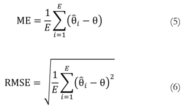
In order to investigate the accuracy of the missing data approach, we analyzed the residual distribution of the correlation estimates for each factor combination. The concept of accuracy provides quantitative information about the goodness of a parameter estimate and encompasses trueness and precision (Ayyub & McCuen, 2011). Trueness, which is also known as bias or systematic error, describes the distance of an estimated value to the true parameter value. Precision, which is also known as random error, describes the reproducibility of an estimated value. The mean error (ME) of the residuals is a measure of trueness, and the root-mean-square error (RMSE) of the residuals is a measure of precision. Let θ/ be the value of the parameter estimate and θ the true value of the parameter. The ME and the RMSE can be calculated by
ME 123θ/" θ4 5 "6 (5) RMSE 9123θ/" θ4 5 "6 (6)
where E is the number of the Monte Carlo experiments (E = 5,000 in the present study), and θ/" is the pooled correlation coefficient from the multiple imputation analysis. When the ME is close to zero, the parameter estimate is to be said unbiased. The smaller
the RMSE, the more precise the estimation, i.e. the higher the reproducibility of the estimated parameter value.
The multiple imputation standard error of the correlation coefficient (see Appendix Equation A8) is a theoretical (asymptotic) estimate of the sampling deviation of the sample correlation coefficient. The RMSE is a measure of the empirical sampling deviation of the sample correlation coefficient. In order to investigate the accuracy of the multiple imputation standard error, we compared its average value (over 5,000 Monte Carlo experiments) with the RMSE for each factor combination. When the difference between the theoretical and the empirical value of the multiple imputation standard error is close to zero, the theoretical value is an accurate measure of the true sampling distribution of the corrected sample correlation coefficient. When the theoretical value of the multiple imputation standard error is smaller than the empirical sampling deviation, the confidence intervals for the population correlation based on the multiple imputation standard error are smaller than they need to be.
Results
Continuous criterion variable
Table 1 summarizes the trueness and the precision of the correction for direct and indirect range restriction scenarios in the case of a continuous criterion variable across 5,000 Monte-Carlo experiments for each factor combination. For both the DRR and IRR scenarios, the correction of the Pearson correlation coefficient is negatively biased, whereby the bias tends to be smaller in the case of an IRR scenario. The bias is higher for a
Table 1. Mean error (ME) and root-mean-square error (RMSE, in parentheses) for a continuous criterion variable in the case of direct and indirect range restriction scenarios.
DRR IRR N SR ρ = .2 ρ = .4 ρ = .6 ρ = .2 ρ = .4 ρ = .6 50 0.2 -.075 (.499) -.157 (.506) -.178 (.466) -0.088 (.315) -0.117 (.312) -0.140 (.293) 0.3 -.056 (.403) -.100 (.389) -.100 (.332) -0.051 (.248) -0.074 (.239) -0.080 (.204) 0.4 -.035 (.333) -.067 (.308) -.067 (.249) -0.035 (.201) -0.047 (.187) -0.053 (.154) 0.5 -.022 (.273) -.041 (.249) -.043 (.190) -0.022 (.165) -0.032 (.154) -0.034 (.117) 100 0.2 -.053 (.391) -.083 (.368) -.098 (.316) -0.053 (.232) -0.068 (.224) -0.070 (.185) 0.3 -.031 (.303) -.047 (.273) -.056 (.218) -0.030 (.176) -0.037 (.161) -0.042 (.134) 0.4 -.021 (.242) -.031 (.219) -.035 (.163) -0.021 (.143) -0.023 (.125) -0.027 (.102) 0.5 -.012 (.199) -.021 (.175) -.022 (.126) -0.016 (.116) -0.013 (.099) -0.017 (.078)
Note. N … sample size of the applicant dataset, SR … selection ratio, ρ … population correlation between predictor and criterion, DRR … direct range restriction scenario, IRR … indirect range restriction scenario
small sample size of N = 50 than for a moderate sample size of N = 100, and increases as the selection ratio decreases and the true correlation coefficient between X and Y increases. The correction is more precise for moderate samples than for small ones and increases as the selection ratio increases. The precision of the correction increases as the true Pearson correlation coefficient between X and Y increases.
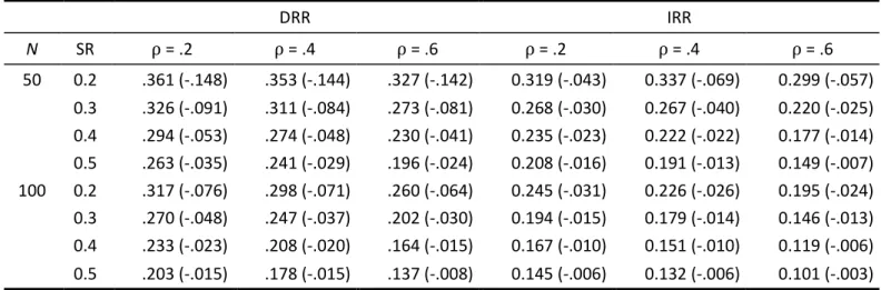
Table 2 summarizes the comparison of the multiple imputation standard error with the empirical sampling distribution for direct and indirect range restriction scenarios in the case of a continuous criterion variable across 5,000 Monte-Carlo experiments for each factor combination. The results show that the multiple imputation standard error tends to underestimate the sampling deviation of the sample correlation coefficient. This underestimation tends to be smaller in the case of an IRR scenario than for a DRR scenario. The difference between the multiple imputation standard error and the sampling deviation decreases as the selection ratio, the sample size, and the population correlation increase.
Naturally dichotomous criterion variable
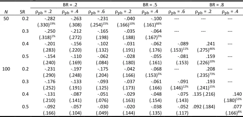
Table 3 summarizes the trueness and the precision of the correction for a direct range restriction scenario in the case of a naturally dichotomous criterion variable for each factor combination. However, for a number of factor combinations the number of Monte Carlo experiments was less than 5,000. More than 90% of selected samples did not meet the prerequisite of at least three observations in each criterion group, or there were
convergence problems with the logistic regression imputation. No selected sample met the prerequisite at a base rate of success (BR) of 80% and a true point-biserial correlation coefficient of .6. The superscripted numbers in Table 3 and 5 show the percentage of excluded samples. Results of the remaining Monte Carlo experiments show that the correction of the point-biserial correlation coefficient is negatively biased for factor combinations of sample size, true point-biserial correlation coefficient, and selection ratio when the base rate of success is 20% or 50%, but positively biased when the BR is 80%. As expected, the bias decreases as the selection ratio and the sample size increase. The effect of the direction of the true point-biserial correlation coefficient varied across different base rates of success: For a BR of 20%, the bias of the correction become smaller as ρ increases, but for a BR of 50%, bias increases as ρ increases. For a BR of 80%, too many data points are missing to assess the direction of the effect. The correction become more precise as the sample size, the selection ratio, and the true correlation
between predictor and criterion increase. Comparing the results of the same factor combinations across the three base rates of success to the extent allowed by the data reveals that the correction is most accurate when the BR is 50%. This indicates a non-linear relationship between base rate of success and accuracy.
Table 2. Average multiple imputation standard error and its absolute bias to the empirical sampling deviation (in parentheses) for a continuous criterion variable in the case of direct and indirect range restriction scenarios.
DRR IRR N SR ρ = .2 ρ = .4 ρ = .6 ρ = .2 ρ = .4 ρ = .6 50 0.2 .361 (-.148) .353 (-.144) .327 (-.142) 0.319 (-.043) 0.337 (-.069) 0.299 (-.057) 0.3 .326 (-.091) .311 (-.084) .273 (-.081) 0.268 (-.030) 0.267 (-.040) 0.220 (-.025) 0.4 .294 (-.053) .274 (-.048) .230 (-.041) 0.235 (-.023) 0.222 (-.022) 0.177 (-.014) 0.5 .263 (-.035) .241 (-.029) .196 (-.024) 0.208 (-.016) 0.191 (-.013) 0.149 (-.007) 100 0.2 .317 (-.076) .298 (-.071) .260 (-.064) 0.245 (-.031) 0.226 (-.026) 0.195 (-.024) 0.3 .270 (-.048) .247 (-.037) .202 (-.030) 0.194 (-.015) 0.179 (-.014) 0.146 (-.013) 0.4 .233 (-.023) .208 (-.020) .164 (-.015) 0.167 (-.010) 0.151 (-.010) 0.119 (-.006) 0.5 .203 (-.015) .178 (-.015) .137 (-.008) 0.145 (-.006) 0.132 (-.006) 0.101 (-.003)
Note. N … sample size of the applicant dataset, SR … selection ratio, ρ … population correlation between predictor and criterion, DRR … direct range restriction scenario, IRR … indirect range restriction scenario.
Table 4 shows the difference between the multiple imputation standard error of the estimate of the
point-biserial correlation coefficient and its empirical sampling deviation decreases as the sample size and selection ratio
Table 3. Mean error and root-mean-square error (in parentheses) for a naturally dichotomous criterion variable in the case of direct range restriction scenarios.
N SR BR = .2 BR = .5 BR = .8 ρ = .2 ρ = .4 ρ = .6 ρ = .2 ρ = .4 ρ = .6 ρ = .2 ρ = .4 50 0.2 -.282 (.330)19% -.263 (.308) -.231 (.254)15% -.040 (.166)10% -.100 (.161)66% --- --- --- 0.3 -.250 (.318)1% -.212 (.272) -.165 (.198) -.035 (.188) -.064 (.167)5% --- --- --- 0.4 -.201 (.283) -.156 (.220) -.102 (.132) -.031 (.191) -.062 (.176) -.089 (.153)11% .241 (.275)46% --- 0.5 -.154 (.240) -.110 (.169) -.062 (.084) -.028 (.180) -.055 (.161) -.081 (.153) .159 (.226)10% --- 100 0.2 -.231 (.290) -.197 (.248) -.175 (.204) -.042 (.166) -.068 (.153)5% --- .208 (.235)73% --- 0.3 -.176 (.252) -.133 (.191) -.093 (.125) -.037 (.173) -.061 (.166) -.091 (.146)12% .193 (.241)15% --- 0.4 -.131 (.210) -.087 (.141) -.051 (.076) -.029 (.163) -.048 (.154) -.075 (.143) .135 (.216) .140 (.180)53% 0.5 -.092 (.166) -.057 (.104) -.030 (.049) -.020 (.144) -.038 (.135) -.052 (.117) .092 (.184) .077 (.166)8%
Note. N … sample size of the applicant dataset, SR … selection ratio, BR … base rate of success, ρpb … population correlation between predictor
and criterion, --- … ≥80% of selected samples did not meet the prerequisite of at least three observations in each criterion group.
Table 4. Average multiple imputation standard error and its absolute bias to the empirical sampling deviation (in parentheses) for a naturally dichotomous criterion variable in the case of direct range restriction scenarios.
N SR BR = .2 BR = .5 BR = .8 ρ = .2 ρ = .4 ρ = .6 ρ = .2 ρ = .4 ρ = .6 ρ = .2 ρ = .4 50 0.2 .277 (-.021) .270 (-.057) .256 (-.057) .276 (.075) .268 (.044) --- --- --- 0.3 .266 (-.060) .249 (-.055) .213 (-.015) .264 (.048) .254 (.050) --- --- --- 0.4 .249 (-.056) .243 (-.041) .171 (-.011) .249 (.029) .237 (.029) .221 (.030) .252 (.016) --- 0.5 .231 (-.043) .198 (-.030) .142 (-.004) .231 (.018) .216 (.018) .194 (.020) .245 (.013) --- 100 0.2 .240 (-.064) .223 (-.043) .200 (-.016) .238 (.055) .232 (.061) --- .234 (.028) --- 0.3 .220 (-.053) .189 (-.030) .140 (-.004) .222 (.030) .214 (.036) .205 (.036) .230 (-.003) --- 0.4 .197 (-.039) .159 (-.018) .105 (-.002) .202 (.017) .192 (.020) .178 (.023) .222 (-.003) .209 (.041) 0.5 .176 (-.025) .135 (-.010) .088 (-.001) .183 (.012) .167 (.012) .143 (.010) .209 (-.008) .203 (.034)
Note. N … sample size of the applicant dataset, SR … selection ratio, BR … base rate of success, ρpb … population correlation between predictor
increase. The effect of the true point-biserial population correlation is not clear: For a BR of 20% only, this difference tends to decrease as the true population correlation increases. For a BR of 20%, the multiple imputation standard error tends to underestimate the sampling deviation; for base rates of success of 50% and 80%, the multiple imputation standard error tends to overestimate the sampling deviation for all combinations of sample size, selection ratio, and true point-biserial population correlation.
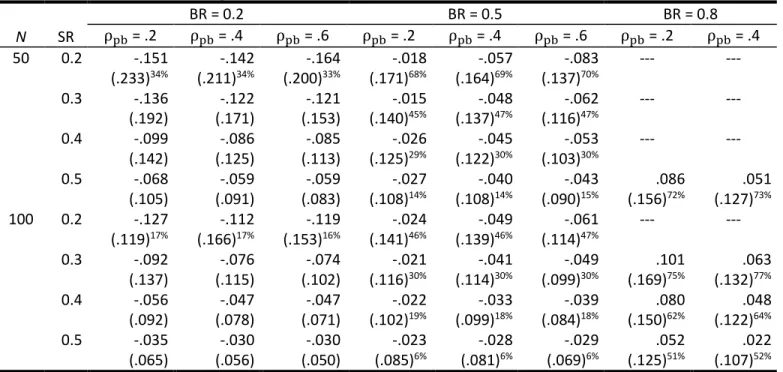
Table 5 summarizes the trueness and precision of the correction for an indirect range restriction scenario in the case of a naturally dichotomous criterion variable for each factor combination. The results show a similar pattern as the correction for a direct range restriction scenario. The correction of the point-biserial
correlation coefficient is negatively biased for factor combinations of sample size, true point-biserial correlation coefficient, and selection ratio when the base rate of success is 20% or 50%, but positively biased when the BR is 80%. The bias decreases as the selection ratio and the sample size increase. The correction becomes more precise as the sample size, the selection ratio, and the true point-biserial
correlation coefficient between predictor and criterion increase. Similar to DRR, the correction is least biased
when the BR is 50%. In contrast to DRR, the
correction is not most precise for a BR of 50%. For a moderate sample size of N = 100, the precision of the correction tends to decrease as the base rate of success increases.
Table 6 shows the results for the accuracy of the multiple imputation standard error of the estimate of the point-biserial correlation coefficient for a dichotomous criterion variable in the case of an indirect range restriction scenario. The difference between the multiple imputation standard error and its empirical sampling deviation decreases as the sample size and the selection ratio increase. For a BR of 20% and 50%, this difference decreases as the true point-biserial population correlation increases, but the effect for a BR of 80% is not clear.
Discussion
Statistical problems in estimating the predictive validity of a selection method become worse when the number of applicants in the unrestricted dataset is moderate or small because statistical estimates are only based on a subsample of applicants. In this paper, we proposed using the state-of-the-art missing data approach multiple imputation by chained equations to correct correlations for direct and indirect range
Table 5. Mean error (ME) and root-mean-square error (RMSE, in parentheses) for a naturally dichotomous criterion variable in the case of indirect range restriction scenarios.
N SR BR = 0.2 BR = 0.5 BR = 0.8 ρ = .2 ρ = .4 ρ = .6 ρ = .2 ρ = .4 ρ = .6 ρ = .2 ρ = .4 50 0.2 -.151 (.233)34% -.142 (.211)34% -.164 (.200)33% -.018 (.171)68% -.057 (.164)69% -.083 (.137)70% --- --- 0.3 -.136 (.192) -.122 (.171) -.121 (.153) -.015 (.140)45% -.048 (.137)47% -.062 (.116)47% --- --- 0.4 -.099 (.142) -.086 (.125) -.085 (.113) -.026 (.125)29% -.045 (.122)30% -.053 (.103)30% --- --- 0.5 -.068 (.105) -.059 (.091) -.059 (.083) -.027 (.108)14% -.040 (.108)14% -.043 (.090)15% .086 (.156)72% .051 (.127)73% 100 0.2 -.127 (.119)17% -.112 (.166)17% -.119 (.153)16% -.024 (.141)46% -.049 (.139)46% -.061 (.114)47% --- --- 0.3 -.092 (.137) -.076 (.115) -.074 (.102) -.021 (.116)30% -.041 (.114)30% -.049 (.099)30% .101 (.169)75% .063 (.132)77% 0.4 -.056 (.092) -.047 (.078) -.047 (.071) -.022 (.102)19% -.033 (.099)18% -.039 (.084)18% .080 (.150)62% .048 (.122)64% 0.5 -.035 (.065) -.030 (.056) -.030 (.050) -.023 (.085)6% -.028 (.081)6% -.029 (.069)6% .052 (.125)51% .022 (.107)52%
Note. N … sample size of the applicant dataset, SR … selection ratio, BR … base rate of success, ρpb … population correlation between predictor
restriction scenarios when the sample size is small or moderate. Approaches to overcoming the range restriction problem, including multiple imputation techniques, have been developed within the framework of large sample theory. However, some findings on the comparison between maximum likelihood and multiple imputation suggest that multiple imputation is more efficiently with small samples. Additionally, correction methods have been widely studied for continuous criterion variables but not for dichotomous ones. Therefore, the primary purpose of this research was to examine the accuracy of correlation coefficients corrected for range restriction scenarios using multiple imputation by chained equations in small or moderate samples and for continuous and dichotomous criterion variables. To the best of our knowledge, no empirical studies so far have investigated the accuracy of the multiple imputation standard error of the population correlation estimate in the case of direct (DRR) and indirect (IRR) range restriction scenarios. Therefore, the second purpose of this study was to examine the accuracy of the multiple imputation standard error of the population correlation estimate. We conducted Monte Carlo simulations to accomplish both purposes for four scenarios: a DRR and an IRR scenario with a continuous and a dichotomous criterion variable. Sample size,
selection ratio, true population correlation, and base rate of success were systematically varied in an experimental design.
In the case of a continuous criterion variable, the corrected Pearson correlation coefficient systematically underestimated the true correlation between predictor and criterion for both direct and indirect range restriction scenarios, especially when the selection ratio was small with 20% selected applicants. The correction was more precise for moderate samples than for small samples and gradually increased as the selection ratio and the true correlation coefficient increased. Our results are consistent with the findings of the simulation studies by Chan and Chan (2004), who investigated Thorndike’s correction formula for a selection scenario on X (DRR). The extent of this bias is similar for both approaches, e.g. for N = 100, SR = .2, and ρ = .2: -.053 and -.059 (p. 374). This means that the underestimation of the correlation coefficient due to range restriction cannot be fully corrected in either approach. The multiple imputation standard error of the corrected correlation coefficient tended to be smaller than the empirical sampling deviation, which means that confidence intervals for the population correlations are smaller than they should be. This bias was lower for moderate than
Table 6. Average multiple imputation standard error and its absolute bias to the empirical sampling deviation (in parentheses) for a naturally dichotomous criterion variable in the case of indirect range restriction scenarios.
N SR BR = .2 BR = .5 BR = .8 ρ = .2 ρ = .4 ρ = .6 ρ = .2 ρ = .4 ρ = .6 ρ = .2 ρ = .4 50 0.2 .248 (-.020) .237 (-.006) .218 (.002) .247 (.033) .235 (.041) .208 (.052) --- --- 0.3 .221 (-.019) .208 (-.006) .185 (.007) .225 (.036) .210 (.035) .182 (.039) --- --- 0.4 .196 (-.004) .181 (-.004) .156 (.013) .206 (.032) .192 (.027) .162 (.029) --- --- 0.5 .177 (.002) .162 (.008) .137 (.014) .189 (.022) .175 (.017) .146 (.020) .195 (.003) .172 (.018) 100 0.2 .198 (-.017) .183 (.013) .162 (-.003) .201 (.037) .187 (.034) .160 (.027) --- --- 0.3 .163 (-.007) .147 (.004) .122 (.003) .178 (.032) .165 (.027) .140 (.022) .183 (.002) .162 (.014) 0.4 .139 (.002) .122 (.002) .099 (.005) .160 (.022) .147 (.019) .121 (.015) .173 (.013) .152 (.013) 0.5 .124 (.003) .108 (.002) .087 (.005) .142 (.016) .130 (.015) .105 (.010) .163 (.024) .146 (.019)
Note. N … sample size of the applicant dataset, SR … selection ratio, BR … base rate of success, ρpb … population correlation between predictor