Online Full Text



Abstract—A hybrid approach is presented here, based on the

design of experiments (DOE) methodology and on the artificial neural networks (ANNs) for the modeling of the three component cutting force system in longitudinal turning of AISI D6 tool steel specimens. The selected inputs of the ANN model are the cutting speed, the feed rate and the depth of cut. The outputs are the three components of the cutting force, namely the feed force (Fz), the radial thrust force (Fx) and the tangential (main) cutting force (Fy). Twenty seven experiments were conducted having all different combinations of cutting parameter values. The three cutting parameters have three levels each one. The neural network toolbox of Matlab software was used to create, train, and test the ANN. A feed-forward back-propagation neural network (FFBP-NN) was selected to simulate the data. The results obtained indicate that the proposed modeling approach could be effectively used to predict the three component cutting force system during turning of AISI D6 tool steel, thus supporting decision making during process planning and providing a possible way to avoid time- and money-consuming experiments.

Index Terms—neural networks, turning, cutting forces, D6

tool steel

I. INTRODUCTION

urning is a type of material processing operation where a cutting tool is used to remove unwanted material to produce a desired product and it is generally performed on either conventional or computer numerically controlled (CNC) lathes. In recent decades, considerable improvements were achieved in turning, enhancing machining of difficult-to-cut materials and resulting in improved machinability (better surface finish and lower cutting forces) [1].

Manuscript received November 16, 2011; revised March 14, 2013. N. M. Vaxevanidis is with the Department of Mechanical Engineering Educators, School of Pedagogical & Technological Education (ASPETE), N. Heraklion, Athens, Greece (e-mail: [email protected])

J. D. Kechagias is with the Department of Mechanical Engineering, Technological Educational Institute of Larissa, Larissa, 41110 Greece (phone: 0030-2410-684322; e-mail: [email protected]).

N. A. Fountas is with the Department of Mechanical Engineering Educators, School of Pedagogical & Technological Education (ASPETE), N. Heraklion, Athens, Greece (e-mail: [email protected])

D. E. Manolakos is with the School of Mechanical Engineering, National Technical University of Athens (NTUA) Greece (e-mail: [email protected])

Cutting force estimation and modeling are of major importance for the metal cutting theory. There is a great number of inter-related parameters that affect the cutting forces, such as operational parameters, cutting tool geometrical characteristics and coatings, etc; therefore the development of a proper model is a quite difficult task [2]. Although that an enormous amount of related data is available in machining handbooks, the majority of these data attempt to define the relationship between only a few of the various cutting parameters whilst keeping the other parameters fixed [3].

ANNs are one of the most powerful computer modeling techniques, currently being used in many fields of engineering for modeling complex relationships which are difficult to describe with physical models. ANNs have been extensively applied in modeling many metal-cutting operations either conventional (turning, milling, grinding) or unconventional (EDM, AWJM, etc) [3-8].

This paper aims at developing a model for cutting force estimation and optimization based on ANNs.

II. ARTIFICIAL NEURAL NETWORKS OVERVIEW REVIEW STAGE Τhe origin, the development and the mathematical details of implementation of the ANNs can be found in a number of excellent reference works/textbooks, see for example [9]; therefore they are not discussed in the following sections.

III. EXPERIMENTAL PROCEDURES

The experimental procedure was designed using Taguchi method [10], which uses an orthogonal array to study the entire parametric space with performing only a limited number of experiments. Α three parameter design was selected with each parameter having three levels (Table I). The standard L27 (313) orthogonal array was used (Table II) [10]. Note, that the selection of L27 was done by taking into account preliminary experimentation in which strong interactions among cutting parameters were noticed.

The three turning parameters (factors) considered in this study are: cutting speed (S, m/min), feed rate (f, mm/rev) and depth of cut (a, mm). The kinematics of the longitudinal turning process is illustrated in Fig.1. A 3D cutting force system was considered according to standard theory of oblique cutting [2].

Three Component Cutting Force System

Modeling and Optimization in Turning of AISI

D6 Tool Steel Using Design of Experiments and

Neural Networks

Nikolaos M. Vaxevanidis, John D. Kechagias, Nikolaos A. Fountas, Dimitrios E. Manolakos

T

Columns 1, 2, and 5 of Table II are assigned to cutting speed (m/min), feed rate (mm/rev), and depth of cut (mm), while the rest columns left vacant. The selection of this orthogonal array have been done taking in account previous preliminary experimental work that shows strong interactions between cutting parameters.

Turning experiments were conducted using a Kern Model D18L conventional lathe. A SECO® coated tool insert, coded as TNMG 160404 – MF2 with TP 2000 coated grade, was used during the present series of experiments. The tool has triangular shape with cutting edge angle, Kr 55ο. Note that the accurate determination of cutting forces is essential for processes performance, for the evaluation of machining accuracy as well as for tool wear studies and for developing machinability criteria [11].

The test material was a tool steel supplied from Uddelholm Greece s.a with commercial name Sverker3®. It is a high-carbon (2.05%), high-chromium (12.7%) tool steel alloyed with tungsten (1.1%) identical to AISI D6 grade, with hardness 240 HB. The test specimens were in the form of bars; 43 mm in diameter and a tailstock was used.

Cutting force components were measured using a

three-TABLEI PARAMETER DESIGN.

Parameters Units Levels 1 2 3 A Cutting speed (S) m/min 115 81 57 B Feed rate (f) mm/rev 0.15 0.1 0.06 C Dept of cut (a) mm 1.5 1 0.5

TABLEII

L27(313) ORTHOGONAL ARRAY [10].

Column Exp.

No. 1 2 3 4 5 6 7 8 9 10 11 12 13 1 1 1 1 1 1 1 1 1 1 1 1 1 1 2 1 1 1 1 2 2 2 2 2 2 2 2 2 3 1 1 1 1 3 3 3 3 3 3 3 3 3 4 1 2 2 2 1 1 1 2 2 2 3 3 3 5 1 2 2 2 2 2 2 3 3 3 1 1 1 6 1 2 2 2 3 3 3 1 1 1 2 2 2 7 1 3 3 3 1 1 1 3 3 3 2 2 2 8 1 3 3 3 2 2 2 1 1 1 3 3 3 9 1 3 3 3 3 3 3 2 2 2 1 1 1 10 2 1 2 3 1 2 3 1 2 3 1 2 3 11 2 1 2 3 2 3 1 2 3 1 2 3 1 12 2 1 2 3 3 1 2 3 1 2 3 1 2 13 2 2 3 1 1 2 3 2 3 1 3 1 2 14 2 2 3 1 2 3 1 3 1 2 1 2 3 15 2 2 3 1 3 1 2 1 2 3 2 3 1 16 2 3 1 2 1 2 3 3 1 2 2 3 1 17 2 3 1 2 2 3 1 1 2 3 3 1 2 18 2 3 1 2 3 1 2 2 3 1 1 2 3 19 3 1 3 2 1 3 2 1 3 2 1 3 2 20 3 1 3 2 2 1 3 2 1 3 2 1 3 21 3 1 3 2 3 2 1 3 2 1 3 2 1 22 3 2 1 3 1 3 2 2 1 3 3 2 1 23 3 2 1 3 2 1 3 3 2 1 1 3 2 24 3 2 1 3 3 2 1 1 3 2 2 1 3 25 3 3 2 1 1 3 2 3 2 1 2 1 3 26 3 3 2 1 2 1 3 1 3 2 3 2 1 27 3 3 2 1 3 2 1 2 1 3 1 3 2

TABLEIII

PROCESS PARAMETERS AND EXPERIMENTAL RESULTS. S

(m/min) f (mm/rev)

a (mm)

Fz (N)

Fx (N)

component piezo-electric dynamometer (Kistler model 9257). The output from the dynamometer is amplified through a charge amplifier (Kistler model 5015A). The three components of cutting forces namely the feed force (Fz), the radial thrust force (Fx) and the tangential cutting force (Fy) were monitored. The obtained results for the responses (Fz, Fx, Fy) are presented in Table III.

Known for its capabilities on establishing neural network models, MATLAB® with associate toolboxes [12] was used for coding the algorithm.

IV. NEURAL NETWORK’S ARCHITECTURE

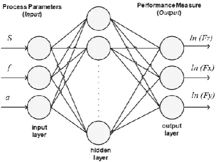
Within the frame of the present modelling work an ANN was developed in order to predict the three cutting force components (Fz, Fx, Fy) during longitudinal turning of AISI D6 tool steel. The three main cutting variables (S, f, a) were used as input parameters of the ANN model; see Fig.2.

The 27 experimental data samples (Table III), were separated into three groups, namely the training, the validation and the testing samples. Training samples are presented to the network during training and the network is adjusted according to its error. Validation samples are used to measure network generalization and to halt training when generalization stops improving. Testing samples have no effect on training and so provide an independent measure of network performance during and after training (confirmation runs); see [7, 13-15].

In general, a standard procedure for calculating the proper number of hidden layers and neurons does not exist. For complicated systems the theorem of Kolmogorov or the Widrow rule can be used for calculating the number of

hidden neurons [9]. In this work, the feed-forward with back-propagation learning (FFBP) architecture has been selected to model the cutting forces. These types of networks have an input layer of X inputs, one or more hidden layers with several neurons and an output layer of Y outputs. In the selected ANN, the transfer function of the hidden layer is the hyperbolic tangent sigmoid, while for the output layer a linear transfer function was used. The input vector consists of the three process parameters of Table III. The output layer consists of the performance measures, namely the Fz, Fx, and Fy cutting forces. Natural logarithm had been

performed on output data in order to improve the modeling procedure [19]; see also Fig. 2. Note, also, that cutting speed was divided by 100 for the same reason.

According to ANN theory, FFBP-NNs with one hidden layer are the most appropriate to model mapping between process parameters and performance measures in engineering problems [16].

In the present work, five trials using FFBP-NNs with one hidden layer were tested having 5, 6, 7, 8, and 9 neurons each; see Fig. 2. This one that has seven neurons on the hidden layer gave the best performance as indicated from the results tabulated in Table IV.

The one-hidden-layer seven-neurons FFBB-NN was trained using the Levenberg-Marquardt algorithm (TRAINLM) and mean square error (MSE) used as objective function. The data used were randomly divided into three subsets, namely the training, the validation and the testing samples.

Back-propagation ANNs are prone to the overtraining

TABLEIV

BEST PERFORMANCE OF ANN ARCHITECTURE. ANN Architecture

3x5x3 3x6x3 3x7x3 3x8x3 3x9x3 Training 0.996 0.997 0.998 0.999 0.999 Validation 0.828 0.929 0.978 0.855 0.498 Test 0.936 0.936 0.912 0.969 0.746 All 0.941 0.968 0.974 0.954 0.771 Best val. perf. 0.207 0.049 0.024 0.092 0.411 epoch 21 6 10 5 4

Fig. 3. Performance and training state. Fig. 2. The selected ANN architecture (feed-forward with

back-propagation learning).

problem that could limit their generalization capability [17]. Overtraining usually occurs in ANNs with many degrees of freedom [18]; after a number of learning loops, in which the performance of the training data set increases, while the performance of the validation data set decreases.

Mean Squared Error (MSE) is the average squared difference between network output values and target values. Lower values are better. Zero means no error. The best validation performance is equal to 0.0244 at epoch 10; see Fig. 3.

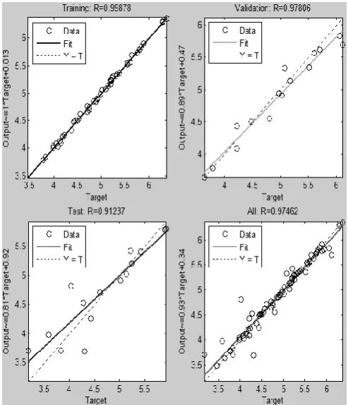
Another performance measure for the network efficiency is the regression (R); see Fig. 4. Regression values measure the correlation between output values and targets. The acquired results show a good correlation between output values and targets during training (R=0.998), validation (R=0.978) and testing procedure (R=0.912).

The mathematical relation of the input parameters to the output parameter is presented in the following formula:

    

  

    

 

  





 

S i

X j

i j j i

i sig w x b b

w

1 1

, 1 2

1 tan

2 purelin =

y (1)

where:

y: is the output value.

S: is the number of hidden neurons. X: is the number of inputs.

w1: is the vector of weights between the input and the hidden layer. The size of w1 is SX and w1i,j is the weight of the i neuron for the j input.

w2: is the vector of weights from the hidden layer to the output. The size of w2 is S1 and w2i is the weight of the i neuron to the output value.

b1: is the vector of biases of the neurons in the hidden layer. The size of b1 is S1 and b1i is the bias of the i neuron.

b2: is the bias of the output neuron.

purelin: is the linear transfer function and purelin(x) = x tansig: is the hyperbolic tangent sigmoid function and tansig(x) =





1 2

2 

 x

e

The weights and biases of Eq. 1 were calculated during the learning phase of the ANN, using the experimental data available (Table III).

The trained ANN model can be used for the optimization of the cutting parameters during longitudinal turning of an AISI D6 tool steel. This can be done by testing the behavior of the response variables (three cutting force components) when varying the values of cutting speed (S), feed rate (f), and depth of cut (a).

Fig. 5. Surface response of cutting force Fy for depth of cut, a= (0.5, 1; 1.5) mm and Kr=55o.

An example is presented in Fig. 5 where the surface response of cutting force Fy is plotted in relation with cutting speed and feed rate for three different values of depth of cut, a (0.5, 1, and 1.5 mm). It can be concluded that when the feed rate or the depth of cut is increased, the Fy is increased, too. It can be also concluded that the increase of the cutting speed affects the least, the cutting force Fy. These results are in accordance with the theory of metal cutting [2].

V. NEURAL NETWORK’S IMPLEMENTATION

A FFBP-NN model was built to estimate the three cutting forces (Fz, Fx, and Fy) response according to the cutting speed (S), feed rate (f), and depth of cut (a) during the longitudinal turning of AISI D6 tool steel specimens.

The performance of the network was found to be efficient providing very good correlation between outputs and targets during training (R=0.999), validation (R=0.953) and testing procedure (R=0.914).

Multi-parameter investigation of the process according to other quality indicators will be studied and analyzed in a future work.

VI. CONCLUSIONS

Cutting force calculation and modeling are major concerns in metal cutting theory. The accurate determination of cutting forces is essential for process performance and for developing machinability criteria. For the modeling of the cutting forces in longitudinal turning of AISI D6 tool steel grade various artificial neural networks were developed and tested. The suggested neural networks were trained with experimental data acquired from actual experiments with the neural network toolbox of Matlab®. The best performance was obtained from the ANN with FFBP architecture, one hidden layer and seven neurons on the hidden layer.

The results obtained indicate that the proposed modeling approach could be effectively used to predict the three component cutting force system during turning of AISI D6 tool steel, thus supporting decision making during process planning and providing a possible way to avoid time- and money-consuming experiments.

ACKNOWLEDGMENTS

The authors are grateful to Dipl.-Ing. J. Sideris, Director of Uddelholm Greece s.a. for the supply of the test material. They also wish to thank Mr. N. Melissas, technician at NTUA for performing the cutting experiments and Dipl.-Ing. P. Kostazos, Assistant at NTUA for helping with the cutting forces measurements.

REFERENCES

[1] N.M. Vaxevanidis, N. Galanis, G.P. Petropoulos, N. Karalis, P. Vasilakakos and J. Sideris,. “Surface Roughness Analysis in High Speed-Dry Turning of Tool Steel”, in Proceedings of ESDA2010: 10th Biennial ASME Conference on Engineering Systems Design and Analysis, July 12-14, Istanbul, Turkey, 2010 (paper ESDA2010-24811)

[2] G. Boothroyd and W. Knight, “Fundamentals of Machining and Machine Tools”, CRC Press, 2005.

[3] T. Szecsi, “Cutting force modeling using artificial neural networks”,

Journal of Materials Processing Technology, vol. 92-93, pp. 344-349, 1999.

[4] G. Dini, “Literature database on applications of artificial intelligence methods in manufacturing engineering”, Annals of the CIRP, vol. 46, no. 2, pp. 681-690, 1997.

[5] T.M.A. Maksoud, M.R. Atia and M.M. Koura, “Applications of artificial intelligence to grinding operations via neural networks”, Machining Science and Technology, vol.7, no. 3, pp. 361-387, 2003.

[6] E.O. Ezugwu, D.A. Fadare, J. Bonney, R.B. Da Silva and W.F. Sales, “Modelling the correlation between cutting and process parameters in high-speed machining of Inconel 718 alloy using an artificial neural network”, International Journal of Machine Tools & Manufacture, vol. 45, pp.1375-1385, 2005.

[7] A. Markopoulos, N.M Vaxevanidis, G. Petropoulos and D.E. Manolakos, “Artificial neural networks modeling of surface finish in electro-discharge machining of tool steels”, in Proceedings of ESDA2006: 8th Biennial ASME Conference on Engineering Systems Design and Analysis, July 4-7, Torino; Italy, 2006. (paper ESDA2006-95609).

[8] J. Kechagias, M. Pappas, S. Karagiannis, G. Petropoulos, V. Iakovakis and S. Maropoulos, “An ANN approach on the optimization of the cutting parameters during CNC plasma-arc cutting”, in Proceedings of ESDA2010: 10th Biennial ASME Conference on Engineering Systems Design and Analysis, July 12-14, Istanbul, Turkey. (paper ESDA2010-24225)

[9] S. Haykin, Neural networks, a comprehensive foundation, Prentice Hall, 1999.

[10] M.S. Phadke, Quality Engineering using Robust Design, Prentice Hall, 1989.

[11] J.P. Davim and L. Figueira, “Machinability evaluation in hard turning of cold work tool steel (D2) with ceramic tools using statistical techniques”, Materials and Design, vol. 28, no. 4, pp. 1186-1191 2007.

[12] H. Demuth and M. Beale, Neural networks toolbox for use with Matlab - User's guide, The MathWorks Inc, 2001.

[13] M. Pappas, J. Kechagias, V. Iakovakis and S. Maropoulos, “Surface roughness modelling and optimization in CNC end milling using Taguchi design and Neural Networks”, in ICAART 2011 – Proceedings of the 3rd International Conference on Agents and Artificial Intelligence, vol.1, pp. 595-598, 2011.

[14] M. Pappas I. Ntziantzias, J. Kechagias and N. Vaxevanidis, “Modeling of Abrasive Water Jet Machining using Taguchi Method and Artificial Neural Networks”, in NCTA 2011-International Conference on Neural Computation Theory and Applications, Paris, pp. 377-380.

[15] J. Kechagias and V. Iakovakis, “A neural network solution for LOM process performance”, International Journal of Advanced Manufacturing Technology, vol.43, no.11, pp. 1214-1222, 2009. [16] C.T. Lin and G.C.S. Lee, Neural fuzzy systems - a neuro-fuzzy

synergism to intelligent systems, Prentice Hall PTR, p 205, 1996. [17] S.G Tzafestas et al., “On the overtraining phenomenon of

backpropagation NNs”, Mathematics and Computers in Simulation,

vol. 40, pp. 507-521, 1996.

[18] L. Prechelt, “Automatic early stopping using cross validation: quantifying the criteria”, Neural Networks, vol. 11, no. 4, pp. 761-767, 1998.

[19] A.R. Alao and M. Konneh, “A response surface methodology based approach to machining processes: modelling and quality of the models”, Int. J. Experimental Design and Process Optimisation, vol. 1, no. 2/3, pp. 240-261(2009).