Polarization singularities in paraxial vector fields: morphology and statistics

Polarization singularities in paraxial vector fields:

morphology and statistics

M.R. Dennis

H.H. Wills Physics Laboratory, Tyndall Avenue, Bristol BS8 1TL, UK

Received 14 June 2002; received in revised form 3 September 2002; accepted 14 October 2002

Abstract

Polarization patterns in the transverse plane generically contain singularities: points of circular polarization (C points), lines of linear polarization (L lines), instantaneous zeros (disclinations) and component zeros. We investigate the geometry of ellipse fields at these singularities, using the Stokes parameters and others to characterize the singular geometry and morphology. Comparison is made with analogous structures on random surfaces, namely umbilic points and parabolic lines. The densities and correlations of the different types of polarization singularities are calculated in random polarization fields, and compared to the statistics of phase singularities and random surfaces.

2002 Elsevier Science B.V. All rights reserved..

PACS:42.25.Ja; 03.65.Vf; 02.50; 42.30.Ms

Keywords:Polarization; C points; Phase singularities; Stokes parameters; Gaussian randomness

1. Introduction

Polarization patterns in paraxial optical fields are geometrically complicated: the electric field vector at each point is moving, and for mono-chromatic fields, sweeps out an ellipse. The shape, size and orientation of the ellipse varies with po-sition in the transverse plane, and the most obvi-ous features of the overall pattern arepolarization singularities: places (usually points) where the el-lipse is circular (C points), curves along which the polarization is linear (L lines, or s lines), and points where the instantaneous vector vanishes (disclinations). These objects were appreciated as generic features of paraxial polarization fields by

Nye [1–3], and have been the subject of much subsequent research, in theoretical, numerical and experimental aspects [4–16]. They are the vector analog of phase singularities (zeros, wave disloca-tions, optical vortices) in scalar fields [17–19]; the geometry and topology of vector fields is richer, and so are the singular structures.

The purpose of the present paper is twofold. Firstly, to present the mathematics of polarization singularities in order to make their connection with phase singularities clear, and to emphasize the connections between the different kinds of singu-larities. Secondly, to present the calculations of polarization singularity densities in random isotropic paraxial vector wavefields, thereby www.elsevier.com/locate/optcom

complementing the corresponding description and statistics of phase singularities [19–24] and polar-ization singularities in nonparaxial three-dimen-sional fields [7]. The random wave model is a useful means to examine some of the properties of singularities Ôin the wildÕ, that is, thegeneric fea-tures of the singularities. The singular strucfea-tures arise naturally out of interference patterns, and are not due to any special symmetries. Attention will be restricted to monochromatic fields, and to the two-dimensional spatial structure in the transverse plane alone.

In addition to paraxial polarization patterns, two-dimensional fields of ellipses are found in the curvature fields on surfaces. That is, if fis a real, smooth function in the x;y plane, the gaussian curvature at a point in the plane is geometrically related to an ellipse. Places (generically points) where the curvature ellipse is circular are called umbilic points [25,26], and places (generically lines) where the gaussian curvature is zero (the curvature ellipse is linear) is linear are called par-abolic lines [26]; these places are important for focusing when the surface represents the surface of a lens, mirror or screen, and they organize the caustics arising from geometrical optics [3]. Geo-metric properties of random surfaces were previ-ously studied [25,27–29] mainly for this reason. In a sense, the present research applies these studies of geometric randomness to a different physical level: previous studies were on the geometric properties of surfaces as lenses, and their aim was to characterize the focusing of rays from them; the present work aims to do this for the morphology of the polarization wave patterns themselves. However, the calculations bear strong similarities to their random surface counterparts, as will be discussed.

Fields of ellipses also occur in oceanography, since the (changing) tidal current vector sweeps out an ellipse in time, so the ocean tidal current may be represented by a two-dimensional field of phased ellipses (for instance, see the figures of [30]), which generically has C points, L lines, and disclination points. The locations and nature of the C points in the North Sea were discussed in [8]. The morphology described in the present work applies to tidal singularities, although the

statis-tics, which rely on an isotropic linear random wave model, do not. There are also similarities to the general flow fields studied in [31]. Geometrically close to C points are line field singularities, which occur physically as defects in plane confined liquid crystals [32], morphological features of fingerprint patterns [33], and in partial polarization patterns arising from scattering in the atmosphere from astronomical sources [34], and from sunlight [35,36].

The most important tool in the study of any type of wave pattern singularity are phase singu-larities, that is, the zeros of a complex scalar field

w¼wðx;yÞ ¼wðRÞ(we only consider fields in two dimensions). Ifwrepresents an optical scalar field, the phase singularities are wave dislocations (op-tical vortices). Writing w¼nþig¼qexpðivÞ (whereqP0,v;n;gare real), the phase singulari-ties are places where the real and imaginary zero contours cross, and at these places the amplitudeq

vanishes and the phasev is indeterminate (singu-lar). Phase singularities generically occur at points, and all equiphase lines (lines of constantv) meet at them. Around the singularity, the phase must change by 2ps, where s is an integer, positive, negative or zero.sis called thedislocation strength

(or topological charge) of the singularity; the

strength is positive if the phase increases in an anticlockwise sense, and decreases otherwise. Therefore, around a closed curve L which does not cross a zero ofw, the line integral

I

L

dv¼ I

dR rv¼2ps ð1Þ

gives the total dislocation strength enclosed byL. Generically, phase singularities have strength 1, but more than one singularity may be enclosed by

L. For strength 1 singularities, the sign of s is given by the sign of the functionD[19,20],

D¼nxgygxny: ð2Þ

The foregoing discussion does not requirewto be a wavefield itself.

of describing C points and their structure are gi-ven, realized as phase singularities of different scalar fields. Section 4 follows with a description of L lines and relative singularities (component zeros, disclinations) found on them. The statistical den-sities of C points and L lines are computed in Appendix B, using the isotropic random wave model formulated in Appendix A; the results are quoted and described in Section 5.

The main results of this paper are:

• The introduction of the phase sphere and asso-ciated phase parameters (Eq. (18)) as a descrip-tor of polarization ellipses complementary to the Poincaree sphere and Stokes parameters.

• The expressionsDL;DC(Eqs. (29) and (30)),

giv-ing the line and contour classification types of C point in terms of Stokes parameters.

• Example (31), generalizing the C point example of [8] to include all possible morphologies of C points (including the contour classification).

• Expression (40), which proves the main result of [15] in a simple way.

• The statistical results of Section 5, which gives the density (Eq. (41)) and correlation functions (Eqs. (46) and (47)) of C points in isotropic ran-dom fields, related to the corresponding disloca-tion statistics described in [19]. The Venn diagram of different fractions of types of C point is derived (Fig. 9), and compared to the corresponding diagram for umbilic points de-rived in [25]. The density of L lines is also given (Eq. (54)), and their statistical geometry and percolation properties are briefly compared to the curvature properties of random surfaces.

2. Polarization ellipse morphology

This section is concerned with the mathematical formalism of paraxial polarization, including the Stokes parameters and Poincaree sphere. Much of this description, with the exception of the phase sphere at the end of the section, can be found in standard textbooks, such as [37]. We are interested in the geometric structure of a two-dimensional complex vector wavefield E¼Eðx;yÞ ¼EðRÞ, representing the electric field in the transversex;y

plane of a paraxial wavefield (i.e., E is the Jones

vector at R). E may be rewritten in terms of cartesian components, or real and imaginary parts:

E¼ ðEx;EyÞ ¼pþiq: ð3Þ

The physical quantities E;p;q (and others) are taken to be smooth functions of position, although for brevity R dependence is usually not written explicitly. Derivatives will be represented by sub-scripts after scalars (as in Eq. (2)), and by commas after vector components (e.g., olEk¼Ek;l). The

modulus of a real vector is denoted by italics, for instancejVj ¼V.

The wave is monochromatic, and its time de-pendence is given by a phase factor expðixtÞ;

where x is the unique angular frequency associ-ated with the field. The real physical disturbance is

ERe_v ¼ReEexpðivÞ ¼pcosvþqsinv; ð4Þ where v¼xt. Instead of explicitly treating time dependence of the field, E is dependent on the abstract phasev. Elementary linear algebra shows thatERe_v sweeps out an ellipse from its centre, asv

increases. The orthogonal semiaxes of the ellipse are denoted by p₀;q₀, with p0Pq0. If ERev rotates

anticlockwise as v increases then E is said to be right-handed(RH), if clockwise, left-handed(LH). If E is RH, the two-dimensional cross product ImEE¼2pq is positive, and if LH, it is negative.

The cartesian components Ex;Ey are complex

scalar fields. Using a circular basis, E may be re-written

E¼wReRþwLeL; ð5Þ

where w_R;w_L are the right- and left-handed cir-cular components of E, and the circular basis vectors, in cartesian coordinates, are defined

eR¼

1 ffiffiffi 2

p 1

i ; eL¼ 1

ffiffiffi 2

p 1

i

: ð6Þ

The phases of w_R;w_L are defined asvR;vL

respec-tively. With these definitions, the right-handed component circulates in the anticlockwise direc-tion. Note that some authors with this convention define the right-handed circular unit vector aseR:

therefore a special phasev0such that the real and

imaginary parts of the resulting vectorEexpðiv0Þ

are perpendicular, in the direction of the semiaxes

p₀þiq0¼Eexpðiv0Þ

¼ ðpcosv0þqsinv0Þ

þiðqcosv0psinv0Þ: ð7Þ

Since the real and imaginary parts of (7) are or-thogonal, it is possible to show that

v0¼

1 2 arctan

2pq

p2_q2¼

vRþvL

2

¼1

2 argwRwL; ð8Þ

which is only defined modulo p. This phase was denoted by ein [37] and [1]. Nye [1] called v0 the Ôphase of the vibrationÕ, but we use the more concise term rectifying phase, because it rectifies (makes right-angled) the real and imaginary parts p;q.

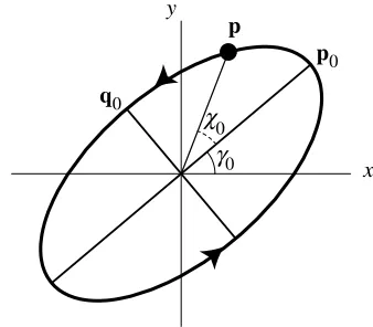
Geometrically, the orientation of the ellipse is specified by the angle c0 between the major

semi-axisp₀ and thex-axis

c0¼arctan p0y p0x

: ð9Þ

Using Eqs. (7) and (8), this may be written solely in terms of the components of p;q, where, after simplification

c0¼

1 2 arctan

2ðpxpyþqxqyÞ p2

xþq2xpy2q2y

¼vLvR 2

¼1 2 argw

RwL: ð10Þ

This expression is similar to expression (8) for v₀, and is also only defined modulo p. The relation between the geometry of the polarization ellipse and the parameters defined here are shown in Fig. 1.

The polarization matrix (coherence matrix, or

Stokes matrix) MS is a 22 hermitian matrix

defined by its components

MSkl¼EkEl; k;l¼x;y; ð11Þ

and its real partMReMS is a positive definite symmetric matrix whose eigenvectors are in the directionsp₀;q₀, and whose eigenvalues arep2

0and q2

0. In fact, M

1

, if it exists, is the quadratic form

matrix for the ellipse. The four components of the complex polarization matrix with respect to the usual Pauli spin matrices are known as theStokes parametersS0;S1;S2;S3, i.e.,

MS ¼1 2

S0þS1 S2iS3

S2þiS3 S0S1

; ð12Þ

and they are given by

S0¼ jwRj 2

þ jwLj 2

¼ jExj 2

þ jEyj 2

¼p2 xþp

2 yþq

2 xþq

2 y; S1¼2 Reðw_Rw_LÞ ¼ jExj

2

jEyj 2

¼p_x2þq2_xp2_yq2_y;

S2¼2 Imðw_Rw_LÞ ¼2 ReðE_xEyÞ

¼2ðpxpyþqxqyÞ;

S3¼ jw_Rj2 jw_Lj2¼2 ImðE_xEyÞ

¼2ðpxqypyqxÞ:

ð13Þ

The expressions for Si (i¼1;2;3) in the circular

components w_R;w_L are evidently a cyclic permu-tation of the expressions in cartesian components

Ex;Ey; this is because the Pauli matrices (which

give the Stokes parameters) are permuted by the transformation between the cartesian and circular basis (6), as may be easily checked. Physically, S0

represents the intensity jEj2 of the field, and

pjS3j=2 is the area of the polarization ellipse; the

sign ofS3gives the handedness of the ellipse, + for

RH,) for LH (it is equal to pq). By (10) and (13), tan 2c0¼S2=S1. The Stokes parameters are

independent of the rectifying phasev0.

The Stokes parameters, as defined, satisfy

S₀2¼S₁2þS₂2þS₃2; ð14Þ

confirming that the polarization is pure, and they can be normalized

si¼Si=S0; i¼1;2;3: ð15Þ

The unit vector (s1;s2;s3) is called the (normalized)

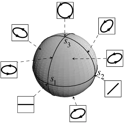
Stokes vector, and its direction in abstract Stokes space describe the orientation and shape of the polarization ellipse. The possible states of polari-zation are therefore parameterized by positions on the unit sphere, called the Poincaree sphere. All possible polarization ellipses (up to size, given by

S0, and rectifying phasev0), are parameterized by

position on the Poincaree sphere, given by the spherical polar angles a;b. The geometry of the Poincaree sphere is shown in Fig. 2. The orientation

c0 is governed by the azimuthal angle

b¼2c0; ð16Þ

and the polar anglea¼arccoss3 is related to the

eccentricityeof the ellipse, whose square is found to be given by the following expressions:

e2_¼1q 2 0 p2 0

¼ 4jwRjjwLj ðjwRj þ jwLjÞ

2

¼ 4 tana=2 ð1þtana=2Þ2

¼ 2

S2 3

S0

ffiffiffiffiffiffiffiffiffiffiffiffiffiffiffiS2 0S23

q ffiffiffiffiffiffiffiffiffiffiffiffiffiffiffi

S2 0S32

q

: ð17Þ

The eccentricity therefore changes with latitude: at the poles, it is 0(circular polarization), gradually increasing to 1 (linear polarization) on the equa-tor. RH polarization is in the northern hemisphere (S3>0), LH in the southern (S3<0). The axis

ratio, signed by handedness, is given by tanðp=4a=2Þ.

The information about the rectifying phasev0is

lost in the Stokes parameters (13), which only contain information about intensity, handedness, eccentricity and orientation (which are measurable quantities). It is therefore possible to define a sphere equivalent to the Poincaree sphere, but using the rectifying phase v0 rather than orientation

anglec0as azimuth [38]. The cartesian coordinates

on the phase sphere are given by the phase pa-rameters (cf. Eq. (13))

T0¼ jEj2¼S0;

T1¼2 ReðwRwLÞ ¼p 2_q2_; T2¼2 ImðwRwLÞ ¼2ðpqÞ; T3¼ jwRj

2

jwLj 2

¼S3:

ð18Þ

The zeroth and third phase parameters are iden-tical to the corresponding Stokes parameters, so the eccentricity dependence on latitude (17) is the same as on the Poincaree sphere.T1andT2 are the

same as the corresponding Stokes parameters ex-cept wR is no longer conjugated, equivalent to

exchangingpy andqx. The azimuth arctanT2=T1is

equal to 2v0, from (8). Therefore, the phase

(vi-sualized as the position ofp¼ReEon the ellipse), varies with azimuth around the sphere.

It is worth noting that the geometry described above only applies to ellipse fields in two dimen-sions, when the ellipses are all confined to the plane. If the polarization field is nonparaxial, and the plane of the ellipse changes from point to point, the Poincaree sphere is no longer appropriate to describe the state, since the ellipse has no unique Fig. 2. Depiction of the Poincaree sphere, with cartesian axes

handedness. The correct polarization geometry can be found using the Majorana sphere [39,40], and this leads to some differences in the geometry of polarization singularities in paraxial and non-paraxial fields [4,7,8].

3. C points and their geometry

The most important type of polarization sin-gularities are C points [1], that is, places in the polarization field where the polarization is circular (either RH or LH). This generically happens at points because C singularities have codimension 2, that is, two real conditions on the field variables must be satisfied for the polarization to be circular. They may be viewed in several different ways:

• The real and imaginary vectorsp;qare of equal length and orthogonal. This pair of conditions holds for both the paraxial and nonparaxial case, and has been used as the definition of C points several times in the literature [1,3,8,11]. Note that this geometric condition is equivalent to the requirement on the phase parameters

T1¼p2q2¼0ðequal lengthÞ

T2¼2pq¼0 ðorthogonalÞ

at a C point:

ð19Þ

The vanishing of these two parameters is equivalent to the statement that the rectifying phase v0 is undefined (singular) at a C point,

sincep;q are rectified for any phase.

• The Stokes parameters S1;S2 vanish at the C

point. The two points of circular polarization on the Poincaree sphere lie at the north and south poles, where S3¼ S0, and so S1¼S2¼0by (14). The azimuthal angle b is singular at the poles of a sphere, and this corre-sponds to the singularity of the orientation an-glec0: no unique semiaxes can be defined for a

circle. This is a different singularity from that of

v0, although the two singularities always occur

together, at the poles of the phase sphere and Poincaree sphere. The C point is RH ifS3¼S0,

LH ifS3¼ S0.

• The real symmetric matrixMis degenerate (this is obvious from the above point and the

defini-tion (12)). Degeneracies of real symmetric ma-trices are studied in more general contexts [41,42], and all have codimension 2. The struc-ture of these matrices around the singularity is called adiabolical pointbecause the two eigen-values locally have a double cone structure. This interpretation was used to define the umbi-lic points of a real function f in [25,3], as degeneracies of its hessian matrix H¼fab

(a;b¼x;y).

• The simplest and possibly most instructive way of viewing C points is to consider the circular components w_R;w_L; a point of RH circular polarization occurs wherew_L ¼0, and equiva-lently LH circular polarization wherew_R ¼0 – that is, C points are dislocations of wR;wL

[1,3,5]. The phasesvR;vL are therefore singular

at the respective C points, and by Eqs. (8), (10),

v0 andc0are automatically both singular when

eithervR orvL is.

The above implies that the ellipse orientationc0is

undefined at a C point. As with phase singularities and vector fields, this implies that the line integral on a loopL,

1 2p

I

L

dR rc0¼I; ð20Þ

is quantized as in (1), but in units of 1/2 sincec₀is only defined modulop. This numberIis said to be the C point index, and is generically 1=2. C points may be thought of as singularities in line fields (that is, fields ofÔheadless vectorsÕ[32]); lines are brought back to themselves after half a full rotation, and this happens generically around a C point.

So far, we have seen that generic C points may be classified into four types, according to hand-edness (RH or LH) and index (1=2). A scalar field may be defined from the Stokes parameters [9–11]

r¼S1þiS2: ð21Þ

This vanishes exactly at a C point (where

S1¼S2¼0), and its phase is clearly

argr¼b¼2c0: ð22Þ

sign of the index of a C point can therefore be found as signDI, whereDIis defined

DI¼S1xS2yS1yS2x; ð23Þ

theranalog to Eq. (2). This agrees with the form stated in Appendix 3 of [31].

C points are also phase singularities in the cir-cular componentsw_L;w_R, but how do the signs of these dislocations agree with the C point index? By Eq. (13),

r¼w_RwL; ð24Þ

implying that the strength of the dislocation inwL,

at a RH C point, has the same sign as the C point index there, but the strength of a dislocation ofw_R, at a LH C point, is minus the sign of the C point index (this may also be seen using (10) [5]). r is therefore a complex scalar field which has phase singularities exactly at the C points, and the signs of its phase singularities are the same as the C point indices. However, just like the Stokes pa-rameters themselves, this field is not itself a solu-tion of any wave equasolu-tion, and is quadratic in the field variables.

An alternative scalar with nodes at C points was used by [7,8], and is defined as the scalar product ofEwith itself

u¼EE: ð25Þ

This vanishes when the polarization is circular, and from Eqs. (18),

u¼T1þiT2¼wRwL: ð26Þ

Its phase argu is clearly equal to 2v0, and the

modulijuj;jrjare equal

juj2¼ jrj2¼S2₀S2₃¼ ðp2₀q2₀Þ2¼p₀4e4: ð27Þ Eq. (26) shows that the sign of a phase singularity inuis always the same as the dislocation strength in the circular component at that point, and therefore is opposite in sign to the C point index at a LHC point. The equiphase lines ofuare lines of constant v0; the lines T1¼0and T2¼0, from

(18), are respectively lines along which p and q have equal length, and are orthogonal. The equi-phase lines of r are lines where the orientation angle uis constant, the a-lines discussed by [16]; we suggest the more evocative name isoclines for these lines. As complex scalar fields, r;u;wR;wL,

satisfy the myriad sign rules discussed by [22]. Each of these phase functions has saddles and possibly maxima and minima, which are station-ary points of the appropriate angle, as described by [16].

C points are singularities of their orientation angle c0, which represents an undirected line at

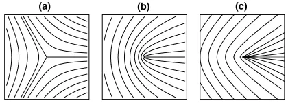
each point; we therefore discuss the wider but morphologically close phenomenon of line sin-gularities. Line fields can be classified according to their index, that is, the signed number of turns the line makes around the singularity in a right-handed sense, in units of 1/2. The number of straight lines that terminate on the singularity is generically 3 or 1. This is the line classification, and for index 1=2 singularities, it is always 3; such a singularity is called a star. If the index is þ1=2, it may either be 1 or 3, and the two morphologies are called lemon and monstar, re-spectively [25]. The three singularity types in line fields are shown in Fig. 3. The four polarization neutral points that occur from sunlight scattering in the atmosphere [35,36], not described by the present theory since they involve partial polari-zation, are nevertheless generic index +1/2 line field singularities, and the polarization pattern around them is of lemon type (as can be seen from the figures in [36]).

In Section 5 the relative densities of lemon, monstar and star types of C point in gaussian random polarization fields are discussed, comple-menting the corresponding calculation [25] for umbilic points. In fact, it was in the context of umbilic points that this classification was origi-nally recognized [25,26], where the linefields are the principal curvature directions (and so are

gular at degeneracies of the hessian, as previously observed).

In order to distinguish between the line classifi-cation types, we need a quantity equivalent toDIin Eq. (23) whose sign gives the type of line classifi-cation. The quantity defined in Eq. (6) of [25] is not appropriate for C points, because the derivatives of the components ofMare more general than those of H. However, the appropriate expression for C points may be derived as follows. The C point is translated to the origin, andS1;S2in the expression c0¼arctanðS2=S1Þ=2 are expanded to first order (at

the C point) with polar coordinatesR;h, with angle

h¼arctanðy=xÞ. This expression is rearranged to a polynomial equation int¼tanh,

S2yt3þ ðS2xþ2S1yÞt2þ ð2S1xS2yÞtS2x¼0;

ð28Þ

whose solutions give the angles whereh¼c0, that

is, the angles of the straight lines terminating at the singularity. The number of these solutions is given by the discriminant of the polynomial (28), which is (up to an unimportant numerical factor)

DL¼ ðð2S1yþS2xÞ 2

3S2yð2S1xS2yÞÞ

ðð2S1xS2yÞ 2

þ3S2xð2S1yþS2xÞÞ

ð2S1xS1yþS1xS2xS1yS2yþ4S2xS2yÞ 2

: ð29Þ

The sign of the discriminant gives the number of roots – 3 (star or monstar) ifDL>0, 1 (lemon) if DL<0. This expression is equivalent to that of

[31], and Eq. (6) of [25] after the appropriate substitution for umbilic points.

There is an additional classification, thecontour classificationwhich specifies whether the singular-ity is elliptic or hyperbolic, according to whether the contour lines of the eigenvalues of M around the degeneracy are ellipses or hyperbolas. For umbilic points, this classification determines whe-ther the resulting catastrophe of the normal rays is the elliptic or hyperbolic umbilic catastrophe [3]. It is not clear whether there is any correspondingly simple physical interpretation for this classification for C points. The function DC, whose sign

deter-mines the contour classification, was stated in [31] Appendix 3; in terms of Stokes parameters, it is proportional to

DC¼ ðS1xS2yS1yS2xÞ 2

ðS1xS0yS1yS0xÞ 2

ðS0xS2yS0yS2xÞ 2

: ð30Þ

The point is elliptic if DC>0, and hyperbolic if DC<0. It may be readily checked that, atR0,DC

is the gaussian curvature of the surface locally defined detðMðRÞ MðR0ÞÞ; this surface – whose

interpretation also holds for umbilic points – is the product of the differences of the two eigenvalues of

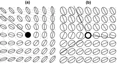
Mfrom their degenerate value. Two C points from a random polarization pattern are shown in Fig. 4, with their line and contour types indicated.

An instructive example is the field

Eex¼ð þ1 iðaxþbyÞ;ið1xÞÞ; ð31Þ

wherea;b are real. There is a RH C point at the origin, and its classification parametersDI;DL;DC

are

DI¼4bð1þaÞ; ð32Þ

DL¼ 16bð2þ2abÞ3; ð33Þ

DC¼64ab2: ð34Þ

The form witha¼0was given in [8] Eq. (17). All six morphological types are clearly possible (el-liptic or hyperbolic, lemon, star or monstar) with appropriate choices ofaandb, as shown in Fig. 5. The conjugate fieldE_exto (31) has a LH C point at the origin (the classification parameters in (34) are

unchanged), so all 12 types of C point are realiz-able from this example. Bothaandbare required to realize all of the types, so the Venn diagram of different morphological types, shown in Fig. 5, is two-dimensional, unlike the umbilic point case where it is only one-dimensional [25].

The number of C points in a given areaAof the plane, #C;A is

#C;A¼

Z

A

d2RdðS1ÞdðS2ÞjDIj: ð35Þ

The d-functions pick out the C points only, and the modulus ofDIgives the correct jacobian for an

integral in real space. It is analogous to the ex-pressions given in [19,20] for phase singularity densities; this is the equivalent form for phase singularities inr. Eq. (35) gives the same result if

S1;S2are replaced byT1;T2. The density of lemon, monstar, star, elliptic, hyperbolic, LH, RH types (or a mixture) in A can be calculated by multi-plying the integrand in Eq. (35) by the appropriate product of step functions HðDLÞ;HðDIÞ;HðS3Þ, etc.

If the polarization field is nonparaxial, the po-larization is circular along lines, called CT lines (or C lines) [4,7], which cross an (arbitrary) plane at points. The scalaru¼EE, which is defined when the field is nonparaxial, has phase singularities

along CT lines. The scalarris not defined in these fields, because the Stokes parameters are not well-defined.

4. L lines and relative singularities

The second type of singularity we consider are places where the polarization is linear, that is, when the third Stokes parameterS3¼0. vanishes.

The locus where this happens is therefore codi-mension 1, giving lines in the transverse plane – they were introduced by Nye [2], who called them s lines. Following more recent work [8,16], we call them L lines. On L lines, the handedness of the ellipse is not defined (singular), consistent with the fact that the singularities of fields specified by a discrete parameter (i.e., signS3) have codimension

1; in this case, the L lines separate regions of RH and LH polarization.

The vanishing ofS3¼T3 can be interpreted by Eq. (13), as the vanishing of the cross product ofp andq, that is, the vectors are (anti)parallel, and the complex vector E becomes a real vector times a complex phase factor. Both the plane angle of this real vector (equivalent toc0) and its complex phase

(equivalent to v0), change continuously along the

L line. In terms of circular components, Eq. (13) implies that jwRj ¼ jwLj on an L line, and the

phasesvR;vL change continuously along it. Unlike

C points, which have a rich topological structure, there is no characteristic structure around an L line; generically,S3passes through zero smoothly,

and the angles c₀, v₀ change smoothly along the singular line. The analog of L lines for surfaces is where the gaussian curvature, defined as the hes-sian determinant HdetH¼0. These are the parabolic lines [26], separating regions of positive curvature from negative curvature. Their signifi-cance in focusing was described by Berry [43], who showed that caustic lines in the far field are de-formed images of the parabolic lines on the fo-cusing surface.

The vectorUL, defined to point in the direction

of an L line with the RH region on the left, is easily defined: since rS3 points into the RH region, it is

UL¼ ðS3y;S3xÞ: ð36Þ

Note that, with this definition, jULj ¼ jrS3j. The

length of L line in an areaAof the plane is given by the integral

‘L;A¼

Z

A

d2RdðS3ÞjrS3j; ð37Þ

and the number of L line crossings on a specified lineLin the plane is given by

#L;L ¼

Z

L

dRdðS3ÞjS30j; ð38Þ

where the integral is along L, and S0

3 is the

deriv-ative ofS3 along this line.

There are two further types of singularity, found on L lines, which we call relative singulari-ties, because their singular nature is relative to a chosen phase or orientation. The first are the zeros of the instantaneous real field ERe_v ; these are ge-nerically points, which may have a source, sink, circulation, spiral or saddle morphology, and are calledwave disclinations[2]. They can only exist on L lines, because otherwise ERe

v is never zero.

Throughout an entire cycle, 06_v6_{2p, each point}

on the L line is a disclination twice, and the dis-clination points move along the L line as v in-creases. Disclinations are relative singularities, since their position is phase-dependent, unlike C points and L lines, whose position is independent of phase. Thedisclination indexis defined to be the Poincaree index of the zero of the real field ERe_v , which may be shown to be the sign of the function

Ddisc, (cf. Eqs. (1), (2) and (20))

Ddisc¼ERevx;xE Re vy;yE

Re vx;yE

Re

vy;x: ð39Þ

On an L line, the minor semiaxis q₀ is zero, and E¼p₀expðiv₀Þ from (7), implying that ERe_v ¼ p₀cosðv₀vÞ, which is zero (a disclination) when

v0v¼p=2 mod p. Disclinations for different v

can therefore be identified by the crossings of the phase contours of u with L lines. On the phase sphere, they correspond to particular points (given by the phasev) on the equator.

The analog of disclinations on the Poincaree sphere are component zeros or component vortices [13–15]: if a point of linear polarization on an L line has orientation angle c0, the component ofE

in the direction c0þp=2 is zero (a phase

singu-larity). These singularities, relative to a choice of

c0, are readily measurable using polarizers. Hajnal

[5] section 6 derived a topological result, relating the number of disclinations on a closed L loop with the total index of C points enclosed, namely that the sum of disclination indices on the L line is equal to2ptimes the C point index enclosed by the L loop. The analogous statement for compo-nent zeros was made by [14,15]. In the following, we prove this result more simply than in [15].

Consider a place on an L line (not necessarily closed) where Ey¼0; at this point, S1¼S0, S2¼S3¼0and through the point,c0is smoothly

changing. We will show that the sense of rotation of c0, along the L line in the direction of Us, is

equal to the dislocation strength (2) of the com-ponent zero. The rate of change ofc0 along the L

line is

Us

jUsj

rc0¼

ðS3y;S3xÞ

jUsj

ðS1S2xS2S1x;S1S2yS2S1yÞ

S2 1þS

2 2

¼ 1

S1jUsj

ðS2xS3yS2yS3xÞ

/signS1signðS2þiS3Þ

/py;xqy;ypy;yqy;x; ð40Þ

where Eqs. (10) and (36) have been used in the first line, S2¼0at the zero point in the second, and

S1>0 (Ey¼0) in the third. The result in the third

equality is the sign of the phase singularity inEy,

and this result generalizes for a zero in any com-ponent by rotating the plane. Note that the second line involves the sign of the topological charge of the Stokes field S2þiS3 [9]. Around a closed L

loop enclosing a RH region, the C point index enclosed, by Eqs. (20) and (40) equals the total topological charge of the component zeros on the L line, for any choice ofc0. If a LH region is

en-closed, the sign of Us must be reversed, so the C

point index enclosed is minus the sum of topo-logical charges of the component zeros. Similar results for disclinations hold, but v0 replaces c0

(and other quantities in the derivation are replaced from their Poincaree sphere to their phase sphere versions). An ellipse pattern around a closed L loop containing a C point is shown in Fig. 6.

1 as in the paraxial case). They are called LT _lines

(or L lines) [4,7], and are singularities of the di-rection of the normal to the polarization ellipse. The difference in codimension reflects the topo-logical difference between the Poincaree sphere and the Majorana sphere [11,40].

5. Polarization singularities in isotropic random fields

We now apply our study to polarization sin-gularitiesÔin the wildÕ, that is, in isotropic gaussian random complex vector fields. Since we are as-suming monochromaticity, for each realization of the random function, there is a well-defined ellipse at each point in the plane with a well-defined in-tensity, eccentricity and (possibly singular) orien-tation angle and rectifying phase. The scalar analogs of these fields have been studied as a model for speckle fields [44,45], and the scalar singularity behaviour by [11,19–22,24]. Other studies have calculated the statistics of geometric properties of the polarization ellipse [46,47] and Stokes parameter statistics [48–50], but not nec-essarily for fields (instead, the randomness is in time, which is not relevant here); by ergodicity of the gaussian model, spatial averages are equal to ensemble averages.

The fields are taken to be the sum of plane waves with random phases, equally distributed in

direction, and are described in Appendix A; the circular components wR;wL, and equivalently the

cartesian components Ex;Ey, are independent

identically distributed circular gaussian fields, whose derivatives are also independent gaussian random fields. The two-dimensional model is a generalization of that considered in [19], where more details may be found. The random field, as defined, is extremely democratic; for instance, the areas of LH and RH polarization are equal on average, and only generic singularities contribute to their averages. The details of the calculations may be found in Appendix B, and only the re-sults are discussed here. The random surface we will compare with is simply a real scalar com-ponent of this complex gaussian random field model; it is discussed in more detail in [25,27–29]. The pattern in one square wavelength of a ran-dom wave with the ring spectrum is shown in Fig. 7.

Fig. 6. The ellipse field near a closed L loop, enclosing a region of RH polarization (shaded). One C point, marked

Fig. 7. One square wavelength (ð2p=KdÞ 2

) of a random paraxial field with the ring spectrum, constructed by superposing 50 monochromatic random waves from Eq. (A.1). The RH regions are shaded, and separated from the LH regions by L lines (solid lines). C points are represented by

The density of C points in the paraxial planedC

is the ensemble average of the density expression (35), and is

dC¼

K2

2p¼0:15915K2; ð41Þ

whereK2denotes the second moment of the power

spectrum [19]. This result agrees with, and can simply be derived from, the fact that C points are dislocations in the circular componentswL;wR; the

density of dislocations dD in a random complex

scalar paraxial wavefield was calculated in [19–21] to be

dD¼

K2

4p: ð42Þ

The total C point density is the sum of dislocations in wR;wL, each of which contributes a density of dD, sodC¼2dD, and the densities of LH and RH

C points are equal. The mean C point index is also zero – a consequence of the global neutrality of dislocation strength, discussed in [21,23]. In Fig. 7, there are 9 C points: five lemons (two RH, three LH) and four stars (two RH, two LH). The ex-pected number, in one square wavelength of the ring spectrum (4p2_=K2

d), is 2p, slightly fewer than

in this sample. The total topological charge in this square is 1. The interpretation of C points as dis-locations means that many statistical results pre-viously derived for dislocations apply to C points; for instance, [20] computed the dislocation densi-ties in anisotropic fields and in a longitudinal plane, in addition to the paraxial plane; these re-sults apply directly to RH and LH C points.

In any realization of the random field (i.e., a sample function), the densities of C singularities at two separated points are not independent, but depends on their separation. In our isotropic model, the direction of separation is unimportant, and the average of two local C point densities (of possibly different types), at points separated by

R¼ jRj, is given by thecorrelation functions, nor-malized by the C point density. This implies that when the densities are independent (for instance, for large R), the correlation is 1. The theory of correlations for wave dislocations in the plane is studied by [19,21,23,51], using results and nota-tions from the statistical mechanics of fluids and plasmas [52]; the dislocation correlation functions

are themselves functions of the field autocorrela-tion funcautocorrela-tion CðRÞ, defined in Eq. (A.7). We will use the notation of [19], to which the reader is referred for details; for instance, the partial cor-relation function between types i;j is denoted by

gijðRÞ ¼gij, which equalsgji by isotropy.

Correlations are examined between four differ-ent types of C point-index: +1/2 RH, 1=2 RH, +1/2 LH,1=2 LH. Of these, all RH densities are independent of LH densities (since they are dislo-cations of the independent fieldswR;wL), so, in an

obvious notation

g_þRþL¼gþRL¼gRþL¼gRL¼gþLþR

¼gþLR¼gLþR¼gLR¼1: ð43Þ

The partial correlations between C points of the same handedness is clearly the same as the corre-sponding correlations for dislocations, denoted by

g_þþ¼g;g_þ¼g_þ, so

gþRþR¼gRR¼gþLþL¼gLL¼gþþ; ð44Þ

gþRR¼gþLL¼gRþR¼gLþL¼gþ: ð45Þ

The total number correlation functiong¼gðRÞis the sum of all the 16 partial correlations, divided by 16 in order thatgðRÞ !1 asR! 1,

g¼ 1

16 X

ij gij¼

1 2þ

1

4ðgþþþgþÞ

¼1 2þ

gD

2 ; ð46Þ

where i;j¼ þR;þL, etc. and gD represents the dislocation number correlation function [19].

It is also possible to calculate the C point charge correlation functiongI, that is the total correlation function with local densities weighted by their index (for dislocations, by topological charge). It is

gI¼

1 16

X

ij

signðijÞgij¼

1

4ðgþþgþÞ

¼gQ

2 ; ð47Þ

where gQ is the dislocation charge correlation

function [19,21]. The C point correlation functions

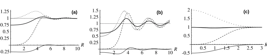
g, gI, gþþ, and gþ are shown in Fig. 8, for the

each other, satisfying the C point analog of the first Stillinger–Lovett sum rule [52]

dC

Z

d2RgIðRÞ ¼2pdC

Z 1

0

dR RgIðRÞ ¼ 1; ð48Þ

that is, each C point is surrounded by a cloud of C points of the opposite index. Note that screening only takes place between C points of the same handedness. These screening results are discussed further and compared with simulation data in [53]. The overall density of C points may be com-pared to the number of nonparaxial CT line crossings of a plane, which were calculated for isotropic fields in [7], Eq. (5.10). After changing to a correct plane projected spectrum [19], the density is

d_CT ¼

3K2

4 3 10p

þ 1 5pffiffiffi3

¼0:15822K2: ð49Þ

The numerical value is therefore very close to dC,

although no approximation has been made in ei-ther calculation and the analytic forms in (41) and (49) are rather different. Physically, there is a sig-nificant difference in the two fields – the circular polarization ellipses of the CT points do not lie in the plane in which the density is measured. This phenomenon, where two random quantities which are similar physically and give numerically close but analytically different values, also appears for the density of nonparaxial LT lines crossing a plane, given in [7], which is close numerically to

d_CT. It appears again in the comparison of densities of L lines and parabolic lines, described below.

The C point density may also be compared to the umbilic point density on isotropic random surfaces; the total umbilic point densitydUwas calculated in

[25] to be

dU¼ K6

4pK4

: ð50Þ

The factorK6=K4involves higher moments than the C point density, because umbilic points are singu-larities in higher derivatives of the field. Apart from this spectral factor, the density is half that of C points, or equal to the density of RH C points.

The fractional densities aC of the lemon, mon-star, star fractions of C points are calculated in Appendix B (for total density, multiply by dC)

aC;star¼0:5; aC;monstar¼0:05279; aC;lemon¼0:44721:

ð51Þ

These are precisely the same as the fractions for umbilic points, calculated in [25] Eq. (41). Since the star singularities are precisely those with index 1=2, aC;star must be 1=2 since the total charge

density is zero. Just over a 10th of the indexþ1=2 points are monstars, and the rest are lemons. The fractions are the same for RH and LH C points.

The density fractions for C points under the contour classification (E for elliptic, H for hyper-bolic) are also calculated in Appendix B. The re-sults for all possible combinations may be found from the following results (and (51)):

aC;E¼1=2;

aC;þE¼aC;E ¼1=4;

aC;E lemon¼0:2348>aC;lemon=2:

ð52Þ

Half of the C points are elliptic, half are hyper-bolic, and these are equally distributed in positive and negative index. However, more than half of the lemon type are elliptic, so fewer than half of the monstars can be elliptic (in order that half

(a) (b) (c)

of the positive index (lemons + monstars) C points are elliptic). A two-dimensional Venn diagram, with areas corresponding to the six different a

fractions, is shown in Fig. 9. This diagram should be compared with the umbilic case, in [25] Fig. 2, which is one-dimensional since for umbilic points, only stars can be elliptic (and aU;E star¼0:268).

Statistically, therefore, the line classification does not distinguish between C points and umbilic points, but the contour classification does. The sign of the morphological parameter DL, defined in Eq. (29), determines the line classification, and only involves the Stokes parameters S1 and S2, whereas DC, in Eq. (30), involvesS0 as well. This similarity in the line classification but difference in the contour classification was observed by Nye [3], pp. 90–91, for C point/umbilic point creation/ annihilation. It has already been stated that out of the nine C points in Fig. 7, five are lemons and four are stars (no monstars). Although not shown, four are hyperbolic (two lemons and two stars), and five are elliptic (three lemons and two stars).

The densitydrof any type of relative singularity

(either the component zeros in a specified direc-tion, or the disclinations for a specified phase) is

clearly equal to the corresponding scalar disloca-tion density; the zeros of a linearly polarized component are just dislocations in that scalar field; at a disclination thexandycomponents of a real vector must vanish, and these pairs of fields are all identically and independently distributed (just like the real and imaginary parts of a complex scalar field). The calculation reduces to that of disloca-tions in each case, so

dr¼dD¼

K2

4p: ð53Þ

In fact, this argument may easily be extended to show that the density of any polarization state, specified either on the Poincaree or phase sphere, has the dislocation density (53).

The densitydL of L lines is shown in Appendix

B to be

dL¼

p

4 ffiffiffiffiffi

K2

2 r

¼0:55536 ffiffiffiffiffiK2

p

ð54Þ

and the related density of L lines crossing a straight line ispffiffiffiffiffiK2=2pffiffiffi2:They differ by a factor of 2=p, which is general and given by the Buffon needle relation – the density of crossings of a random curve with a straight line is generally 2=p

times the length of that curve [54]. L lines may be compared statistically and morphologically to two other line morphologies on real random surfaces: zero contour lines, whose density is denoted dz,

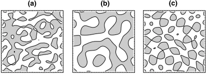
and parabolic lines (where H¼0), whose density isdp. Fig. 10shows a sample of the three types of

line morphology.

The density of zero lines was computed by Longuet–Higgins [28] to be

dz¼

K2

2pffiffiffi2 ð55Þ

and the corresponding line crossing density is_{ffiffiffiffiffi}

K2

p

=ppffiffiffi2, also shown in [28], and also following from BuffonÕs relation. This density is smaller than

dL by a factor of p=2. The density of parabolic lines of an isotropic gaussian random surface can be shown to be [55]

dp¼

2pffiffiffi5Eð4=5Þ 3p

ffiffiffiffiffi

K6 K4

r

¼0:55920 ffiffiffiffiffi

K6 K4

r

; ð56Þ Fig. 9. Venn diagram showing the fractions of different

where E denotes the complete elliptic integral of the second kind [56], and the spectral factor_{ffiffiffiffiffiffiffiffiffiffiffiffiffi}

K6=K4

p

is the square root of that for umbilic points (50). Numerically, this is very close to the L line density, although they are not equal, as dis-cussed above for C points and CTpoint crossings. Mathematically, the difference comes about since

S3¼pxqyqxpy¼0on an L line, where the

sec-ond term is the product of independent random variables, whereas on a parabolic line,

H¼fxxfyyfxy2 ¼0, where the second term is the

square of a random variable.

This difference might appear to be small as far as the L and parabolic densities are concerned, but leads to rather strong differences in the forms of the two sets of line patterns, and the ensuing morphologies of regions of RH and LH in polar-ization fields, and positive and negative gaussian curvature on random surfaces. Morphologically, L lines are closer to zero contour lines than parabolic lines, as may be seen in Fig. 10. This may be seen more clearly in the probability distribution of the values ofS3, f and H – the L lines, zero contour

lines and parabolic lines are the zeros of these functions. The distribution of S3 is symmetric about 0from (A.16), so the L lines partition the plane into equal areas of LH and RH polarization, just as the zero lines of the gaussian distributed f partition the plane into equal areas of f >0and

f <0. However, Longuet–Higgins [29] derived the probability distribution of the gaussian curvature (Eq. (7.14)), which is asymmetric, and in the present notation is given by

PðHÞ ¼ 4

K4pffiffiffi3exp 4H

K4

1HðHÞerf ffiffiffiffiffiffiffi 6H K4

s !!

:

ð57Þ

Although the mean curvature hHi ¼0, the frac-tion of the plane whereHis positive is less than 1/ 2,

hHðHÞi ¼1 1ffiffiffi 3

p ¼0:42265<1

2: ð58Þ

The symmetry of pðS3Þ and pðfÞ imply that the

regions of RH and LH polarizations, and positive and negative regions off, in a random field, are at the percolation threshold [57–59], and there is an infinite, ÔpercolatingÕ L line or zero contour (this does not mean that there cannot be finite loops as well, as in the figures). This contrasts with the asymmetric distribution of H, where generically there are isolated islands of positive curvature, surrounding each extremum (either maximum or minimum), surrounded by a sea of negative cur-vature, which is evident from Fig. 10(c). Each connected region of positive curvature contains exactly one extremum, and the distribution of ex-trema is statistically stationary and isotropic [28].

Acknowledgements

I am grateful to M.V. Berry, J.H. Hannay and J.F. Nye for invaluable discussions, and to I. Freund and M.S. Soskin for useful correspon-dence. This work was supported by the Lever-hulme Trust.

Appendix A. Isotropic gaussian random polariza-tion fields

The gaussian random polarization fields used to derive the results in Section 5 are very simple – each of the complex cartesian componentsEx;Eyis

a circular gaussian random function, of the type normally considered in speckle patterns [44,45], and in the properties of wave dislocations in scalar fields [19], on which the present discussion is based. Each scalar component is a sum of plane Fig. 10. Comparison of the morphology of three types of line in

wave components (neglecting the monochromatic time dependence and paraxialz-dependence)

El¼

X

K

aKexpðiðKRþ/l;KÞÞ; l¼x;y; ðA:1Þ

where theKare transverse wavenumbers, isotropic in direction in thex,yplane, the/l;Kare uniformly

random phases (labelled by l and K) and aK are

spectral factors depending only on the length

K¼K, ensuring that the fields (A.1) are isotropic. The sets of phases f/x;Kg;f/y;Kg are independent

so Ex;Ey are completely independent. All of the

polarization is pure in this model since the fields are monochromatic, and all randomness is spatial. The fields (A.1) are statistically stationary and ergodic, so all spatial averages over R can be re-placed by ensemble averages (over the /_K), de-noted byhi; therefore

hExEyi ¼0: ðA:2Þ

From (6), the field may be rewritten in terms of circular componentsw_R;w_L, and, from (A.2),

hw_Rw_Li ¼0: ðA:3Þ

It may be shown that the above definition of the random Efield is equivalent to

E¼X

K

aKdKexpðiðKRþ/KÞÞ; ðA:4Þ

whereaKand/Kare as above, anddKis a random

complex polarization vector for each K, repre-senting a point chosen at random on the Poincaree sphere,

dK¼4 cosðð aK=2ÞexpðibK=2Þ;

sinðaK=2ÞexpðibK=2ÞÞ; ðA:5Þ

where aK and bK are the angles on the Poincaree

sphere, as defined in the text below Eq. (15), and the factor 4 is for normalization.

Denoting any one of identically distributed and independent real gaussian random fieldspx,qx,py, qy, RewR, ImwR, RewL and ImwL byf:

hf2i ¼1 2

X

K

a2_K¼ Z

d2KPðKÞ

2pK ; ðA:6Þ

where the second equality follows assuming that the K are sufficiently finely spaced that the sum may be replaced by an integral, and PðKÞ is the

radial power spectrum. The two-dimensional Fourier transform of the power spectrum, by the Wiener–Khintchine theorem, is the autocorrela-tion funcautocorrela-tionCðRÞ, also defined by

CðRÞ ¼ hfð0ÞfðRÞi: ðA:7Þ Note that the cross correlations corresponding to the averages Eqs. (A.2), (A.3) are always 0.

Thenth moment ofKwith respect to the radial power spectrumPðKÞis denotedKn; without loss

of generalityPðKÞis normalized, soK0¼1.px,py, qx,qy, and their first derivatives are all independent

(this also applies tonR; gR; nL andgL) and again

denoting any of the fields byf:

hf2i ¼K0¼1;

hf_x2i ¼ hf_y2i ¼K2 2 :

ðA:8Þ

Because of this independence, the normalized probability density function of each of these fields is

Pðf;fx;fyÞ ¼PðfÞPðfxÞPðfyÞ

¼ 2

ð2pÞ3=2K2

exp f

2

2 2ðf2

x þf 2 yÞ K2

!

:

ðA:9Þ

The statistical model for random surfaces is equivalent to any one of the fields denoted by f here [28,25]. It should be noted that [28,25] use the notationMnforKn.

Three particular spectra which the results apply to are the following:

• Disk spectrum. This is a polarization speckle

pattern from a uniformly illuminated circular scatterer, with radius r and distance L from the plane; for wavelength k, writing Kd ¼2p= K¼2pr=kD, its power spectrum is a radial step function, so

Kn;disk¼

2Kn d

2þn ðA:10Þ

and

CdiskðRÞ ¼

2J1ðKdRÞ

KdR ; ðA:11Þ

whereJ1denotes the first order Bessel function.

speckle theory [45,44], and its phase singulari-ties have been well-studied [22].

• Ring spectrum. As above, but the scatterer is

now a ring of negligible thickness; all of theK vectors therefore have the same length (the power spectrum is ad-function), and

Kn;ring¼Kdn ðA:12Þ

and

CringðRÞ ¼J0ðKdRÞ; ðA:13Þ

whereJ0 denotes the zeroth-order Bessel func-tion.

• Gaussian spectrum. This is the field from a

gaussian scatterer, with standard deviationKr,

so

Kn;gauss¼2n=2 n

2 !K

n

r ðA:14Þ

and

CgaussðRÞ ¼exp

K

2 rR

2

2

: ðA:15Þ

The statistics of scalar wave singularities with these spectra were described in [11]. It is pos-sible to show, using this model, that the prob-ability distribution PðSiÞ of the Stokes

parametersSi; i¼1;2;3;is

PðSiÞ ¼

expðjSij=2Þ

4 ; ðA:16Þ

agreeing with the calculations of [48–50].

Appendix B. Calculations of singularity densities

In order to calculate the statistical density of C points (including C points of certain types (RH or LH, star, lemon or monstar, elliptic or hyper-bolic)), we use the fact that the gaussian random field E (A.1), (A.4) is ergodic, and replace the spatial integral in (35) with ensemble averaging, so the densitydC of C points is

dC¼hdðS1ÞdðS2ÞjDIji: ðB:1Þ

It is easier to evaluate (B.1) using the phase pa-rameters T1;T2 instead of the Stokes parameters,

since the phase parameters are invariant with re-spect to rotations of the plane. Also, the density of

any particular type of C point may be evaluated, with an appropriate step H-function on the mor-phological parameters,S3,DI,DL,DC, which is

de-noted for now simply byH, so, generalizing (B.1),

dC;type¼ dðT1ÞdðT2ÞjT1xT2y

T2xT1yjH

: ðB:2Þ As in other derivations of singularity densities [7,11,19], the calculation is simpler if an appropriate coordinate system is chosen to start with; we will representp;qin polar coordinates as (p,h0), and (q,

h0þh). The phase parametersT1;T2, their deriva-tives, and the signs of the morphological parameters are unchanged whenh0is averaged in (B.2), so

dC;type¼

8

p

Z 1

0

dp

Z 1

0

dq

Z 2p

0

dhpqdðp2q2Þ

dð2pqcoshÞ expð2ðp2þq2ÞÞI1;

ðB:3Þ where I1 represents all of the integrals involving first derivatives, including H. The d-functions are easy to integrate (with respect toqandh), and the integral becomes

dC;type¼

16

p

Z 1

0

dp p 2

4p3 expð4p 2_ÞI

1ðq¼p;cosh¼0Þ

ðB:4Þ and the notation I1ðq¼p;cosh¼0Þ is obvious. cosh has

two zeros in the range 06_h6_{2p, the first}

(h¼p=2) when p;q are RH, the other LH. The distributions of C points of any other type are the same whether the points are RH or LH, and it will be assumed in the following that the type does not involve handedness.

The jacobian jT1xT2yT2xT1yjnow simplifies

jT1xT2yT2xT1yj ¼4p2jpx;xpy;yþpx;xqx;y

py;yqy;xþqx;xqy;y

px;ypy;xpx;yqx;x

qx;yqy;xþpy;xqy;yj: ðB:5Þ

Rewriting the first derivatives as a vector

V¼2=pffiffiffiffiffiK2ðpx;x;px;y;py;x;py;y;qx;x;qx;y;qy;x;qy;yÞ;

gaussian), is equal toðK2=4Þ 4

jVNVj, withNthe 88 symmetric matrix with entries 0,1=2, from (B.4). Therefore

dC;type¼

16

p K2

4p4

Z 1

0

dp pexpð4p2Þ

Z

d8VjVNVjexpðV2Þ: ðB:7Þ

Now we perform a linear transformation V! W¼CV with C an orthogonal matrix diagonal-izing N:

CTNC¼diagf1;1;1;1;0;0;0;0g: ðB:8Þ

Such a C can always be found because N is real symmetric. The jacobian of this transformation is 1 since C is orthogonal. Defining atype¼2p=

K2dC;type, after the transformation, we may

write

atype¼ 1

p4

Z

d8WjW2 1 þW

2

2 W

2 3

W₄2jexpðW2ÞHW ðB:9Þ

where any expression inHhas been appropriately changed to theWicoordinates. The total density of

C points may therefore be confirmed by taking

HW ¼1 always in (B.9). By transforming W1;. . .;W6 to

W1¼rcoshcos/1;

W2¼rcoshsin/1;

W3¼rsinhcos/2;

W4¼rsinhsin/2;

W5¼rucos/3;

W6¼rusin/3;

06_{r;u<1; 0}6_h6_p=2;

06_/1;/2;/36_2p;

ðB:10Þ

with jacobian r5_{usinð2hÞ=2. With H}

W ¼1, this

integral can easily be shown to be 1, confirming that dC¼K2=2=p, justified in Eq. (41) a different

way. Otherwise,W7;W8may be integrated (they do

not appear in any of the morphological parame-ters), and

atype¼ 1 2p3

Z 1

0

dr

Z 1

0

du

Z p=2

0

dh

Z

d3/r7usin 2hjcos 2hj

expðr2_ð1þu2_{ÞÞH; ðB:11Þ}

where the morphological parameters, in terms ofr,

h,/1,/2,/3,u, are written

DIW¼cos 2h;

DLW¼1528 cos 2hþ11 cos 4h

4 cosð3/₁þ/₂Þsin 2hð1þcos 2hÞ; ðB:12Þ

DCW¼cos22h2u2ð1cosð/1þ/2 2/3Þsin 2hÞ;

where overall positive multipliers have been ig-nored. Note that onlyDCinvolvesu. The star type

points are those with DI<0, which from (B.11),

(B.12) has astar¼1=2, implying that alemonþ

amonstar ¼1=2. In the following, it is convenient to change the/iangles to/L¼3/1þ/2,/C¼/1þ /22/3, /¼/3=2, which may be done with

ja-cobian 1. Out of the original/ivariables,DLWnow

depends only on/L,DCW only on/C.

The total fraction of lemon type is found using the fact thatDL<0for lemons; DLW in (B.12) is

independent ofr,u,/, and/_C, so integrating these from (B.11) is easy, and gives

alemon ¼1

p

Z p=2

0

dh

Z 2p

0

d/Lsin 2hjcos 2hjHðDLWÞ

¼ 18 100þ

2

p

Z p=4

arccosð3=pffiffiffiffi10Þ

dhsin 2hcos 2h

arccos 1528 cos 2hþ11 cos 4h 4 sin 2hð1þcos 2hÞ

!

¼ 18 100þ

1

p

Z 4=5

0

dt tarccos 428tþ22t

2

4ð1þtÞpffiffiffiffiffiffiffiffiffiffiffiffi1t2

!

¼0:44721: ðB:13Þ

integration. This derivation is similar to that for the fraction of lemon umbilic points in [25], Section 4.

The corresponding calculation for the elliptic (E) type, for whichDC>0, is similar. After

inte-grating outr,/and/L, we have

aE ¼6

p

Z p=2

0

dh

Z 2p

0

d/C

Z 1

0

du u

ð1þu2_Þ4

sin 2hjcos 2hjHðDCWÞ

¼ 3 2p

Z p

0

dh0

Z 2p

0

d/C

Z 1

0

dvsinh

0_jcos

h0j ð1þvÞ4

H 1sin2h02vð1cos/Csinh0Þ

!

;

ðB:14Þ where v¼u2_{, h}0_{¼2h. Therefore, in h}0_{, the}

integrand is symmetric about p=2, that is, in index (from the form ofDIW), soaE;star¼aE;lemonþ aE;monstar. Taking advantage of this symmetry, we

can substitutes¼sinh0, and integratev:

aE ¼3

p

Z 1

0

ds

Z 2p

0

d/C s

3

1 8ð1scos/CÞ 3

ð3s2_2scos/ CÞ

3

! ¼1

2; ðB:15Þ

where the final integration is straightforward. This result implies that 1=2¼aE¼aH¼2aE;star,

etc.

The final density calculation is that of the el-liptic lemons; although the total fraction of elel-liptic lemons and monstars is half, they are not neces-sarily in the same proportion as they are overall. Therefore, after integrating out r and / from (B.11)

aE;lemon ¼

3

p2

Z p=2

0

dh

Z 2p

0

d/L

Z 2p

0

d/C

Z 1

0

du u

ð1þu2_Þ4 sin 2hjcos 2hj

HðDCWÞHðDLWÞ

¼0:23481; ðB:16Þ

where the final numerical result is arrived at from transformations similar to those used foralemon,aE,

and the other fractions may be derived from those found here.

We now turn our attention to L lines, whose average density, by stationarity and ergodicity, can be found from Eq. (37), giving

dL¼dðS3ÞjrS3j: ðB:17Þ

Now, p andq may be transformed to polar coor-dinates as before, and integrate h0, giving

dL ¼8

p Z 1 0 dp Z 1 0 dq

Z 2p

0

dh pqdð2pqsinhÞ

exp2ðp2þq2Þ

Z

d4rpd4rqpðrp;rqÞjrS3j

¼8 p Z 1 0 dp Z 1 0

dqexpð 2ðp2_þq2_Þ

Z

d4rpd4rqpðrp;rqÞjrS3j: ðB:18Þ

Transforming to polars ðp;qÞ ! ðU;/Þ, and us-ing the fact that both p;q are in the same di-rection (relabelled as the x-direction), jrS3j

becomes

2U

ffiffiffiffiffiffiffiffiffiffiffiffiffiffiffiffiffiffiffiffiffiffiffiffiffiffiffiffiffiffiffiffiffiffiffiffiffiffiffiffiffiffiffiffiffiffiffiffiffiffiffiffiffiffiffiffiffiffiffiffiffiffiffiffiffiffiffiffiffiffiffiffiffi

c2_ðrq yÞ

2

þs2_ðrp yÞ

2

2csrpy rqy

q

; ðB:19Þ

where C, sdenote cos/, sin/, respectively. jrS3j

now only involves the derivatives of the y com-ponents ofp;q, so only these need to be integrated over. Writing these as a vector V¼ ffiffiffiffiffiK2

p

=2 ðpy;x;py;y;qy;x;qy;yÞ, and writingjrS3jas a quadratic

form TK2=2jVNVj 1=2

, the integral becomes

dL¼

4pffiffiffiffiffiffiffiffiffiffiK2=2

p3

Z 1

0

dU U2expð2U2Þ

Z 1

0

d/

Z

d4VjVNVjexpðV2Þ: ðB:20Þ

As before,Vcan be orthogonally transformed to a basis in which N is diagonal, and therefore can easily be integrated, with the result

dL¼p

4 ffiffiffiffiffi

K2

2 r

Similar methods are employed to show that the corresponding density of L lines crossing a straight lineds;1, starting from (38), is

dL;1¼

1 2

ffiffiffiffiffi

K2

2 r

: ðB:22Þ

References

[1] J.F. Nye, Proc. R. Soc. London A 389 (1983) 279. [2] J.F. Nye, Proc. R. Soc. London A 387 (1983) 105. [3] J.F. Nye, Natural focusing and fine structure of light:

caustics and wave dislocations, Institute of Physics Pub-lishing, Bristol, 1999.

[4] J.F. Nye, J.V. Hajnal, Proc. R. Soc. London A 409 (1987) 21.

[5] J.V. Hajnal, Proc. R. Soc. London A 414 (1987) 433. [6] J.V. Hajnal, Proc. R. Soc. London A 414 (1987) 447. [7] M.V. Berry, M.R. Dennis, Proc. R. Soc. London A

457 (2001) 141.

[8] M.V. Berry, in: M.S. Soskin, M.V. Vasnetsov (Eds.), Singular Optics Optical Vortices: Fundamentals and Ap-plications, SPIE, vol. 4403, 2001, p. 1.

[9] I. Freund, Opt. Lett. 26 (2001) 1996.

[10] A.I. Konukhov, L.A. Melnikov, J. Opt. B 3 (2001) S139.

[11] M.R. Dennis, Topological singularities in wave fields, Ph.D. Thesis, University of Bristol, 2002.

[12] I. Freund, Opt. Commun. 208 (2002) 223.

[13] O.V. Angelsky, I.I. Mokhun, A.I. Mokhun, M.S. Soskin, Phys. Rev. E 65 (2002) 036602.

[14] I. Freund, A.I. Mokhun, M.S. Soskin, O.V. Angelsky, I.I. Mokhun, Opt. Lett. 27 (2002) 545.

[15] O. Angelsky, A. Mokhun, I. Mokhun, M. Soskin, Opt. Commun. 207 (2002) 57.

[16] I. Freund, M.S. Soskin, A.I. Mokhun, Opt. Commun. 208 (2002) 57.

[17] J.F. Nye, M.V. Berry, Proc. R. Soc. London A 336 (1974) 165.

[18] M. Vasnetsov, K. Staliunas (Eds.), Optical Vortices, Nova Science, Commack, NY, 1999.

[19] M.V. Berry, M.R. Dennis, Proc. R. Soc. London A 456 (2000) 2059 (errata 456 3059).

[20] M.V. Berry, J. Phys. A: Math. Gen. 11 (1978) 27. [21] B.I. Halperin, in: R. Balian, M. Kleeman, J.-P. Poirier

(Eds.), Les Houches Session XXV – Physics of Defects, North-Holland, Amsterdam, 1981, p. 813.

[22] I. Freund, Waves Rand. Med. 8 (1998) 119.

[23] M.R. Dennis, Local properties and statistics of phase singularities in generic wavefields, in: M.S. Soskin, M.V. Vasnetsov (Eds.), Singular Optics Optical Vortices: Fundamentals and Applications, SPIE, vol. 4403, 2001, p. 13.

[24] M.R. Dennis, J. Phys. A: Math. Gen. 34 (2001) L297.

[25] M.V. Berry, J.H. Hannay, J. Phys. A: Math. Gen. 10 (1977) 2083.

[26] I.R. Porteous, Geometric differentiation: for the intelli-gence of curves and surfaces, second ed., Cambridge University Press, Cambridge, MA, 2001.

[27] M.S. Longuet-Higgins, Trans. R. Soc. A 249 (1957) 321.

[28] M.S. Longuet-Higgins, Philos. Trans. R. Soc. A 250(1957) 157.

[29] M.S. Longuet-Higgins, Proc. Cambridge Philos. Soc. 54 (1957) 439.

[30] R.D. Ray, J. Mar. Syst. 28 (2001) 1.

[31] A.S. Thorndike, C.R. Cooley, J.F. Nye, J. Phys. A: Math. Gen. 11 (1978) 1455.

[32] N.D. Mermin, Rev. Mod. Phys. 51 (1979) 591. [33] R. Penrose, Ann. Hum. Gen. 42 (1979) 435.

[34] P.A.G. Scheuer, J.H. Hannay, P.J. Hargrave, Mon. Not. R. Astr. Soc. 180(1977) 163.

[35] D. Brewster, Philos. Mag. 31 (1847) 444.

[36] G. Horvath, J. Gal, I. Pomozi, Naturwissenschaften 85 (1998) 333.

[37] M. Born, E. Wolf, Principles of Optics, Pergamon Press, Oxford, 1959.

[38] In the mathematical language of fibre bundles, the Poincaree sphere is the image of the three-sphere (with coordinates 1= ffiffiffiffiffiS0

p

(px, py, qx, qy)) under the Hopf map (Hopf fibration), and the Hopf circles are all those points which have different rectifying phases v0, but are otherwise the same. The phase sphere is similar, but with Hopf circles parameterised byc0; the two different spheres are related by exchanging py and qx in four-dimensional space.

[39] E. Majorana, Nuovo Cimento 9 (1932) 43. [40] J.H. Hannay, J. Mod. Opt. 45 (1998) 1001.

[41] V.I. Arnold, Mathematical methods of classical mechanics, second ed., Springer, Berlin, 1989.

[42] M.V. Berry, in: G. Iooss, R.H.G. Helleman, R. Stora (Eds.), Les Houches Lecture Series Session XXXVI, North-Holland, Amsterdam, 1983, p. 171.

[43] M.V. Berry, J. Phys. A: Math. Gen. 8 (1975) 566. [44] J.C. Dainty, Prog. Opt. 14 (1976) 1.

[45] J.W. Goodman, in: J.C. Dainty (Ed.), Laser speckle and related phenomena, Springer, Berlin, 1975, p. 9.

[46] R. Barakat, Opt. Acta 32 (1985) 295. [47] D. Eliyahu, Phys. Rev. E 47 (1993) 2881. [48] R. Barakat, J. Opt. Soc. Am. A 4 (1987) 1256. [49] A.F. Fercher, P.F. Steeger, Opt. Acta 28 (1981) 443. [50] D. Eliyahu, Phys. Rev. E 50 (1994) 2381.

[51] I. Freund, M. Wilkinson, J. Opt. Soc. Am. A 15 (1998) 2892.

[52] J.P. Hansen, I.R. McDonald, Academic Press, New York, 1986.

[53] M.R. Dennis, I. Freund, C point screening in random optical ellipse fields, Opt. Lett. (August) (2002), submitted. [54] H. Solomon, Geometric Probability, SIAM, Arrowsmith,

Bristol, 1978.

[56] M. Abramowitz, I.A. Stegun (Eds.), Handbook of Math-ematical Functions, Dover, New York, 1965.

[57] R. Zallen, H. Scher, Phys. Rev. B 4 (1971) 4471.

[58] A.V. Milovanov, G. Zimbardo, Phys. Rev. E 62 (2000) 250.