Strain transducers for active control lumped parameter model

(1)

Strain Transducers for Active Control - Lumped Parameter Model -

Y. Aoki, P. Gardonio and S.J. Elliott

(2)

SCIENTIFIC PUBLICATIONS BY THE ISVR

Technical Reports are published to promote timely dissemination of research results

by ISVR personnel. This medium permits more detailed presentation than is usually acceptable for scientific journals. Responsibility for both the content and any opinions expressed rests entirely with the author(s).

Technical Memoranda are produced to enable the early or preliminary release of

information by ISVR personnel where such release is deemed to the appropriate. Information contained in these memoranda may be incomplete, or form part of a continuing programme; this should be borne in mind when using or quoting from these documents.

Contract Reports are produced to record the results of scientific work carried out for

sponsors, under contract. The ISVR treats these reports as confidential to sponsors and does not make them available for general circulation. Individual sponsors may, however, authorize subsequent release of the material.

COPYRIGHT NOTICE

(3)

UNIVERSITY OF SOUTHAMPTON

INSTITUTE OF SOUND AND VIBRATION RESEARCH

SIGNAL PROCESSING AND CONTROL GROUP

Strain Transducers for Active Control

- Lumped Parameter Model -

by

Y Aoki, P. Gardonio and S.J. Elliott

ISVR Technical Memorandum No: 970

August 2006

Authorised for issue by Prof. R. Allen

Group Chairman

(4)

List of Figures

1.1 Smart panel with a piezoelectric patch actuator and a velocity sensor at its center for the implementation of a direct velocity feedback control loop that generates active damping . . . 7

2.1 Physical arrangement of test rigs, which consist of an acoustic cavity with rigid walls and a baffled clamped smart panel, excited by a transverse point force generated by a shaker . . . 11 2.2 Moments excitation generated by a piezoelectric patch that is bonded on the

bottom side of the panel, when the applied voltage has the same polarity as the poling voltage. . . 13 2.3 Block diagram of the direct velocity feedback control system . . . 13 2.4 The Bode plot (left) and the Nyquist plot(right) of the open loop FRF of a

closely located velocity sensor and a square piezoelectric actuator(solid line), and the predicted phase lag (dashed line) . . . 16 2.5 Definition of the stability coefficient (δ0) and the control performance coefficient(δrk) 18

2.6 Maximum reduction index Rk with reference to the control ratio δ0k . . . 18

3.1 Schematic representation of distributed mass model . . . 20 3.2 The Bode plot (top) and the Nyquist plot (bottom 1 by 2 array) of the open

loop FRF between the ideal velocity sensor and either the massless piezoelectric actuator (faint line, left), or the lightweight piezoelectric actuator (dotted line, right) . . . 22 3.3 Schematic representation of the actuator stiffness model with single pair of

springs . . . 23 3.4 Schematic representation of the lumped spring model of the actuator patch

with the notation of the forces and displacements at the connecting points between the lumped spring and the smart panel in x-direction (top) and y-direction(bottom) . . . 28 3.5 Schematic representation of the actuator stiffness model with multiple pairs of

springs . . . 28 3.6 The Bode plot (top) and the Nyquist plot (bottom 1 by 2 array) of the open

loop FRF of the ideal velocity sensor and the piezoelectric actuator without (faint line, left) and with (dotted line, right) stiffness effect of the piezoelectric actuator . . . 29 3.7 Actuation moment (solid black line) and total moment including the stiffness

(7)

3.8 The Bode plot (top) and the Nyquist plot (bottom 1 by 2 array) of the open loop FRF between the ideal velocity sensor and the piezoelectric actuator without (faint line, left) and with (dotted line, right) inertia and elastic effects of the piezoelectric actuator . . . 32 3.9 Internal structure of tri-shear piezoelectric sensing accelerometer 352C67 . . . 33 3.10 Schematic representation of the piezoelectric accelerometer transducer, which

is modeled as a single degree-of-freedom system . . . 34 3.11 Transfer function between the acceleration of the panel at the sensor position

and the voltage signal output of the accelerometer . . . 36 3.12 Schematic representation of a piezoelectric accelerometer transducer, and the

notation of the forces and displacement at the connecting points between the elements of the accelerometer and the smart panel . . . 37 3.13 The Bode plot (top) and the Nyquist plot (bottom, 1 by 2 array) of the open

loop FRF between the ideal accelerometer sensor and the practical piezoelectric actuator (faint line), the open loop FRF between the integrated signal from the accelerometer sensor and the practical piezoelectric actuator (dotted line, right) . . . 40 3.14 The Bode plot (top) and the Nyquist plot (bottom, 1 by 2 array) of simulated

open loop FRF using the plate-actuator fully coupled model (solid line, left), and measured open loop FRF between the input signal to the piezoelectric actuator and the output signal obtained by laser vibrometer (dotted line, right) 43 3.15 The Bode plot (top) and the Nyquist plot (bottom, 1 by 2 array) of the

simu-lated open loop FRF using the plate-actuator-sensor fully coupled model (solid line, left), and the measured open loop FRF between the input signal to the piezoelectric actuator and the digitally integrated output signal obtained by the accelerometer sebsor (dotted line, right) . . . 44

4.1 The Bode plot (top) and the Nyquist plot (bottom 2 x 2 array) of the open loop FRF between the ideal velocity sensor and various size actuators; Case 1: 20x20mm (faint line, left top), Case 2: 30x30mm (dotted line, right top), Case 3: 40x40mm (dash-dotted line, left down), Case 4: 50x50mm (dashed line, right down) . . . 47 4.2 The Bode plot (top) and the Nyquist plot (bottom 2 x 2 array) of the open

loop FRF between the integrated signal of the accelerometer sensor and vari-ous size actuators; Case 1: 20x20mm (faint line, left top), Case 2: 30x30mm (dotted line, right top), Case 3: 40x40mm (dash-dotted line, left down), Case 4: 50x50mm (dashed line, right down) . . . 48 4.3 Flexural wavelength with reference to frequency . . . 49 4.4 Maximum vibration reduction at 1st(blue solid line), 4th (black dotted line),

8th (red dot dashed line), and 11th resonance (green dashed line) with refer-ence to the size length, using the ideal velocity sensor-actuator pair (left) or accelerometer sensor-actuator pair (right) . . . 49 4.5 The Bode plot (top) and the Nyquist plot (bottom 2 x 2 array) of the open loop

(8)

4.6 The Bode plot (top) and the Nyquist plot (bottom 2 x 2 array) of the open loop FRF between the integrated signal of the accelerometer sensor and various thickness actuators; Case 1: 0.001mm (faint line, left top), Case 2: 0.25mm (dotted line, right top), Case 3: 0.5mm (dash-dotted line, left down), Case 4: 1.0mm (dashed line, right down) . . . 52 4.7 Maximum vibration reduction at 1st(blue solid line), 4th (black dotted line),

8th (red dot dashed line) ,and 11th resonances (green dashed line) with refer-ence to the thickness of the actuator using the ideal velocity sensor-actuator pair (left) or using accelerometer sensor-actuator pair (right) . . . 53 4.8 The Bode plot (top) and the Nyquist plot (bottom 2 x 2 array) of the open

loop FRF between the ideal velocity sensor and various size and thickness actuators; Case 1: 20x20mm 1.125mm (faint line, left top), Case 2: 30x30mm 0.5mm (dotted line, right top), Case 3: 40x40mm 0.28mm (dash-dotted line, left down), Case 4: 50x50mm 0.18mm (dashed line, right down) . . . 55 4.9 The Bode plot (top) and the Nyquist plot (bottom 2 x 2 array) of the open

loop FRF between the integrated signal of the accelerometer sensor and various size and thickness actuators; Case 1: 20x20mm 1.125mm (faint line, left top), Case 2: 30x30mm 0.5mm (dotted line, right top), Case 3: 40x40mm 0.28mm (dash-dotted line, left down), Case 4: 50x50mm 0.18mm (dashed line, right down) . . . 56 4.10 Maximum vibration reduction at 1st(blue solid line), 4th (black dotted line),

8th (red dot dashed line), and 11th resonance (green dashed line) with reference to the size of the actuator using the ideal velocity sensor-actuator pair (left) or using accelerometer sensor-actuator pair (right) . . . 57 4.11 The Bode plot (top) and the Nyquist plot (bottom 2 x 2 array) of the open

loop FRF between the ideal velocity sensor and the actuator with various offset length; Case 1: no offset (faint line, left top), Case 2: 0.25mm offset(dotted line, right top), Case 3: 0.5mm offset (dash-dotted line, left down), Case 4: 1.0mm offset(dashed line, right down) . . . 59 4.12 The Bode plot (top) and the Nyquist plot (bottom 2 x 2 array) of the open

loop FRF between the ideal velocity sensor and the actuator with various offset length; Case 1: no offset (faint line, left top), Case 2: 0.25mm offset(dotted line, right top), Case 3: 0.5mm offset (dash-dotted line, left down), Case 4: 1.0mm offset(dashed line, right down) . . . 60 4.13 Maximum vibration reduction at 1st(blue solid line), 4th (black dotted line),

8th (red dot dashed line), and 11th resonance (green dashed line) with reference to the offset length, using the ideal velocity sensor-actuator pair (left) or using accelerometer sensor-actuator pair (right) . . . 61

C.1 Strain distribution; (a)unconstrained piezoelectric actuator(Top) and (b) bonded piezoelectric actuator on the panel (bottm) . . . 79 C.2 Stress distribution (top) and its decomposition into passive (bottom left) and

(9)

List of Tables

2.1 Geometric and physical properties of the smart panel . . . 10 2.2 Geometric and physical properties of the the piezoelectric patch actuator . . . 11

3.1 Geometric and physical properties of the accelerometer . . . 39

4.1 Geometric parameter of the piezoelectric patch actuator considered in the para-metric study regarding the actuator size . . . 49 4.2 Geometric parameter of the piezoelectric patch actuator considered in the

para-metric study regarding the actuator thickness . . . 53 4.3 Parameter of the actuator considered in the parametric study regarding the

actuator size and thickness . . . 57 4.4 Geometric parameter of the piezoelectric patch actuator considered in the

para-metric study regarding the offset length . . . 61

(10)

Chapter 1 INTRODUCTION

1.1 Active Structural Acoustic Control

Over past decades noise and vibration effects on human beings have been regarded as signifi-cant problems and the regulations for the maximum acoustic and vibration levels have become more and more stringent. Especially for both land and air transportation vehicles, the con-trol of vibration and sound transmission through lightly damped panels is an important issue, since it might result in discomfort.

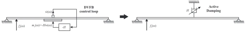
[image:10.612.82.511.512.568.2]

In general, vibration and sound radiation control is achieved with passive treatments, which offer efficient results at high audio frequencies. However, passive approaches tend to have limited performance at low audio frequencies and require relatively bulky and heavy treatments[1]. Alternatively, at low audio frequencies, active vibration control techniques can be employed to reduce the sound radiation through thin structures. The low frequency response of lightly damped thin structures is characterized by well separated and sharp resonances. In the vicinity of resonance frequencies active damping control tends to be effective[1],[2]. Direct velocity feedback (DVFB) control is a simple way to implement ac-tive damping control[1],[3]. As schematically shown in Figure 1.1, when DVFB control is implemented, the control actuator exerts a control action directly proportional to the oppo-site of the velocity at the error sensor, thus it generates active damping.

Figure 1.1: Smart panel with a piezoelectric patch actuator and a velocity sensor at its center for the implementation of a direct velocity feedback control loop that generates active damping

(11)

Elliott et al.[7] have proposed to use arrays of decentralized single channel velocity feedback control systems to generate active damping in panels. Their studies have shown that arrays of direct velocity feedback control systems can be efficiently operated to reduce both the low frequency vibration of the panel and its sound radiation or transmission. The use of control units with small piezoelectric patch actuators and accelerometer sensors at their centers has been considered in order to obtain compact and lightweight panels[8]-[10]. The velocity sensor detects the transverse vibration and the piezoelectric patch actuator exerts line moments along the edges[11], so that this control unit is neither collocated nor dual[5]. Thus, the plant responses of the decentralized control units are not guaranteed to be positive real at all frequencies[6]. As a result, the decentralized control loops are stable only for a limited range of control gains[2], [6]. This limits the generation of active damping on the structure and thus the vibration reduction and sound transmission[8]-[10]. It is therefore crucial to improve the collocation and duality properties of the velocity sensor and the piezoelectric patch actuator pair in order to develop more stable and robust feedback control loops, which produce the desired levels of active damping on smart panels.

1.2 Scope and Objectives

This report presents simulations and experimental results regarding the modeling of a smart panel, which consists of a rectangular panel with the dimensionslx×ly = 414mm ×314mm

and a single control unit. This control unit is composed of three main components: (1) an accelerometer sensor that detects out-of-plane acceleration, (2) a piezoelectric patch actuator that acts as the secondary controlling source, and (3) an analogue constant gain feedback controller, that connect the accelerometer sensor to the piezoelectric patch actuator. The piezoelectric transducer is bound on one sides of the panel, while the accelerometer sensor is attached on the other side in correspondence to the center of the actuator. The smart panel is mounted on a rigid frame positioned on the top open side of a rectangular cavity with thick rigid walls.

The three main objectives of this report are:

1. to build a mathematical model of smart panel, which separate the various effects of the local response of the sensor-actuator unit;

2. to validate the model by experiments;

3. to investigate the configuration of the control unit, which maximize the stability and performance of the control system.

(12)

carried out in order to achieve the thirdobjective listed above. Both the Bode and the Nyquist plots of the open loop sensor-actuator FRFs are used to investigate the stability of the feed-back loop, which is assessed with reference to Nyquist stability criterion. The performance of the control unit is investigated in term of the maximum vibration reduction at first few resonances. A simple formula is proposed, which gives these maximum vibration reductions at resonance frequencies from the Nyquist plot of the open loop sensor-actuator FRFs.

1.3 Structure of the Report

(13)

Chapter 2 ACTIVE CONTROL AND

STABILITY

The study presented in this report considers a rectangular thin aluminium panel with dimen-sions 414mm x 314mm and 1mm thickness. As shown in Figure 2.1, the panel is mounted on a rigid frame, which is positioned on the top open side of a rectangular cavity with rigid walls. This test rig has been designed in such a way to get sound radiation into the open space only from the top side of the panel. The plate is driven into motion by a shaker that generate point forcefp at the position (xp,yp) = (62.1mm, 138.2mm). It is assumed that the

radiated acoustic sound pressure has no effect on the vibration of the panel. The geometry and physical properties of the plate are given in Table 2.1.

The panel is equipped with one feedback control unit that consists of a closely located accelerometer sensor and a square piezoelectric actuator. The piezoelectric actuator has a dimension of 25mm x 25mm x 0.5mm and is fixed on the inner side of the panel by a thin bonding layer of glue. The center position of the piezoelectric patch, where the error sensor is also located, is situated at (xc, yc) = (136.6mm, 222.9mm). The physical properties and

geometry of the piezoelectric patch considered in this study are summarized in Table 2.2.

Table 2.1: Geometric and physical properties of the smart panel

parameter value

Dimensions lx x ly = 414mm x 314mm

Thickness hs = 1mm

Density ρs=2700 kg/m3

Young’s Module Es=7.2x109 N/m2

Poisson’s Ration νs=0.33

(14)

Figure 2.1: Physical arrangement of test rigs, which consist of an acoustic cavity with rigid walls and a baffled clamped smart panel, excited by a transverse point force generated by a shaker

Table 2.2: Geometric and physical properties of the the piezoelectric patch actuator

parameter value

Dimensions ax x ay = 25mm x 25mm

Thickness hpzt = 0.5mm

Center Position xc x yc = 0.33lx x 0.71ly

Density ρpzt=7600 kg/m3

Young’s Module Epzt=6.1x109N/m2

Poisson’s Ration νpzt=0.31

Strain Constant d31=268x10−12 m/V

Actuation Constant cα=1.226x10−3 N/V

(15)

2.1 DVFB Control

When the panel is excited by the primary excitationfpand the control momentsmc, generated

by an ideal massless piezoelectric actuator, the phasor of the velocity in z-direction at the sensor position ˙wc can be written using the following mobility expression:

˙

wc =Ycpfp+Ypccmc, (2.1)

where Ycp is the mobility function between the primary excitation and the velocity at the

control sensor, and Yp_cc is a 4-element row vector with the mobility functions between the control moments along the edges of the actuator and the control velocity:

Yp_cc=_⌊ Ycx1 Ycx2 Ycy1 Ycy2 ⌋. (2.2)

The derivation of the mobility functions is given in Appendix A, and the formula for the mobility functions used in thsi chapter are given in section 1 of Appendix B. In Eq.(2.1),mc

denotes a 4-element column vector with the control moments generated by the piezoelectric patch along the four edges:

mc =

h

mcx1 mcx2 mcy1 mcy2

iT

= mc

h

−1 1 1 ₋1 iT (2.3)

= mcd,

wheremcx1, mcx2,mcy1, and mcy2 are respectively the control moment alongy =yc1 between

x= (xc1, xc2), andy =yc2 between x= (xc1, xc2), x=xc1 betweeny = (yc1, yc2), and x=xc2

between y = (yc1, yc2), as shown in Figure 2.2. mc denotes the magnitude of the effective

bending moment per unit length, which is induced by the piezoelectric patch actuator to the panel. The effective momentmc is proportional to the applied voltage across the piezoelectric

actuator Vc,

mc =cαVc, (2.4)

wherecα is the piezoelectric constant given in Eq.(C.17). The details regarding the

formula-tion of the effective actuaformula-tion moments is presented in Appendix C.

The response at the error sensor generated by the primary excitation and the Direct Velocity FeedBack (DVFB) control loop can be formulated in terms of the classic disturbance rejection block diagram as shown in Figure 2.3. In this figureH denotes a constant feedback gain, and Vc denotes the input voltage signal to the piezoelectric actuator. When the DVFB

control loop is implemented, the control voltageVc is defined as follows:

Vc =−Hw˙c. (2.5)

Thus, the actuator induced momentmc is given by:

mc =cαVc =−cαHw˙c. (2.6)

Therefore, the velocity at the sensor location ˙wc can be calculated as:

˙

wc =

Ycpfp

1 +GsH

, (2.7)

whereGsdenotes the transfer function between the error sensor and the piezoelectric actuator:

(16)

z y

my1

my2 mx2

mx1

xc1 xc2 yc2

yc1

[image:16.612.214.382.443.621.2]

x

Figure 2.2: Moments excitation generated by a piezoelectric patch that is bonded on the bottom side of the panel, when the applied voltage has the same polarity as the poling voltage.

V

c

-H

S

+

Y

_cp

f

p

w

c

G

s

(17)

2.2 Open Loop Frequency Response Function

In feedback control loops, the control performance is strongly linked to the stability of the control loop. In principle, if the control loop is unconditionally stable, very high control gains can be implemented, such that a perfect cancelation can be generated at the control point. In contrast, when the system is only conditionally stable, a limited range of control gains can be implemented, which may lead to modest vibration reductions at the sensing position.

The stability of a control system is commonly assessed by the open loop sensor-actuator FRF, Gc, between the output signal from the velocity sensor ˙wc and the input signal to the

controller:

Gc =GsH. (2.9)

For proportional feedback control, the control functionH is set to unity, H = 1. In this case, the open loop FRF is given by:

Gc =Gs =cαYpccd. (2.10)

Figure 2.4 shows the Bode plot (left) and the Nyquist plot (right) of the predicted sensor-actuator open loop FRF Gc, assuming that the panel is simply supported along four edges.

For the practical damping of the test rig considered in this study, the boundary condition can not be considered neither clamped or simply supported. At lower frequencies up to around 500Hz, the boundary condition is almost clamped on all four edges, and at higher frequencies from around 1kHz, the boundary condition is close to simply supported on all four edges. Therefore, since the stability analysis requires the analysis of the sensor-actuator open loop FRF up to very high frequencies, which means up to 50kHz in this study, the modeling has been carried out considering simply supported boundary condition.

The Bode plot in Figure 2.4 indicates that the amplitude of the sensor-actuator FRF grows when the frequency rises. This is a typical feature of moment-type excitation that is normally encountered with strain actuators[12]. The phase plot indicates that the phase is confined between _±90deg up to about 10kHz, and then a phase lag takes place. This effect is due to the non perfect collocation between the position of the error signal detection at the center of the piezoelectric patch and the bending control excitation at the edges of the piezoelectric patch.

The Nyquist plot in Figure 2.4 is characterized by a series of circles, which are determined by the resonant response of the modes of the plate. In low frequencies the locus starts from vicinity of the origin and moves in the right hand side quadrants. As the frequency rises, the locus tends to drift away from the origin. This is due to the residual effect from the resonant response of neighbor resonances. At low frequencies the modal density is low, so that the residual effect of the neighbor modes is negligible. As the plate modal overlap increases with frequency, the residual effect from the resonant response of neighbor resonances on the resonant response becomes more pronounced, and this effect shifts the locus away from the origin. At higher frequencies the locus enters and goes through the left hand side quadrants in a clockwise rotation. This drifting effect is caused by the phase lag generated by the non-perfect collocation between the sensor and the actuator pair.

The phase lag of the flexural waves Φ is given as the product of the circular frequency ω

and the time delaytb [12] it takes the bending waves, generated at the edges of the piezoelectric

patch, to travel to its center position, at the error sensor location:

Φ = ωtd=

ωds

cb

(18)

where cb denotes the propagation speed of the flexural wave, and ds denotes the distance

between the error sensor and the edge of the patch actuator. As the sensor is situated at the center of the square patch, the distance is given as half of the patch length a:

ds =

a

2. (2.12)

Assuming a single sine wave, the phase velocity of the flexural wavescb is given by the following

formula[13][14]:

cb = 4

s Ds

ρshs

√

ω, (2.13)

whereρs is the density, and hs is the thickness of the panel. Ds denotes the bending stiffnes,

which is given as the product of the module of elasticity Es and the area moment of inertia

per unit width, Is:

Is =

h3 s

12. (2.14)

Thus, using Eq.(2.13), the phase lag Φ can be expressed as follows:

Φ = a 2

√ ω4

s ρshs

Ds

. (2.15)

This equation indicates that the phase lag monotonically increases with reference to the square root of the circular frequency. The progressive phase lag of the open loop FRF brings the control system to a positive feedback velocity loop, rather than negative, so that the system becomes unstable.

Considering that the open loop FRF Gc is defined as the ratio between the velocity and

the applied excitation, not between the the displacement and the excitation, the simulated phase ofGc is 90deg larger than the predicted phase lag given in Eq.(2.15), thus:

Φc =

a

2

√ ω4

s ρshs

Ds −

π

2. (2.16)

The predicted phase lag is plotted in Figure 2.4 by the dashed line, which follows the rough outline of the phase lag of the sensor-actuator open loop FRF.

As a summary, Figure 2.4 highlights the following conclusions.

1. A piezoelectric patch actuator efficiently excites higher frequency resonant modes.

2. As frequencies rises, the locus drifts away from the origin due to the residual effect from the resonant response of neighbor resonances.

3. The sensor-actuator open loop FRF is bound to be positive real only at low frequencies due to the phase lag, which is generated by the non-perfect collocation between the actuation moment along the perimeter of the actuator and the velocity sensing at the center of the actuator.

(19)

101 102 103 104 105 −60

−40 −20

Frequency [Hz]

|G| [dB]

101 102 103 104 105

−360 −180 −90 0 90

Frequency [Hz]

Phase [deg]

−5 0 5

x 10−4

−8 −6 −4 −2 0 2 4 6

8x 10

−4

Figure 2.4: The Bode plot (left) and the Nyquist plot(right) of the open loop FRF of a closely located velocity sensor and a square piezoelectric actuator(solid line), and the predicted phase lag (dashed line)

2.3 Control Performance

As discussed in the introduction chapter of this report, the aim of velocity feedback is to generate active damping, which is particularly effective at resonance frequencies, where in fact the response of the structure is principally controlled by damping. The control performance of the feedback system at thekth _{resonance frequency} _ω

k can be assessed in terms of a factor

ρk, which is given by the ratio between absolute value of the the velocity phasor at the error

sensor without control and with the maximum control gainHmaxthat guarantees the stability:

ρk = |

˙

w(ωk)max control|

|w˙(ωk)no control|

=

Ycp(ωk)fp

1 +HmaxGc(ωk)

1

|Ycp(ωk)fp|

(2.17)

= 1

|1 +HmaxGc(ωk)|

.

According to Nyquist stability criterion, the maximum control gain Hmax is given by the

reciprocal ofδ0:

Hmax=

1

δ0

, (2.18)

whereδ0 denotes the absolute distance between the origin and the FRF, when the locus of the

open loop sensor-actuator FRF crosses the real negative axis at the frequency ω0, as shown

in the Nyquist plot in Figure 2.5:

δ0 = |Gc(ω0)| (2.19)

= ₋Re(Gc(ω0)).

(20)

be approximated by the amplitude δrk, where the kth resonance circle crosses the real axis.

Therefore, Eq.(2.17) can be simplified into the following formula:

ρk ∼=

1

1 + |Gc(ωk)|

|Gc(ω0)|

= 1

1 + δrk

δ0

(2.20)

= 1

1 +δ0k

,

where δ0k = δ_δrk0 denotes the ratio between the amplitude of the k

th _{resonance circle} _δ

rk and

the maximum control gainδ0 in the Nyquist plot of the open loop sensor-actuator FRF. The

index of the maximum vibration reduction Rk that can be generated by the control loop is

defined by the reciprocal of the indicator ρk in the unit of decibel:

Rk = 20 log10

1

ρk

= 20 log₁₀(1 +δ0k). (2.21)

This equation gives the approximate index of the maximum vibration reduction Rk on the

sensor location at the kth _{resonance frequency. This formulation provides a simple approach}

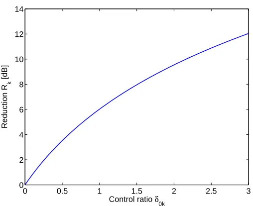
to derive the control effectiveness at low frequency resonances based on either the predicted or measured open loop sensor-actuator FRF of the feedback control system. The index of the maximum vibration reductionRk is plotted in Figure 2.6 for a range of ratios δ0k from 0 to 3.

This plot suggests that it is sufficient to have a ratio of 2 in order to obtain a 10 dB reduction of vibration at the error sensor position. This graph is of great importance since it can be used in combination with the Nyquist plot of the sensor-actuator FRF to assess both the stability and the control performance of a velocity feedback loop at resonance frequencies. In fact, it is sufficient to estimate the ratio δ0k from the Nyquist plot of the open loop sensor-actuator

(21)

−6 −4 −2 0 2 4 6 x 10−4 −6

−4 −2 0 2 4 6

x 10−4

[image:21.612.180.412.81.326.2]

δ_r1 δ₀

Figure 2.5: Definition of the stability coefficient (δ0) and the control performance

coefficient(δrk)

0 0.5 1 1.5 2 2.5 3

0 2 4 6 8 10 12 14

Control ratio δ

0k

Reduction R

k

[dB]

[image:21.612.171.425.446.653.2]

(22)

Chapter 3 MODEL PROBLEM

The mobility model considered in the previous chapter neglected several features of the control system, which can be summarized in the following points:

1. physical passive effects of the actuator and the sensor (mass and stiffness of the actuator, and mass of the sensor)

2. dynamic effects of the sensor (fundamental axial resonance)

3. offset effect due to the mounting method of the piezoelectric patch actuator

Intuitively, the compact and lightweight control system justifies these simplifications. How-ever, it is crucial to investigate the effects of these physical properties on the stability in order to design a feasible actuator-sensor pair with good stability properties. In order to study and assess each effect independently, several models are considered in this chapter. Two fully coupled models are introduced, and these models are experimentally verified.

3.1 Actuator Mass Effect

In this section, the inertia effect of the piezoelectric patch actuator mass is modeled and analyzed. A simple model of this mass effect can be formulated by considering that the mass of the piezoelectric patch is concentrated at its center, where the control sensor is attached. Due to the linearity of the system, the phasor of the velocity at the error sensor ˙wc can be

expressed as follows:

˙

wc =Ycpfp+Yccp mc+Ycmfm, (3.1)

where Ycm is the mobility function between the force generated by the inertia effect of the

actuator fm and the velocity at the error sensor. This force is derived from Newton’s second

law:

fm = −mpztw¨c

= ₋jωmpztw˙c, (3.2)

where mpzt denotes the mass of the piezoelectric actuator. Using Eq.(3.2), Eq.(3.1) can be

written as:

˙

(23)

= Ycp 1 +jωmpztYcm

fp+

1

1 +jωmpztYcm

Yp_ccmc (3.3)

= Yecpfp+Yf p ccmc.

Since the patch actuator is uniformly bonded to the panel, the single lumped mass model can not properly estimate the distributed inertia effect of actuator mass, especially at higher frequencies where the wavelength becomes closer to the patch side dimension. Therefore, instead of a single lumped mass model, a multiple lumped mass model is introduced. The actuator is modeled by a grid of rectangular elements as illustrated in Figure 3.1. The size of these elements has been chosen to be shorter than a quarter of the flexural wavelength at the maximum frequency considered in this study. According to the reference[13], the smallest flexural wavelength is λmin=13.8mm at a maximum frequency of 50kHz. Therefore,

the actuator, with the dimension of 25mm x 25mm, has been subdivided into a grid of 8 x 8 elements, with the dimension 3.125mm x 3.125mm.

m

e

f

pzt i,j

Figure 3.1: Schematic representation of distributed mass model

When inertia effect of the actuator mass is modeled by the multiple elements, the velocity at the sensor position ˙wc is given as follows:

˙

wc =Ycpfp+Yccpmc+Ycmfm, (3.4)

where Ycm is a n2m-element row vector with the mobility functions between the forces

gen-erated by the inertia effects of elemental masses and the control velocity. nm is the number

of the elements in x- and y-directions. f_m is a n2m-element column vector with the forces

generated by inertia effects of lumped masses:

f_m = h f1,1

m fm1,2 · · · fmi,j · · · fmnm,nm

iT

= ₋jωmmw˙m, (3.5)

where fmi,j represents the force due to inertia effect of ith, jth element, and mm denotes the

mass of each element. Assuming that the thickness of the patch is constant, and each element has the same dimension, the mass of each element is given by:

mm =

mpzt

n2 m

. (3.6)

In Eq.(3.5),w˙m is an2m-element column vector with the phasor of the velocities at the centers

of the lumped masses:

˙

wm =

h

˙

w1,1

m w˙m1,2 · · · w˙mi,j · · · w˙mnm,nm

iT

(24)

where ˙wmi,j represents the phasor of the velocity of ith, jth element. Ymp is a n2m-element

column vector with the mobility functions between the primary excitation and the velocities at center of the elements. Ymc is a n2m× 4 matrix with the mobility functions between the

control moments along the edges of the square patch actuator and the velocities at center of the element. Ymm is a n2m ×n2m matrix with the mobility functions between the forces

generated by the inertia effect of the lumped masses and the velocities at the centers of the elements. Substituting Eq.(3.7) into Eq.(3.5), the force vector f_m is given by:

f_m = ₋jωmm(Ympfp+Ymcmc +Ymmfm)

= ₋jωmm[I+jωmmYmm]

−₁

(Ympfp+Ymcmc), (3.8)

where I denote a n2_m_×n2_m identity matrix. Substituting Eq.(3.8) into Eq.(3.4), the control velocity ˙wc can be expressed as:

˙

wc =Yecpfp+Yf p

ccmc, (3.9)

whereYecp and Yf p

cc are given below:

e

Ycp = Ycp−jωmmYcm[I +jωmmYmm]

−1

Ymp (3.10)

f

Yp_cc = Yp_cc₋jωmmYcm[I+jωmmYmm]

−₁

Ymc. (3.11)

Further details regarding the mobility functions used in this section are given in section 2 of Appendix B.

Figure 3.2 compares the simulated open loop FRF between the ideal sensor and the ideal massless piezoelectric actuator with the simulated open loop FRF between the ideal sensor and the lightweight piezoelectric actuator, in which case, Gc is given by:

Gc =cαY˜ p

ccd. (3.12)

(25)

101 102 103 104 −60

−40 −20

[image:25.612.124.477.139.568.2]

Frequency [Hz]

|G| [dB]

101 102 103 104

−360 −180 −90 0 90

Frequency [Hz]

Phase [deg]

−0.5 0 0.5

−0.5 −0.4 −0.3 −0.2 −0.1 0 0.1 0.2 0.3 0.4 0.5

−0.4 −0.2 0 0.2 0.4

−0.4 −0.3 −0.2 −0.1 0 0.1 0.2 0.3 0.4

(26)

3.2 Actuator Stiffness Effect

When the actuator is bonded to the panel, the patch locally increases the stiffness of the structure. In this section the passive elastic effect of the piezoelectric patch actuator is modeled and analyzed. At first, in order to simply assess this passive effect of the actuator, the patch actuator is modeled by a single pair of linear springs, as shown in Figure 3.3. Due to the linearity, when the stiffness of the patch actuator is taken into account, the phasor of the velocity at the error sensor can be expressed as:

˙

wc =Ycpfp+YcMMt, (3.13)

whereYcM denotes a 4-element row vector with the mobility functions between the moments

acting on the edges of the patch actuator and the control velocity. Mt denotes a 4-element

column vector with the moments generated by the piezoelectric actuation and the elastic effect of the lumped springs:

Mt=

h

Mx1 Mx2 My1 My2

iT

, (3.14)

where Mx1, Mx2, My1, and My2 are the total moments generated along y = yc1 between

x= (xc1, xc2), andy =yc2 between x= (xc1, xc2), x=xc1 betweeny = (yc1, yc2), and x=xc2

between y = (yc1, yc2), respectively. When the piezoelectric patch actuator is modeled by a

single pair of springs, the total line moments along the edges are concentrated atxc1+xc2 2 , yc1

,

_x c1+xc2

2 , yc2

,xc1,yc1+₂yc2

, and xc2,yc1+₂yc2

, respectively.

The discretized total moment acting on the panel Mt is defined as the summation of the

discretized effective control actuation momentMc and discretized passive moment generated

by the elastic effect of the actuator patchMk:

Mt=Mc +Mk, (3.15)

whereMc is a 4-element column vector:

Mc =mc

h

−ax ax ay −ay

iT

, (3.16)

whereax anday are respectively the length of the actuator in x- and y-directions. Considering

the coordinate system defined in Figure 3.4, the vectorMk with the passive moment on the

ax

ay

hpzt

Ax _M

y1

My2

Mx1

Mx2

x y z

(27)

panel is given by the following formula:

Mk =−Mkpzt=

                               ax

Z −hs

2

−hs

2−hpzt

σkpzt,y1zdz

ax

Z −hs

2

−hs

2−hpzt

σk_pzt,y₂zdz

−ay

Z −hs

2

−hs

2 −hpzt

σpzt,xk 1zdz

−ax

Z −hs

2

−hs

2 −hpzt

σ_pzt,xk ₂zdz                                (3.17)

where hs and hpzt are respectively the thickness of the panel and the piezoelectric patch.

σk

pzt,y1, σkpzt,y2, σkpzt,x1, and σkpzt,x2 are respectively the stress within the piezoelectric patch

along y = yc1 between x = (xc1, xc2), and y = yc2 between x = (xc1, xc2), x = xc1 between

y = (yc1, yc2), and x = xc2 between y = (yc1, yc2), which is generated by the passive elastic

effect of the actuator. Since a stress is defined as the force perpendicular to the cross section divided by the cross sectional area, the applied moment can be given by using the force applied on the piezoelectric actuator along the edge of the patch, as shown Figure 3.4. Thus, Eq.(3.17) is rewritten as follows:

Mk=

                               ax Apy Z −hs

2

−hs

2 −hpzt

Fky1zdz

ax

Apy Z −hs

2

−hs

2 −hpzt

Fky2zdz

− ay

Apx Z −hs

2

−hs

2 −hpzt

Fkx1zdz

− ay

Apx Z −hs

2

−hs

2 −hpzt

Fkx2zdz

                               , (3.18)

whereFk1 and Fk2 are give by:

Fk1 = kpzt(s1−s2)

Fk2 = kpzt(s2−s1), (3.19)

wherekpzt denote the axial stiffness of the piezoelectric patch. When the elastic effect of the

piezoelectric patch is modeled by one pair of springs, the spring coefficient kpzt is given as:

k_pztx = EpztApx

ax

(3.20)

kpzty =

EpztApy

ay

, (3.21)

whereEpztdenotes the elastic module of the piezoelectric patch, and Apx and Apy denote the

section area of the actuator normal to x- and y-directions, as shown in Figure 3.3:

Apx = ayhpzt (3.22)

(28)

In Eq.(3.19),s1 and s2 denote the displacement along the edge of the patch. Considering

the coordinate and sign notation defined in Figure 3.4, these terms can be expressed with reference to the rotation angles of the plate and the distance between the middle plane of the panel and that of the patch, represented by z:

sx1 = ztanθy1

sx2 = ztanθy2 (3.24)

sy1 = −ztanθx1

sy2 = −ztanθx2.

Assuming that the rotation angles are small, the above formulas can be simplified as follows:

sx1 = zθy1

sx2 = zθy2 (3.25)

sy1 = −zθx1

sy2 = −zθx2,

in which case, the forceFk is given as follows:

Fkx1 = zkpztx (θy1−θy2)

Fkx2 = zkpztx (θy2−θy1) (3.26)

Fky1 = −zkypzt(θx1−θx2)

Fky2 = −zkypzt(θx2−θx1).

After integration of Eq.(3.18), the vector with discretized total moment Mt can be

ex-pressed:

Mt=−Ckθ˙+Mc, (3.27)

whereCk is a 4 ×4 matrix with the stiffness coefficients:

Ck =

    

ckx −ckx 0 0

−ckx ckx 0 0

0 0 cky −cky

0 0 ₋cky cky

   

, (3.28)

and ckx and cky are stiffness coefficients regarding the elastic effect of the patch in x- and

y-directions:

ckx =

kpzty

12jω(4h

2

pzt+ 6hshpzt+ 3h2s) (3.29)

cky =

kx pzt

12jω(4h

2

pzt+ 6hshpzt+ 3h2s). (3.30)

In Eq.(3.27), θ˙ represents a 4-element column vector with the angular velocities along the edges of the patch actuator:

˙

θ = h θ˙x1 θ˙x2 θ˙y1 θ˙y2

iT

(29)

where ˙θx1, ˙θx2, ˙θy1, and ˙θy2are the angular velocities at

xc1+xc2 2 , yc1

,xc1+xc2 2 , yc2

,xc1,yc1+₂yc2

, andxc2,yc1+₂yc2

, respectively. Yθp is a 4-element row vector with the mobility functions

be-tween the primary excitation at (xp, yp) and the angular velocities at the edges of the patch

actuator. YθM represents a 4×4 matrix with the mobility functions between the discretized

total moments and the angular velocities at the edges of the patch actuator. Substituting Eq.(3.31) into Eq.(3.27), the discretized total moment vectorMt is given by:

Mt=−[I+CkYθM]

−1

CkYθpfp+ [I+CkYθM]

−1

Mc. (3.32)

Substituting Eq.(3.32) into Eq.(3.13), the complex velocity at the control position ˙wc is

ex-pressed as:

˙

wc =Yecpfp+YfcMMc, (3.33)

whereYecp and YfcM are defined below:

e

Ycp = Ycp−YcM[I +CkYθM]

−₁

CkYθp (3.34)

f

YcM = YcM[I+CkYθM]

−₁

. (3.35)

Since the patch is in practice a distributed system, a single pair of springs is not sufficient to model the actuator induced bending moment. Therefore, instead of single pair of springs, the actuator has been modeled withnk pairs of springs as shown in Figure 3.5. When the elastic

effect of the patch actuator is modeled bynkpairs of springs, the phasor of the control velocity

˙

wc is given by the same formula as Eq.(3.13), however in this case YcM is a 4nk-element row

vector with the mobility functions between the elemental moments and the control velocity. The discretized total moment vector Mt is defined by a similar formula as Eq.(3.27):

Mt = [ Mx1 Mx2 My2 My1 ]T

= ₋Ckθ˙+Mc, (3.36)

where in this caseCk is a 4nk×4nk matrix:

Ck=

           ckx nk

I ₋ckx

nk

I 0 0

−c_nkx

k

I ckx

nk

I 0 0 0 0 cky

nk

I ₋cky

nk

I

0 0 ₋cky

nk

I cky

nk I            , (3.37)

where I is a nk ×nk identity matrix, and ckx and cky are stiffness coefficients, defined in

Eq.(3.29) and Eq.(3.30). Mc is a 4nk-element row vector with the control moments:

Mc =

mc

nk

h

−axK axK ayK −ayK

iT

= mc

nk

Da, (3.38)

whereK is a nk dimension row vector consisting of 1:

(30)

In Eq.(3.36), θ˙ denotes a 4nk-element column vector with the angular velocities along the

edges of the patch. The formula forθ˙is already given in Eq.(3.13), however in this caseYθpis a

4nk-element row vector with the mobility functions between the primary excitation at (xp, yp)

and the angular velocity of the elements at the edges of the patch actuator. YθM represents a

4nk×4nk matrix with the mobility functions between the discretized total moments and the

angular velocities of the elements at the edges of the patch. According to Eq.(3.13), Eq.(3.36), and Eq.(3.31), when the multiple pairs of springs are taken into account, the control velocity

˙

wc is given by the same formula as the single pair of springs is considered, as given in Eq.(3.33).

Details regarding the mobility functions used in this section are given in section 3 of Appendix B.

Figure 3.6 compares the simulated open loop FRF between the ideal sensor and the ideal actuator with the simulated open loop FRF between the ideal sensor and the elastic actuator, in which caseGc is given by:

Gc =

cα

nk

˜

YcMDa. (3.40)

Figure 3.6 highlights that the amplitude of sensor-actuator FRF using the stiffness-coupled model is slightly lower than that of the ideal model at low frequencies. This is due to the fact that the distributed elastic effect of the patch locally increases the stiffness of the smart panel at low frequencies. Although this plot shows the passive stiffness effect of the actuator is small, Eq.(3.29) and Eq.(3.30) indicate that the stiffness coefficientcsis proportional to the

thickness cubed, so that the passive moment generated by the stiffness effect of the actuator effectively increases as the thickness of the actuator increases. Thus, it is expected that the difference between the two FRFs increases as the thickness of the actuator grows. However, the magnitude of the actuation momentmc, given in Eq.(C.17), is also a function of actuator

thickness hpzt. Therefore, it is important to compare the magnitude of the active moment

with that of the passive moment, with reference to the actuator thickness in order to design an actuator that can generate a stronger control moment.

Figure 3.7 compares the actuation moment with the total moment at 1st resonant fre-quency, around 39Hz. The left hand side plot shows the moment per unit length, per unit voltage. This plot highlights that the actuation moment mc increases with reference to the

thickness up to hpzt ≃ 0.4mm, and then starts decreasing. This is due to the fact that the

static actuation strength of the piezoelectric actuator decreases because of its static stiffness effect. Similarly, the total moment mt increases with reference to the thickness up to hpzt ≃

0.2mm, beyond which the total moment also starts decreasing. Furthermore, while the actu-ator is thin, the total moment is just slightly smaller that the active moment. However, as the thickness of the actuator increases, the difference between the two moments grows. This indicates that the passive moment generated by the stiffness of the patch actuator increases, as thickness rises.

The right hand side plot in Figure 3.7 shows the moment per unit length with the maximum operating voltageVmax, which can be applied to the actuator without impairing piezoelectric

functionality. This term is given as a product of a constant cm and the thickness of the

actuator:

Vmax =cmhpzt. (3.41)

(31)

kpzt

q

y1

sx2 Fkx1

sx1 F

kx2

q

y2

my1 my2

x z

w.

kpzt

q

x1

sy2 Fky1

s_y1 _F

ky2

q

x2

mx1 m_x2

y z

w. x

y

Figure 3.4: Schematic representation of the lumped spring model of the actuator patch with the notation of the forces and displacements at the connecting points between the lumped spring and the smart panel in x-direction (top) and y-direction(bottom)

ax

ay

hpzt

Ax

ay ns

[image:31.612.155.441.108.345.2]

x y z

(32)

voltage isVmax ≃200V, which is in the range of standard voltages to operate the piezoelectric

patch actuator. If the feedback control system allows a large feedback gain, which implies a high control signal close to the maximum operating voltage of the piezoelectric actuator, the maximum operating voltage must be considered to define the desired thickness of the actuator.

In conclusion, the increase of the actuator thickness brings beneficial effects only up to a certain limit. Excessive increase beyond that limit results in decreasing the total induced moment.

101 102 103 104

−60 −40 −20

[image:32.612.125.475.175.603.2]

Frequency [Hz]

|G| [dB]

101 102 103 104

−270 −180 −90 0 90

Frequency [Hz]

Phase [deg]

−0.5 0 0.5

−0.5 −0.4 −0.3 −0.2 −0.1 0 0.1 0.2 0.3 0.4 0.5

−0.5 0 0.5

−0.5 −0.4 −0.3 −0.2 −0.1 0 0.1 0.2 0.3 0.4 0.5

(33)

0 0.5 1 1.5 2 50

55 60 65 70 75

Thickness of the piezo patch [mm]

|M| dB rel 1 N/m V

−1

0 0.5 1 1.5 2

50 55 60 65 70 75

Thickness of the piezo patch [mm]

|M| dB rel 1 N/m

(34)

3.3 Actuator-Panel Fully Coupled Model

In this section a fully coupled model of the panel and the actuator is considered. This model includes both the mass effect and elastic effect of the piezoelectric patch actuator considered in the previous two sections. In this case the velocity at the sensing position ˙wc is given as

a function of the primary excitation fp, the inertia effect of the actuator mass fm, and the

induced moment generated by the piezoelectric and elastic effects of the patch actuatorMt.

Thus the velocity can be formulated by the following mobility matrix expression:

˙

wc =Ycpfp+Ycmfm+YcMMt, (3.42)

whereYcm is a n2m-element row vector with the mobility functions between the forces

gener-ated by the inertia effects of the elemental masses and the control velocity, given in Eq.(B.11).

YcM is a 4nk-element row vector with the mobility functions between the discretized moment

and the control velocity, given in Eq.(B.25). f_m is a n2

m-element column vector with the

force generated by the inertia effects of the actuator, given in Eq.(3.8), and Mt denotes a

4nk-elements row vector with the discretized total moments produced along the four edges of

the piezoelectric patch actuator, given in Eq.(3.36)

The angular velocities of the plate in correspondence to the actuator springs are grouped into the 4nk-element row vector θ˙, and the velocities of the plate in correspondence to the

centers of the actuator mass elements are grouped into then2

m-element row vectorw˙m. These

two vectors are defined as a function of the primary excitationfp, the force vector generated

by the inertia effect of the actuator mass, represented byf_m, and the discretized total moment vector induced by the control actuation and the elastic effect of the actuator, represented by

Mt:

˙

θ = Yθpfp +Yθmfm+YθMMt (3.43)

˙

wm = Ympfp +Ymmfm+YmMMt, (3.44)

where Yθp is a 4nk-element row vector with the mobility functions between the primary

excitation and the angular velocities in correspondence to the actuator springs, given in Eq.(B.31). Ymp is a n2m-element column vector with the mobility functions between the

primary excitation and the velocities at the center of the mass elements, given in Eq.(B.15).

Ymm is a n2m ×n2m matrix with the mobility functions between the forces generated by the

inertia effect of the lumped masses and the velocities at the center of the mass elements, given in Eq.(B.22). YθM is a 4nk×4nk matrix with the mobility functions between the discretized

total moments and the angular velocities along the edges of the patch in correspondence to the actuator springs, given in Eq.(B.36). Yθm is a 4nk ×n2m matrix with the mobility

functions between the discretized angular velocities in correspondence to the actuator springs and the forces generated by the inertia effect of the lumped masses, andYmM is a n2m×4nk

matrix with the mobility functions between the elemental velocities and the discretized total moments in correspondence to the actuator springs. Further details regardingYθm andYmM

are given in section 4 of Appendix B. After some algebraic manipulation, the control velocity ˙

wc can be expressed as follows:

˙

wc =Yecpfp+YfcMMc. (3.45)

(35)

Figure 3.8 compares the open loop FRF between the ideal sensor and actuator with the open loop FRF between the ideal sensor and lightweight elastic actuator, in which caseGc is

given by:

Gc =cαYfcMDa. (3.46)

At low frequencies, the amplitude of the open loop FRF predicted using the fully coupled model is slightly lower than that of the FRF predicted using ideal sensor actuator model, due to the actuator stiffness effect. At higher frequencies, the inertia effect of actuator mass tends to pull down the amplitude and increases the phase lag of the open loop FRF predicted using the fully coupled model.

101 102 103 104

−60 −40 −20

[image:35.612.125.476.198.631.2]

Frequency [Hz]

|G| [dB]

101 102 103 104

−360 −180 −90 0 90

Frequency [Hz]

Phase [deg]

−0.5 0 0.5

−0.5 −0.4 −0.3 −0.2 −0.1 0 0.1 0.2 0.3 0.4 0.5

−0.4 −0.2 0 0.2 0.4

−0.4 −0.3 −0.2 −0.1 0 0.1 0.2 0.3 0.4

(36)

3.4 Sensor-Actuator Fully Coupled Model

The stability analysis presented in the previous sections considered a practical actuator with an ideal sensor. In this section the passive dynamic effect of a practical accelerometer sen-sor is taken into account. Accelerometers are sensing transducers, which provide an output proportional to acceleration, vibration, and shock. Piezoelectric accelerometers are one of the most popular sensing transducers, as piezoelectric materials have the ability to output an electrical signal proportional to the applied stress. In this study, tri-shear mode accelerome-ters, shown in Figure 3.9, are considered. A tri-shear accelerometer consists of seismic masses, base, piezoelectric material, preloaded ring, and a center post. Shear mode accelerometers sandwich the sensing material between a center post and the seismic mass. A compression ring or stud applies a preload force to create a rigid linear structure. Under acceleration, the mass applies a shear stress to the sensing material. The result is an electrical output that is collected by the electrodes and transmitted by lightweight lead wires to the built-in signal con-ditioning circuitry. By isolating the sensing crystals from the base and housing, shear mode accelerometers excel in rejecting thermal transient and base-strain effects. Furthermore, the shear geometry’s small size promotes high-frequency response while minimizing mass loading effects on the test structure.

Figure 3.9: Internal structure of tri-shear piezoelectric sensing accelerometer 352C67

3.4.1 Sensor dynamics

When a shear accelerometer is considered, as a first approximation the piezoelectric elements act as a spring with a stiffnesska and dashpot ca, and connect the base of the accelerometer

to the seismic masses. The sensor operates on Newton’s second law of motion: F = maa.

An input at the base of the accelerometer creates a force, F, on the piezoelectric material proportional to the applied acceleration, a, and size of the seismic mass,ma. The frequency

response of the sensor is determined by the resonant frequency, which can be modeled as a simple single-degree-of-freedom system, as shown in Figure 3.10, where ka represents the

stiffness constant, andca represents the damping coefficient of the piezoelectric element. As

the piezoelectric element is made out of high density material, the mass of the spring is not negligible. madenotes the summation of the seismic mass and part of the piezoelectric element

(37)

v

a

+

k

_a

_c

_a

m

a

m

_h

S

-w

_a

w

c

Figure 3.10: Schematic representation of the piezoelectric accelerometer transducer, which is modeled as a single degree-of-freedom system

Under the base motion, the sensor generates a voltage signal va, which is proportion to

the relative displacement between the seismic mass and the base mass:

va=cσ(wc−wa), (3.47)

where cσ is the detection constant of the piezoelectric elastic element, and wa and wc are

the time harmonic displacement of the seismic mass and base mass, respectively. Since the accelerometer is firmly fixed to the smart panel, the base of the accelerometer, illustrated in Figure 3.10, has the vibratory displacement of the plate.

According to Newton’s second low, the equation of motion for this single degree of freedom system is given by the following expression:

maw¨a =ca( ˙wc−w˙a) +ka(wc−wa), (3.48)

or

( ¨wc−w¨a) + 2ζaωωa( ˙wc−w˙a) +ω2a(wc−wa) =−w¨c, (3.49)

where ωa is the natural frequency of the single degree of freedom system, and ζa represents

the viscous damping factor:

ωa =

s ka

ma

(3.50)

ζav =

ca

2√kama

. (3.51)

Normally, the natural frequency of seismic actuators varies between 35kHz and 50kHz. In this study, the possible highest natural frequency, 50kHz, is used as a representative value.

The given data sheet of the accelerometer used in the experiments presented in this report does not cover all the required information in order to model the accelerometer as a single-degree-of-freedom mass-damper system . The following parameters are not listed in the given data sheet; 1) viscous damping factor ζa, 2) damping factor ca, and 3) spring coefficient ka.

In order to calculate these parameters, it is sufficient to determine viscous damping ratioζa,

as these three parameters are dependent on each other according to the following formulas:

k2_a = m2_aωa, (3.52)

(38)

According to the manufacturer, the seismic mass is approximately 0.6g. Considering the given structure schematics, the mass of the piezoelectric element can not be larger than 0.3g. Assuming that one third of spring mass contributes to the proof mass [22], the inertia mass

ma is set to be 0.7g. The viscous damping factor ζais set to be 0.05, which is in the range of

standard values for piezoelectric elements. When the variables discussed above are given, the spring coefficientka and damping factorca can be calculated. The physical properties of the

single degree of freedom system are shown in Table 3.1.

Assuming a harmonic excitation, the following equation is derived from Eq.(3.49):

(₋ω2+jζaωωa+ωa2)(wc−wa) =ω2wc. (3.54)

According to Eq.(3.47) and Eq.(3.54), the transfer function between the complex acceleration of the plate ¨wc(ω) and the signal output from the sensor va(ω) is given by:

va

¨

wc

= cσ(wc−wa)

−ω2_w c

= cσ

−ω12

a 1₋ ω_ω22

a + 2jζa

ω ωa

. (3.55)

When the harmonic frequency ω is much smaller than the natural frequency ωa, the module

of the transfer function is approximately constant, and the phase angle is approximately zero. Therefore, as shown in Figure 3.11, while the frequency of the harmonic excitation is below the resonance frequency of the accelerometer, the output voltage of the accelerometer sensor

va is proportional to the opposite of the acceleration at its base:

va ∼=−

cσ

ω2 a

¨

wc. (3.56)

Eq.(3.56) shows that the output signal is proportional to the reciprocal of the squared natural frequency. It indicates that if the frequency range of the operation rises, i.e. the resonance frequency of the accelerometer sensor rises, the sensitivity of the sensor is reduced.

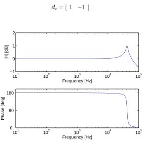
In order to implement Direct Velocity Feedback (DVFB) in the control loop, an integrator is used which provides the velocity as the error signal to the controller. With time harmonic excitation, the integration can be expressed by the reciprocal ofjω, so that the accelerometer with integrator provides the following control voltage ˆva:

ˆ

va=

cσ

jω(wc−wa). (3.57)

Eq.(3.57) can be grouped into the following matrix form:

ˆ

va =

cσ

jωdcw

= ₋cσ

ω2dcw˙, (3.58)

where w˙ is a 2-element column vector with the velocity of the plate at the control position ˙

wc and that of the inertia mass in the accelerometer sensor ˙wa:

˙

w=

(

˙

wc

˙

wa

)

(39)

dc is a 2-element row vector given below:

dc = [ 1 −1 ]. (3.60)

101 102 103 104 105

−1 0 1 2

[image:39.612.157.439.71.350.2]

Frequency [Hz]

|H| [dB]

101 102 103 104 105

0 90 180

Frequency [Hz]

Phase [deg]

Figure 3.11: Transfer function between the acceleration of the panel at the sensor position and the voltage signal output of the accelerometer

3.4.2 Fully coupled model

In this section the open loop FRF is derived by taking into account the response of an accelerometer sensor modeled as a suspended mass with spring and dashpot. In this case, the velocity at sensor location ˙wc is given by the following matrix expression:

˙

wc =Ycpfp+Ycmfm+YcMMt+Ycc(fa1 +fh), (3.61)

where Ycc is the mobility function between the collocated point force and the velocity at

the control position, where the accelerometer is fixed. fh represents the inertia effect of

the housing mass of the accelerometer, and fa1 is the reaction force of the seismic mass of

the accelerometer, transmitted via the elastic piezoelectric elements. fh and fa1 are simply

modeled as a single lumped mass acting at (xc, yc). Figure 3.12 illustrates details regarding

the displacement and forces acting on the elements of the accelerometer, which is mounted on the plate at the center of the piezoelectric patch actuator. Since the displacement of housing mass is corresponding to that of the plate, the force generated by inertia effect of the housing mass fh is given as:

fh =−jωmhw˙c. (3.62)

(40)

A

fh

ma

mh

ka ca

fs1

-f_s1 fs2

-fs2

Figure 3.12: Schematic representation of a piezoelectric accelerometer transducer, and the notation of the forces and displacement at the connecting points between the elements of the accelerometer and the smart panel

function of the angular velocity along the edges of the patch in correspondence to the spring elementsθ˙.

When the dynamics effect of the sensor is taken into account, the vectors of the elemental velocities ˙we and the angular velocities ˙θ are given by:

˙

wm = Ympfp+Ymmf_m+YmMMt+Ymc(fa1+fh), (3.63) ˙

θ = Yθpfp +Yθmfm+YθMMt+Yθc(fa1+fh), (3.64)

whereYmcis an2m-element column vector with the mobility functions between the point force

on the plate generated by the dynamics effect of the accelerometer acting at the sensing point and the velocities at the center of the actuator mass elements. Yθc is a 4nk-element column

vector with the mobility functions between the point force generated by the dynamics effect of the accelerometer acting at the sensing point and the angular velocities along the edges of the patch in correspondence to the actuator springs. Details regarding the mobility functions

Ymc and Yθc are given in section 5 of Appendix B. After some algebraic manipulations,

the velocity of the plate at sensor’s position ˙wc can be written as a function of the primary

excitation fp, reaction force of the accelerometer sensor fa1 and the control moment Mc:

˙

wc = ˜Ycpfp+YfcMMc+ ˜Yccfa1. (3.65)

where ˜Ycp, YecM and ˜Ycc are given in Appendix B.

The reaction force of the accelerometer fa1 is identical to the force applied on the inertia

mass fa2 with opposite sign:

fa1 =−fa2. (3.66)

The force applied to the inertia massfa2 was already given in Eq.(3.48):

fa2 = maw¨a

= ca( ˙wc−w˙a) +

ka

jω( ˙wc−w˙a) (3.67)

= ca+

ka

jω !

(41)

The velocity of the seismic mass ˙wa is given using the mobility term:

˙

wa =

1

jωma

fa2 =Yaafa2. (3.68)

Eq.(3.65) and Eq.(3.68) can be grouped in a matrix form as follows:

(

˙

wc

˙

wa

)

=w˙ =Yafa+Ypfp+YMMc, (3.69)

where the 2 _× 2 matrix Ya, the 2-element column vector Yp, and the 2 ×4nk matrix YM

are given as follows:

Ya =

"

˜

Ycc 0

0 Yaa

#

(3.70)

Yp =

"

˜

Ycp

0

#

(3.71)

YM =

" f

YcM

0

#

, (3.72)

and f_a is a 2-element column vector that consists of the forces acting on the seismic mass and base mass:

f_a=

" fa1

fa2

#

. (3.73)

Using Eq.(3.66) and Eq.(3.67), the force vector f_a is derived in terms of the following impedance relation:

f_a=Zaw˙, (3.74)

where the impedance matrixZa is given as:

Za= " _k_a

jω +ca −

ka

jω −ca

−ka

jω−ca ka

jω +ca

#

. (3.75)

Substituting Eq.(3.74) into Eq.(3.69), and solving the equation with respect tow˙ leads to the following result:

˙

w = [I +YaZa]

−₁

(Ypfp+YMMc)

= Y˜pfp+Y˜MMc, (3.76)

whereI denote a 2 _×2 identity matrix, and Y˜p and Y˜M are given by:

˜

Yp = [I+YaZa]

−₁

Yp (3.77)

˜

YM = [I+YaZa]

−₁

YM (3.78)

Substituting Eq.(3.76) and Eq.(3.38)into Eq.(3.58), the open loop sensor-actuator FRF

Gc between the integrated output signal voltage from the accelerometer sensor ˆva and the

input signal voltage to the piezoelectric actuator Vc is given as:

Gc =

ˆ

va

Vc

=₋cα

nk

cσ

(42)

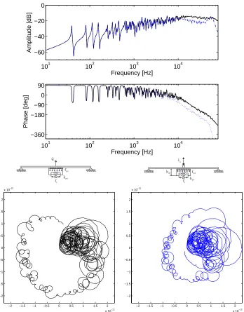
Figure 3.13 shows the Bode plot of the open loop sensor-actuator FRF using the actuator-plate (solid line) and actuator-actuator-plate-sensor (dotted line) fully coupled models. At low fre-quencies, below about 8kHz, the sensor-actuator FRF derived with the actuator-plate-sensor fully coupled model is very similar to that of the actuator-plate model. In fact, up to 3kHz, the FRFs are characterized by an alternating sequence of resonances and anti-resonances, so that the phase is constrained between 90deg. Above 3kHz the modal density of the plate is so high that the FRFs are characterized by a smoother curve. The mean value of the FRF tends to raise with the frequency. This is a typical feature of strain actuators, which is due to the fact that the piezoelectric patch generates bending moments on the plate along the four edges of the patch itself and thus better excites the plate as the flexural wavelength approaches or becomes smaller than the size of the actuator, i.e. at higher frequencies. The FRFs are also characterised by a constant phase lag, which is due to the non perfect collocation between the position of the error signal detection at the centre of the piezoelectric patch and the bending control excitation at the edges of the piezoelectric patch [15].

[image:42.612.176.417.389.491.2]

At high frequencies, above 10kHz, the FRF of the actuator-plate-sensor coupled model is characterized by a constant amplitude roll off and additional phase lag followed by a wide frequency band peak with a 180deg phase lag. The amplitude roll off is due to the mass effect introduced by the accelerometer. Also, the extra peak and 180deg phase lag are caused by the resonance of the accelerometer which, according to the given parameter of the sensor considered here, has been calculated at about 50kHz. The simulated FRF shows this resonance peak at 54.8kHz due to the fully coupled response of the plate and accelerometer sensor.

Table 3.1: Geometric and physical properties of the accelerometer

Parameter value

Total mass mta = 2.0 [g]

Inertia mass ma = 0.6(0.7) [g]

Stiffness ka = 59.22 ×106 [N/m]

Viscous damping ζa = 0.05

Damping ca = 18.85 [Nsec/m]

Strain transducers for active control lumped parameter model

SCIENTIFIC PUBLICATIONS BY THE ISVR

Contents

List of Figures

List of Tables

Chapter 1

INTRODUCTION

1.1

Active Structural Acoustic Control

1.2

Scope and Objectives

1.3

Structure of the Report

Chapter 2

ACTIVE CONTROL AND

STABILITY

2.1

DVFB Control

V

-H

S

+

+

Y

f

w

G

2.2

Open Loop Frequency Response Function

2.3

Control Performance

Chapter 3

MODEL PROBLEM

3.1

Actuator Mass Effect

m

f

3.2

Actuator Stiffness Effect

3.3

Actuator-Panel Fully Coupled Model

3.4

Sensor-Actuator Fully Coupled Model

3.4.1

Sensor dynamics

v

+

k

c

m

m

S

-w

w

3.4.2

Fully coupled model

_c