On model selection in data envelopment analysis: a multivariate statistical approach

Discussion Papers in

Management

On Model Selection in Data Envelopment Analysis: A

Multivariate Statistical Approach

C. Serrano Cinca

Department of Accounting and Finance

University of Zaragoza, Spain

C. Mar Molinero

School of Management

University of Southampton

F. Chaparro García

Department of Accounting

Universidad Autónoma de Bucaramanga, Colombia

Number M02-7

ON MODEL SELECTION IN DATA ENVELOPMENT ANALYSIS: A

MULTIVARIATE STATISTICAL APPROACH

By:

C. Serrano Cinca

Department of Accounting and Finance University of Zaragoza, Spain.

http://ciberconta.unizar.es/charles.htm

[email protected]

C. Mar Molinero

Department of Management University of Southampton, UK. [email protected]

F. Chaparro García

Department of Accounting

Universidad Autónoma de Bucaramanga, Colombia [email protected]

This version: May 2002

ON MODEL SELECTION IN DATA ENVELOPMENT ANALYSIS: A

MULTIVARIATE STATISTICAL APPROACH

ABSTRACT

This paper addresses an important issue in DEA: the selection of inputs and outputs to be included in a model. A two-stage methodology is suggested. The first stage applies a methodology based on comparing reduced models that do not include a particular input/output with extended models that include it. The second stage uses the tools of multivariate statistical analysis to visualize important aspects of the models considered. In this way model selection combines mathematical tools, statistical analysis, and the exercise of judgment. The methodology has the advantage of explaining why some Decision Making Units (DMUs) appear to be efficient under some models and inefficient under other models. It is also possible to produce rankings of DMUs that are a consensus over all the models. The methodology is illustrated with the help of a case study: the efficiency of Spanish banks. It is found that, in this case, there are various defensible definitions of efficiency, and it is suggested that a variety of models should be estimated.

KEY WORDS

ON MODEL SELECTION IN DATA ENVELOPMENT ANALYSIS: A

MULTIVARIATE STATISTICAL APPROACH

1. INTRODUCTION

Data Envelopment Analysis (DEA) is becoming widely used to assess the efficiency of organizations with multiple homogeneous decision units that produce several outputs with a variety of inputs. Examples are universities, hospitals, and banks. For an extensive bibliography see Emrouznejad and Thanassoulis (1996). The advantages of DEA, as a non-parametric approach that uses multiple comparisons to identify best practice, are now clear. But there still remain many difficult problems that are not totally resolved in practice. This paper addresses one of them: how to decide which inputs and which outputs to include.

The identification of the inputs and outputs that need to be included in a particular application of DEA presents a variety of problems. Different authors that approach modeling in a given context may choose different sets of inputs and outputs. An example is the study of the efficiency of banking institutions, which will be discussed below. A way out is to include all possible inputs and outputs in the model, but this is not devoid of problems. First, the more inputs and outputs are included in the model, the more data is needed to obtain reliable results; see Pedraja et al (1999). Second, DMUs that use extreme values of inputs or outputs may become 100% efficient. By extreme values we mean the lowest value of an input and the highest value of an output. Clearly, the more inputs and outputs are included in the model, the more units will be efficient. Taking a metaphor from a different context, we would find that the “naughty boy” who puts the least effort in the class and gains low marks would be efficient under a DEA model that includes amount of effort as an input. But if many inputs and outputs are included, some of them may be highly correlated and, therefore, redundant. On the other hand, removing inputs or outputs from a model will decrease efficiency estimates, which will, at best remain constant. This decrease would affect some DMUs more than others.

the analyst’s judgment as well as on the data provided? It is clear that a structured approach to input/output selection is both complex and important; see Kittelsen (1993), Parkin and Hollingsworth (1997).

Several methods have been proposed for input/output selection. A possible approach is to use Principal Components Analysis (PCA) as a data reduction tool to select a number of inputs and outputs that are representative of the data available, but the fact that a variable is uncorrelated with others does not mean that is relevant in the modeling of efficiency. The converse is also true: two variables may be correlated but they may both be needed in the modeling of efficiency. Adler and Golany (2001) go as far as working directly with the principal components. This has the advantage that there is no information loss but, apart from the problems that calculating and interpreting the components creates, is little different from using PCA to select a reduced set of outputs and inputs. Norman and Stoker (1991) propose a step-wise approach: they start with a simple model, calculate efficiencies for all DMUs, and correlate such efficiencies with the values of excluded variables; any variable that produces a sufficiently high value of Pearson’s correlation coefficient is included in the specification and the model is re-estimated. This approach has the disadvantage that correlations may not be affected by changes in efficiencies; for example, if the inclusion of a variable results in a proportional increase of the efficiencies of all DMUs, the correlation coefficient does not change.

A transparent method for input/output selection in DEA was suggested by Serrano Cinca and Mar Molinero (2001), we will refer to this method as SM. This method is not sequential in the sense that efficiencies are estimated for each DMU under all possible input/output combinations. This results in a matrix of models by specification that is visualized using multivariate statistical techniques: PCA and Cluster Analysis. Visualization reveals the way in which the different specifications are related, and the reasons why they are related. Model selection can then benefit from the combination of both a strong statistical basis and the exercise of judgment, but this time exercise of judgment does not mean imposing preconceptions on the model. There are further advantages, in that the reasons why a particular DMU is, or fails to be, efficient under a given model also becomes clear. It is possible for two DMUs to achieve the same efficiency score under a given model, but for different reasons; these reasons also become apparent. Furthermore, since given any two input/output combinations, the correlation between efficiencies is clearly positive, it follows that the first principal component is a measure of size. Thus, the score of a given DMU on the first principal component can be interpreted as an overall measure of efficiency under all possible specifications, and DMU rankings can be produced. This method works well with a small number of inputs and outputs, perhaps 2 or 3 of each, but if the total number of inputs plus outputs increases, the number of possible combinations also increases and its direct application becomes problematic.

This paper attempts to combine the RPS method with the SM method in order to enjoy the benefits that they both bring without having to suffer from their disadvantages. The RPS systematic exploration of possible specifications is followed first, and the results are interpreted using the SM visualization. The procedure is applied to a classical DEA problem: the study of the efficiency of financial institutions, in particular to a data set of 55 Spanish banks. For a review of efficiency issues in financial institutions see Berger and Humphrey (1997). For a review of the Spanish banking context see Grifell-Tatje and Lovell (1997), Dietsch and Lozano-Vivas (2000).

2. EFICIENCY IN FINANCIAL INSTITUTIONS

The issue of which inputs and which outputs should be included in a DEA models has been much debated in financial sector applications. It is clear from the review of DEA applications in this area by Berger and Humphrey (1997) that most studies start with a debate on input/output selection. Different authors, when working on the same problem, often use different input/output sets; a given input or output is sometimes included and sometimes excluded from a DEA study; and there is even the case that a variable (deposits) is included both in the input and in the output set. One ends up with the feeling that it is unclear what is meant by efficiency in financial institutions. The matter is further complicated by the fact that it is possible to make a particular financial DMU either efficient or inefficient just by adding or removing variables from the data set. This is, of course, not specific to financial efficiency modeling.

It is usual to make a distinction between the intermediation approach and the production approach in efficiency studies of financial institutions ; Athanassopoulos (1997). Under the production approach, banks perform a set of tasks such as: issue loans, collect deposits, produce credit reports, and so on. These are the outputs. Typical inputs are staff and plant. Under the intermediation approach, financial institutions are intermediaries in financial flows: they collect deposits (inputs) and issue loans (inputs) in order to make a profit (output). Neither approach is totally satisfactory, as both capture partial aspects of the way in which a bank operates; see Berger and Humphrey (1997). There is a view, reported by Oral and Yolalan (1990) that no single model should be entertained, but that decision makers should be confronted with a variety of models. In their own words: “having considered different input-output combinations, the managers of The Bank felt more comfortable with the way the study was conducted and had more confidence in the results”. But even in this case, there is still a model selection problem, since it has to be decided which input/output combinations should be made explicit to management.

Input A: Number of employees

Input B: Fixed assets

Input C: Deposits

Input D: Operating expenses

Output 1: Operating Income

Output 2: Deposits

Output 3: Loans

Output 4: Securities

A further modeling issue is whether the DEA model should include Constant Returns to Scale (CRS) or Variable Returns to Scale (VRS).

The particular inputs, outputs, and returns to scale combinations included in a particular model will be highlighted in an obvious way by simply referring to the model in terms of the letters associated with inputs, the numbers associated with outputs, and v or c depending on whether VRS or CRS apply. For example, A23v would refer to a model with a single input- number of employees (A)-, two outputs- deposits (2) and loans (3)-, which is estimated under variable returns to scale (v). This would correspond to a view of the world in which banks, operating under variable returns to scale, have employees whose tasks are to collect deposits and to issue loans. Note that deposits have been included both as an input and as an output, as they tend to be treated as inputs in the intermediation approach and as an output in the production approach. In order to avoid confusion, no combinations that treat deposits both as inputs and as outputs will be estimated.

3. A CASE STUDY: THE EFFICIENCY OF SPANISH BANKS

obtained from the 2001 Statistical Yearbook of the Higher Banking Council (Consejo Superior Bancario). The data set has been reproduced in Table 1.

Table 1 about here

The number of input/output combinations with four inputs and four outputs can be calculated. In general, with n inputs and m outputs the number of combinations is given by the formula:

?

?

1

C

*

C

? ?

n! n

i Ci_n

? ? ? ? ? ? ? ? ? ? ?

In the particular case where n=4 and m=4.

?

? ?

?

4 3 4 2 4 1 4 4 4 3 4 2 4 1 4 4 1 4 4

1

C

*

?

C

?

C

?

C

?

C

?

C

*

C

?

C

?

C

?

C

?

i i

i

= 225

Since each input/output combination can be estimated under VRS or CRS, the total number of possible combinations is 450. The need to limit the search is clear. It is for this reason that the specification search will start with the RPS approach. The results will then be made explicit using the SM visualization and, in the final subsection interpreted by means of Cluster Analysis and Property Fitting, a regression-based approach.

3.1 DEA EFFICIENCY CALCULATION

this procedure. It is concluded that, at least for the moment, models should be estimated under VRS.

Table 2 about here

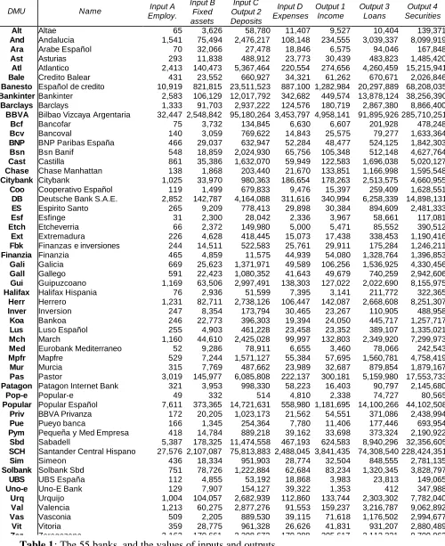
This initial model is next augmented with an extra input or an extra output. Adding an input or an output means that efficiencies can increase but cannot decrease. The percentage of DMUs whose efficiency increases by more than 10% is noted. This is done in sequence with the models AB1v, AC1v, AD1v, A12v, A13v, and A14v. The largest changes are obtained with model A14v (65.5%) which becomes the model to be extended in step 2.

In step 2, the model A14v is simplified from VRS to CRS, and it is found that the efficiencies of 29.1% of the DMUs decline in more than 10%. This decline is considered to be too large, and the VRS specification is retained. Next, the model A14v is augmented with inputs and outputs, one at a time, and the changes noted. The models so considered are: A124v, A134v, AB14v, AC14v, and AD14v. When model AC14v is estimated, it is found that 50.9% of DMUs increase their efficiency by more than 10%. Therefore, this model is now kept as the basis for comparisons.

Finally, in step 3, only reductions in inputs and outputs are considered, something that results in declines in efficiency. If removing an input (output) does not affect efficiencies, it is not necessary to keep that input (output). In this step only models C14v and AC4v are contemplated. The model finally chosen is AC4v. Of course, the search could have been extended: more extensions could have been contemplated, and more simplifications entertained, but there is a moment when a decision has to be taken that the model is satisfactory enough on the basis of more than simple statistical performance. In the process of conducting this search 16 models were estimated. The process described above is summarized in Table 2.

Table 3 about here

Simple visual inspection of the data in Table 3 is illuminating. Chase is the only bank that appears 100% efficient under all 16 models. It is more common for banks to appear as 100% efficient under some models but not to achieve full efficiency under other models. This is the case of BBVA, Bankinter, Priv, Coo, Esf, Finanzia, Mpfr, Popular, Pop-e, SCH, and Vas. Some banks obtain low efficiency scores under all models; examples are BNP, Inver, and UBS.

It is also noticeable the case of banks that achieve the same efficiency score under some models but very different scores under other models. For example, Pop-e, an on-line bank, and Coo are both 100% efficient under AC4v, AC14v, and AB14v, but achieve very different scores under other models. Pop-e is 100% efficient under AB1v, AC1v, and C14v, while Coo only achieves 47%, 34%, and 12% on the same models. Coo is 100% efficient under A12v, A14v, A124v, A134v, and AD14v, while Pop-e achieves 63%, 63%, 63%, 66%, and 63% under the same models. The cases of Pop-e and Coo will be further discussed below.

In conclusion, from the fact that a financial institution achieves different scores under different models we deduce that the way in which the model is defined matters. Furthermore, the fact that some institutions obtain the same score under some models and very different scores under other models suggests that there is no single path to efficiency, and that we ought to investigate what lies behind the efficiency score. Institutions may have strong points that are captured by some models, and stand out for the efficient use of an input or an output. It is also be possible that some institutions owe their efficiency values to extreme values of inputs or outputs, and that they are mavericks or self-comparators.

Interesting as they are the insights obtained by mere visual inspection, it is desirable to apply formal multivariate methods to the analysis of Table 3. In this paper we will show how to reveal its main features using PCA, Hierarchical Cluster Analysis (HCA), and Property Fitting (Pro-Fit).

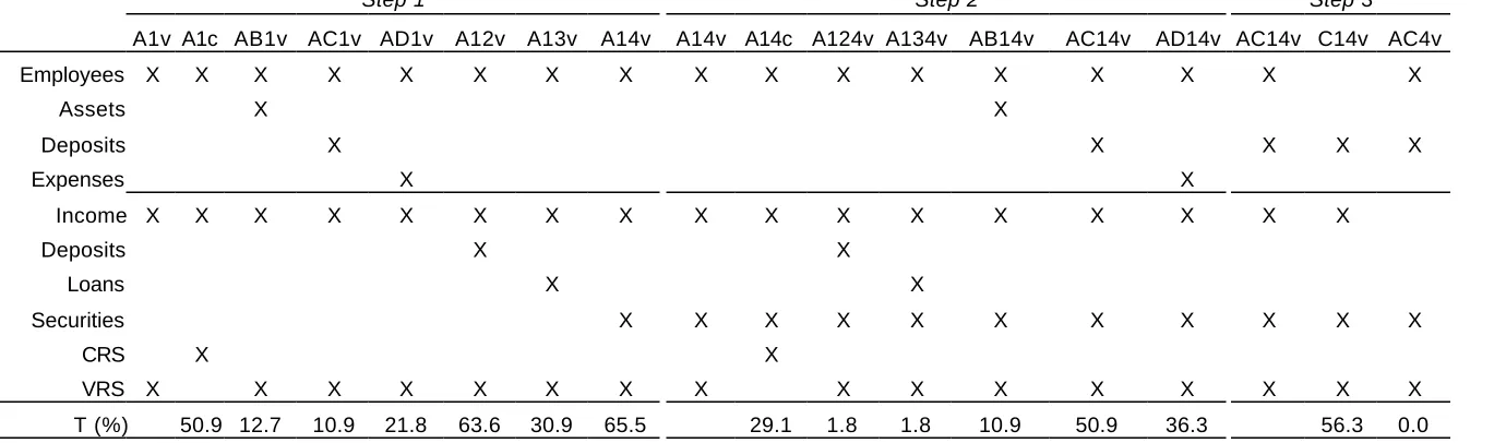
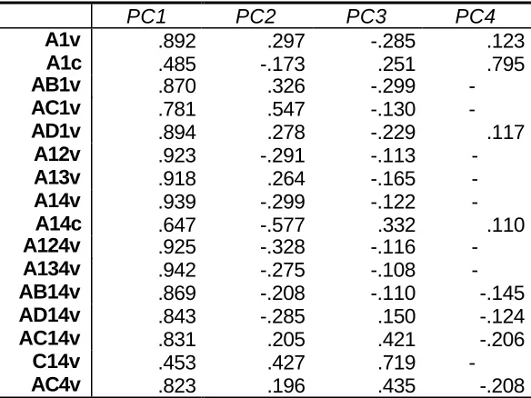
Efficiency values shown in Table 3 have been treated as observations in a matrix where variables are the 16 models and cases are the 55 banks. PCA has been performed on this data set. The limit for eigenvalue extraction was set on 0.8 in line with Joliffe’s (1972) recommendation that setting the limit to 1 may throw away too much information. Four components were found to be associated with eigenvalues greater than 0.8. The first principal component accounts for 68.6% of the total variability in the data, a very large proportion but not a surprisingly large amount since the correlations between the 16 variables are positive, which is a consequence of the fact that all the variables are different measures of efficiency; see Chatfield and Collins (1980). This component can clearly be interpreted as an overall measure of efficiency. The second component accounts for only 10.9% of the variability; the third accounts for 8.8%; and the fourth for 5.1%. These results are summarized in Table 4.

Table 4 about here

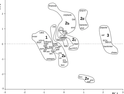
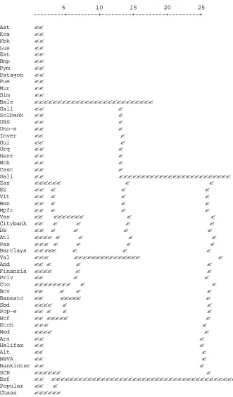
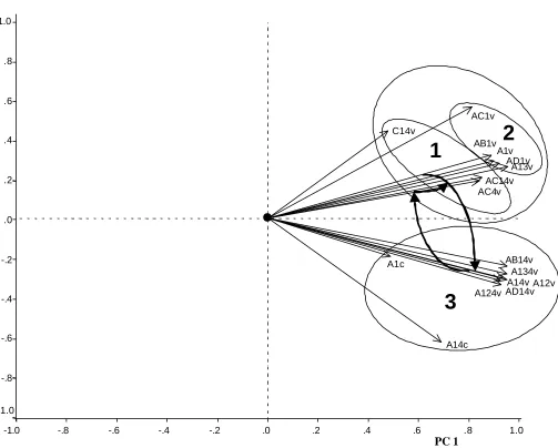
Component scores were calculated for each bank. Figure 1 shows the scores for the first two principal components. The position of each bank on the component space could be interpreted by visual inspection, but before so doing the figure was completed with the superimposition of the results of Hierarchical Cluster Analysis (HCA). To perform HCA Euclidean distances were calculated between pairs of banks in Table 3. These Euclidean distances were used as input in Ward’s method, which maximizes compactness. The dendrogram can be seen in Figure 2.

Figure 1 about here

Figure 2 about here

An examination of the dendrogram shows that banks neatly divide into three clusters. The second cluster can be subdivided into five subclusters. The outlines of the clusters and subclusters have been drawn in Figure 1.

component and, as expected, achieve full efficiency under most models. BBVA and SCH are the two leading banks in Spanish banking, and are amongst the European banks with the highest market value. The Popular Bank is often described as the best managed bank in Europe by specialized magazines such as, for example, The Banker. Bankinter is a middle-sized bank that leads Internet banking in Spain, collecting 25% of on-line deposits. Chase Manhattan is one of the few international banks that has been able to penetrate the very competitive Spanish banking system. The presence of Esf amongst the group of “the great and the good” is puzzling. When Table 1 is examined it is found that Esf has the smallest number of employees in the data set, just 31 as opposed to BBVA that has 32447. One would expect models that contain employees as an input to reveal this bank as 100% efficient. This is indeed what is found: Esf achieves only 3% efficiency in model C14v, which does not include employees as an input. We could conjecture that Esf is the “naughty boy” in the class.

Cluster 1, which groups banks associated with low efficiency scores, contains, amongst others, Inver, BNP, UBS, and Uno-e. This cluster is situated on the left hand side of Figure 1, in the region associated with high negative scores in the first principal component.

The various subgroups that make up Cluster 2 are situated between Cluster 1 and Cluster 3 in Figure 1. Cluster 2d (Pop-e, Banesto, SBD) is located near the cluster that groups efficient banks, on the right hand side of Figure 1, and towards the top of this figure. To the left of Cluster 2d, but also on the top of the figure, is Cluster 2b, which includes institutions such as Citybank. On the same vertical as Cluster 2d, but towards the bottom of Figure 1, one finds Cluster 2e, which contains Priv, Coo, and Bcv. This last cluster is clearly distinct from all the others on the representation, suggesting anomalous or maverick behavior.

There is little ambiguity as to the meaning of the first principal component, and the position of a bank along this component has been clearly seen to be associated with efficiency, but no meaning has yet been attached to the remaining principal components. In particular, in order to completely interpret Figure 1 it is necessary to attach meaning to the second principal component.

reason, they will be positively correlated, something that results in a large first principal component which measures an overall effect; see Dunteman (1989) for a discussion. The highest loadings on PC1 are associated with A134v, A14v, A124v, A12v, and A13v.

The loadings associated with PC2 sometimes take positive values and sometimes take negative values, as was to be expected. The models that contain C (deposits as an input) are associated with high positive component loadings in PC2. Deposits as an input are a characteristic of the intermediation approach to modeling efficiency. It is, therefore, to be expected that the second principal component will discriminate between intermediation and production approaches to modeling efficiency. This issue will be further explored below.

The relationships that exist between models and principal components will be next explored in a more formal way by means of Property Fitting, a regression-based approach, and by means of HCA.

Table 5 about here

3.3 RESULTS INTERPRETATION: PROFIT AND CLUSTER ANALYSIS.

Figure 1 has been obtained from the efficiencies achieved under the various models considered applying the RPS methodology. In this subsection, two techniques are used to further interpret the relationships between the different models; to see how models and components are related; and to explore in what sense the different models capture different aspects of efficiency.

there could be an association between the position of a bank in the space of the principal components and the levels of efficiency obtained. But the location of the bank in the space spanned by the principal components is given by its component scores. Hence, we consider the possibility of a relationship between component scores and efficiency under a given model. In formal terms we can write:

?

?

k k k k k m

k f PC PC PC PC e

E ? 1 , 2 , 3 , 4 ?

where E_kmis the efficiency obtained by bank k under model m; PC1 is the value of_k

the first component score for bank k; PC2 is the value of the second component score for_k bank k, and so on. m

k

e is an error term.

In the absence of any other information, we assume function f to be linear.

m k k k

k k

m

k PC PC PC PC e

E ? ?₀ ? ?₁ 1 ? ?₂ 2 ??₃ 3 ? ?₄ 4 ?

This is just a regression equation where the ?i are the unknowns. It can be estimated using any regression routine and the results drawn in the form of a vector through Figure 1. This vector will point in the direction where efficiencies increase. The representation of the results obtained from model A1v can be seen in Figure 3. It is apparent that, in the direction of this vector, banks are ordered from lowest to highest efficiency under A1v. A full description of Pro-Fit can be found in Schiffman et al (1981). This same procedure has been followed with all 16 models, and all of them have been represented in Figure 3.

Figure 3 about here

Table 6 about here

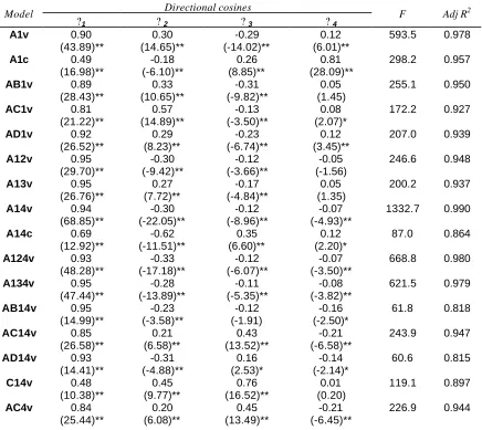
It can be seen in Table 6 that R2 values are very high: always above 0.8. The same thing can be said about F statistics, which always exceed the critical value.

The Pro-Fit lines associated with all the models have been represented in Figure 3 on the component score space spanned by PC1 and PC2. Pro-Fit lines are the wind’s rose that helps to steer through Figure 1 in the search for efficiency.

All the 16 vectors point towards the right hand side forming a fan. In the center of the fan is PC1, which is consistent with PC1 being an overall measure of efficiency under all the models. There has been much debate on how to rank DMUs; Andersen and Petersen (1993), Doyle and Green (1994), Sinuany-Stern and Friedman (1998), Raveh (2000). Here we see a natural way of creating such a ranking: the ordering in terms of the score of the first principal component under a variety of model specifications.

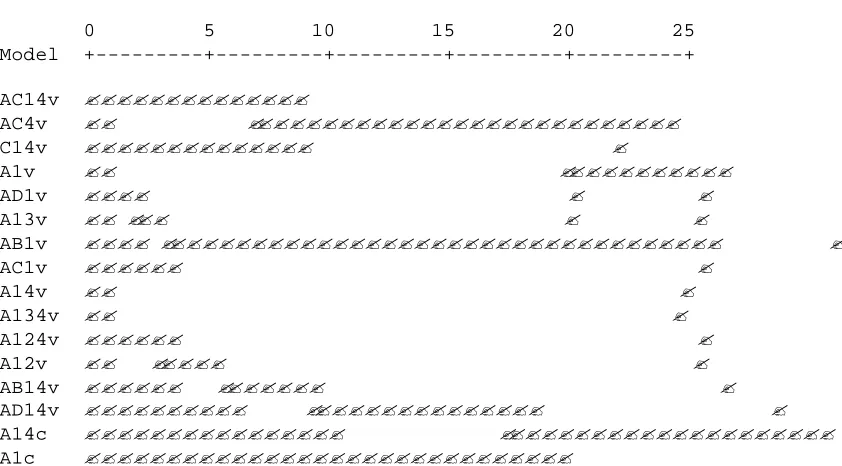
Had a vector coincided with the first principal component, its associated model could have been taken to be a consensus view of efficiency in banking. However, no directional vector coincides with the first principal component. PC1 appears to divide the fan in at least two sheaves of vectors, some pointing towards the top of the figure and some pointing towards the bottom of the figure. It is interesting to notice that models with C in their definition (deposits as an input), always point towards the top of the figure, confirming that there are at least two different definitions of efficiency in banking: two paradigms. But we are working with projections of a five dimensional representation on the first two coordinates, to be sure that what we observe in PC1 and PC2 represents reality, we have performed a second HCA. To perform this HCA we start from the data in Table 3. Euclidean distances have been calculated between models using banks as observations, and Ward’s clustering procedure was applied. The resulting dendrogram is reproduced in Figure 4.

Figure 4 about here

Cluster 1 contains 3 models: AC14v, AC4v, and C14v. The vectors associated with them point towards the top of Figure 3. All of them contain the input C; i.e., they all contain deposits as an input, a characteristic of the intermediation approach. Cluster 2 contains five models: AC1v, AB1v, A1v, AD1v, and A13v. Their associated vectors point towards the top. Finally, Cluster 3 contains the remaining eight models whose associated vectors point towards the bottom of the figure. The relevance of variable returns to scale is highlighted by the fact that vectors A14c and A1c appear to be distinct from the rest both in Figure 3 and in the dendrogram.

The way in which the RPS method proceeds in the search for the “best” model is now clear in Figure 3. The starting point was model A1v, in Cluster 2. Amongst all the models that augment this basic model (see Table 2), it selects A14v, the most distant one in Figure 3, a member of cluster 3. In the next step, it selects again the most distant model amongst all those that are contemplated, AC14v, a model that belongs to Cluster 1. Finally, in the last step, it chooses the most similar model to AC14v containing one less input or output if such a model exists. Since models that are similar to be one being considered are those whose associated vectors are close to the vector associated with AC14v in Figure 3, the selected model, AC4v, also belongs to cluster 1. The path followed by this specification search has been highlighted in bold in Figure 3.

It has already been discussed that there are at least two paradigms in what represents efficiency in banking. What the RPS methodology appears to be doing is to jump from a paradigm to a different one without stopping to think whether, on grounds other than model selection procedures, one paradigm is to be preferred to other alternatives. But, why should a paradigm be preferred to an alternative one? The decision to implement a particular paradigm should be based on a view of the world and not on a set of mathematical rules.

In view of what has been observed in Figures 1 and 3, the following considerations are in line.

ii) If models group into several clusters, one should consider entertaining a variety of models, one from each cluster. This would acknowledge the fact that no single definition of efficiency exists. This is the situation faced in the present case study. For example, in the case of Spanish banks such models could be AC4v, A1v, and A14v. These models have been chosen taking into account that they are parsimonious and representative of the models in their clusters. Of course, dealing with a variety of definitions of efficiency means dealing with a multicriteria situation.

Knowing whether we are in case i) or in case ii) requires having a clear view of the relationship that exists between models. This is why visualization is important.

4 CONCLUSIONS

It has been argued that choosing an appropriate set of inputs and outputs to be included in a DEA model is both problematic and important. Model selection procedures based on data reduction may miss important inputs or outputs that should be included in a model. Methods that are based on comparison of efficiencies using correlation procedures may produce misleading results. Just adding extra inputs or extra outputs may throw as efficient cases that are just extreme values.

Two model selection procedures were identified as satisfactory, one due to Ruiz, Pastor, and Sirvent (2002), which is based on comparing a reduced and an augmented model, and one due to Serrano Cinca and Mar Molinero (2001), which visualizes the relationships between models. Unfortunately, the first approach suffers from being mechanistic and relatively obscure, while the second one may generate too many models for consideration. A hybrid of the two approaches has been demonstrated to be sound and to be revealing enough to throw light on the main features of the situation at hand.

A case study, banks in Spain, has been used to demonstrate how the procedure works. There has been much debate on how to measure efficiency in financial institutions. The proposed method has visualized the various definitions of efficiency, and has shown that, in this case there is no holy grail to be found. There is no such thing as “the best model”. Efficiency in a bank is a multicriteria concept, and either should be studied in a variety of ways or a decision must be made on what is the appropriate benchmark for a given bank. The procedure proposed here has made the choice explicit.

The suggested methodology has further advantages. DMUs can be ranked in an unambiguous way under a variety of specifications. It is possible to explain why two DMUs achieve different efficiencies under a given model. Finally, even when two DMUs achieve the same level of efficiency, it is possible to explain in which way they differ, when they do, and, by so doing, their strong points can be identified.

Adler, N. and Golany, B. (2001): Evaluation of deregulated airline networks using data envelopment analysis combined with principal components analysis with an application to Western Europe. European Journal of Operational Research, 132, 260-273.

Andersen P,. and Petersen N.C. (1993): A procedure for ranking efficient units in data envelopment analysis. Management Science, 39, 1261-1264.

Athanassopoulos, A.D. (1997): Service quality and operating efficiency synergies for management control in the provision of financial services: Evidence from Greek bank branches, European Journal of Operational Research, 98 (2), 300-313

Berger, A.N., and Humphrey, D.B., (1997): Efficiency of financial institutions: International survey and directions for future research. European Journal of Operational Research, 98 (2), 175-212.

Chatfield, C. and Collins, A.J. (1980): Introduction to Multivariate Analysis. Chapman and Hall, London.

Dietsch, M. and Lozano-Vivas, A. (2000): How the environment determines banking efficiency: a comparison between French and Spanish industries. Journal of Banking and Finance, 24, 985-1004.

Doyle, J., and Green, R. (1994): Efficiency and cross-efficiency in DEA: derivations, meanings and uses. Journal of the Operational Research Society, 45, 567-578.

Dunteman G.H. (1989): Principal Component Analysis. Sage Publications Ltd. London, UK. Emrouznejad, A. and Thanassoulis, E. (1996): An extensive bibliography of Data Envelopment

Analysis. Journal Papers. Working paper. Warwick Business School.

Grifell-Tatje, E and Lovell, C.A.K. (1997): The sources of productivity change in Spanish banking. European Journal of Operational Research, 98, 364-380.

Joliffe, I.T. (1972): Discarding variables in Principal Components Analysis. Applied Statistics, 21, 160-173.

Kittelsen, S. A. C. (1993): "Stepwise DEA; Choosing Variables for Measuring Technical Efficiency in Norwegian Electricity Distribution", Memorandum No. 6/1993, Department of Economics, University of Oslo.

Lovell, C.A.K, and Pastor, J.T (1997): Target setting: an application to a bank branch network. European Journal of Operational Research, 98, 290-299.

Mancebon, M.J. and Mar Molinero, C. (2000): Performance in primary schools. Journal of the Operational Research Society, 51, 843-854.

Parkin, D. and Hollingsworth, B. (1997): Measuring production efficiency of acute hospitals in Scotland, 1991-94: validity issues in Data Envelopment Analysis.

Pedraja, F.; Salinas, J; Smith, P. (1999): On the quality of the Data Envelopment Analysis model. Journal of the Operational Research Society, 50, 636-645.

Raveh, A. (2000): The Greek banking system: reanalysis of performance. European Journal of Operational Research, 120, 525-534.

Ruiz J.L.; Pastor, J.; Sirvent, I. (2002): A statistical test for radial DEA models. Operations Research, forthcoming.

Serrano Cinca, C. and Mar Molinero, M. (2001): Selecting DEA specifications and ranking units via PCA, Discussion Papers in Management, M01-3, University of Southampton.

Schiffman, J.F., Reynolds, M.L. and Young, F.W. (1981): Introduction to Multidimensional Scaling: Theory, Methods and Applications. Academic Press, London.

Table 1: The 55 banks, and the values of inputs and outputs.

DMU Name Input A Employ. Input B Fixed assets Input C Output 2 Deposits Input D Expenses Output 1 Income Output 3 Loans Output 4 Securities

Alt Altae 65 3,626 58,780 11,407 9,527 10,404 139,371

And Andalucia 1,541 75,494 2,476,217 108,148 234,555 3,039,337 8,099,919

Ara Arabe Español 70 32,066 27,478 18,846 6,575 94,046 167,848

Ast Asturias 293 11,838 488,912 23,773 30,439 483,823 1,485,420

Atl Atlantico 2,413 140,473 5,367,464 220,554 274,656 4,260,459 15,215,941

Bale Credito Balear 431 23,552 660,927 34,321 61,262 670,671 2,026,846

Banesto Español de credito 10,919 821,815 23,511,523 887,100 1,282,984 20,297,889 68,208,035

Bankinter Bankinter 2,583 106,129 12,017,792 342,682 449,574 13,878,124 38,256,390

Barclays Barclays 1,333 91,703 2,937,222 124,576 180,719 2,867,380 8,866,400

BBVA Bilbao Vizcaya Argentaria 32,447 2,548,842 95,180,264 3,453,797 4,958,141 91,895,926 285,710,251

Bcf Bancofar 75 3,732 134,845 6,630 6,607 201,928 478,248

Bcv Bancoval 140 3,059 769,622 14,843 25,575 79,277 1,633,364

BNP BNP Paribas España 466 29,037 632,947 52,284 48,477 524,125 1,842,303

Bsn Bsn Banif 548 18,859 2,024,930 65,756 105,348 512,148 4,627,764

Cast Castilla 861 35,386 1,632,070 59,949 122,583 1,696,038 5,020,127

Chase Chase Manhattan 138 1,868 203,440 21,670 133,851 1,166,998 1,595,548

Citybank Citybank 1,025 33,970 980,363 186,654 178,263 2,513,575 4,660,955

Coo Cooperativo Español 119 1,499 679,833 9,476 15,397 259,409 1,628,551

DB Deutsche Bank S.A.E. 2,852 142,787 4,164,088 311,616 340,994 6,258,339 14,898,131

ES Espirito Santo 265 9,209 778,413 29,898 30,384 894,609 2,481,333

Esf Esfinge 31 2,300 28,042 2,336 3,967 58,661 117,081

Etch Etcheverria 66 2,372 149,980 5,000 5,471 85,552 390,512

Ext Extremadura 226 4,628 418,445 15,073 17,438 338,453 1,190,416

Fbk Finanzas e inversiones 244 14,511 522,583 25,761 29,911 175,284 1,246,211

Finanzia Finanzia 465 4,859 11,575 44,939 54,080 1,328,764 1,396,853

Gali Galicia 669 25,623 1,371,971 49,589 106,256 1,536,925 4,330,456

Gall Gallego 591 22,423 1,080,352 41,643 49,679 740,259 2,942,606

Gui Guipuzcoano 1,169 63,506 2,997,491 138,303 127,022 2,022,690 8,155,975

Halifax Halifax Hispania 76 2,936 51,599 7,395 3,141 211,772 322,365

Herr Herrero 1,231 82,711 2,738,126 106,447 142,087 2,668,608 8,251,307

Inver Inversion 247 8,354 173,794 30,465 23,267 110,905 488,958

Koa Bankoa 246 22,773 396,303 19,394 24,050 445,717 1,257,717

Lus Luso Español 255 4,903 461,228 23,458 23,352 389,107 1,335,021

Mch March 1,160 44,610 2,425,028 99,997 132,803 2,349,920 7,299,973

Med Eurobank Mediterraneo 52 9,286 78,911 6,655 3,460 78,066 242,543

Mpfr Mapfre 529 7,244 1,571,127 55,384 57,695 1,560,781 4,758,419

Mur Murcia 315 7,769 487,662 23,989 32,687 879,854 1,879,167

Pas Pastor 3,019 145,977 6,085,808 222,137 300,181 5,159,980 17,553,733

Patagon Patagon Internet Bank 321 3,953 998,330 58,223 16,403 90,797 2,145,680

Pop-e Popular-e 49 332 514 4,810 2,338 74,727 80,565

Popular Popular Español 7,611 373,365 14,721,631 558,980 1,181,695 14,100,266 44,102,508

Priv BBVA Privanza 172 20,205 1,023,173 21,562 54,551 371,086 2,438,994

Pue Pueyo banca 166 1,345 254,364 7,780 11,406 177,446 693,954

Pym Pequeña y Med Empresa 418 14,784 889,218 39,162 33,698 373,324 2,190,922

Sbd Sabadell 5,387 178,325 11,474,558 467,193 624,583 8,940,296 32,356,605

SCH Santander Central Hispano 27,576 2,107,087 75,813,883 2,488,045 3,841,435 74,308,540 228,424,351

Sim Simeon 436 18,334 951,903 28,774 32,504 848,555 2,781,135

Solbank Solbank Sbd 751 78,726 1,222,884 62,684 83,234 1,320,345 3,828,797

UBS UBS España 112 4,855 53,192 18,868 3,983 23,813 149,065

Uno-e Uno-E Bank 129 7,907 154,127 39,322 1,353 412 347,988

Urq Urquijo 1,004 104,057 2,682,939 112,860 133,744 2,303,302 7,782,040

Val Valencia 1,213 60,275 2,877,276 91,553 159,237 3,216,787 9,062,892

Vas Vasconia 509 2,205 889,530 39,115 71,618 1,176,502 2,994,677

Vit Vitoria 359 28,775 961,328 26,626 41,831 931,207 2,880,489

Step 1 Step 2 Step 3

A1v A1c AB1v AC1v AD1v A12v A13v A14v A14v A14c A124v A134v AB14v AC14v AD14v AC14v C14v AC4v

Employees X X X X X X X X X X X X X X X X X

Assets X X

Deposits X X X X X

Expenses X X

Income X X X X X X X X X X X X X X X X X

Deposits X X

Loans X X

Securities X X X X X X X X X X X

CRS X X

VRS X X X X X X X X X X X X X X X X

T (%) 50.9 12.7 10.9 21.8 63.6 30.9 65.5 29.1 1.8 1.8 10.9 50.9 36.3 56.3 0.0

T = Percentage of firms whose efficiency changes by at least 10% in the new model

Table 3. The 55 banks and the efficiencies obtained under each of the 16 models (in percentages)

DMU

A1v A1c _{AB1v AC1v AD1v A12v A13v A14v A14c}

A124v A134v AB14v AC14v AD14v C14v AC4v

Alt 55 15 58 57 55 59 55 55 18 59 55 58 57 55 3 51

And 53 16 55 65 68 54 53 53 38 54 53 56 87 83 83 85

Ara 47 10 47 63 47 47 49 49 18 49 49 49 69 49 5 69

Ast 18 11 18 18 26 34 25 39 35 39 40 39 44 44 8 44

Atl 45 12 46 46 47 51 46 49 44 51 49 49 82 66 80 82

Bale 18 15 18 18 32 32 21 35 34 35 35 35 49 51 30 49

Banesto 72 12 72 75 75 72 72 72 28 72 72 72 94 85 94 94

Bankinter 87 18 100 87 87 100 100 100 100 100 100 100 100 100 100 100

Barclays 34 14 34 35 37 50 37 46 46 50 46 46 82 67 78 82

BBVA 100 16 100 100 100 100 100 100 100 100 100 100 100 100 100 100

Bcf 44 9 50 44 44 61 60 69 43 69 72 69 74 69 3 74

Bcv 35 19 42 35 37 95 35 86 80 95 86 86 86 86 11 86

BNP 15 11 15 15 17 27 16 29 28 29 30 29 42 29 23 42

Bsn 21 20 21 21 27 75 21 60 59 75 60 60 62 65 48 62

Cast 15 15 15 15 33 43 28 41 41 43 41 42 74 79 67 74

Citybank 42 18 49 84 42 42 45 43 34 43 45 49 100 43 100 100

Coo 34 13 47 34 43 100 42 100 92 100 100 100 100 100 12 100

Chase 100 100 100 100 100 100 100 100 100 100 100 100 100 100 100 100

DB 53 12 56 74 54 53 56 54 37 54 56 57 100 55 100 100

ES 20 12 21 20 21 51 42 66 63 66 69 67 73 66 43 73

Esf 100 13 100 100 100 100 100 100 28 100 100 100 100 100 3 100

Etch 49 9 61 49 51 72 51 71 40 72 71 76 74 73 2 74

Ext 19 8 24 19 29 38 26 42 36 42 43 42 47 53 2 47

Fbk 21 13 21 21 24 42 21 41 36 42 41 41 45 41 2 45

Finanzia 16 12 19 100 22 16 36 24 22 24 36 29 100 28 100 100

Gali 17 16 17 17 35 45 31 46 46 46 46 46 74 81 64 74

Gall 12 9 12 12 22 31 16 35 34 35 35 35 56 56 44 56

Gui 11 11 11 11 15 52 26 48 48 52 48 48 74 52 69 74

Halifax 41 4 51 45 41 45 60 57 29 57 60 62 76 57 5 76

Herr 16 12 16 16 24 47 35 46 46 47 46 46 81 70 77 81

Inver 19 10 21 23 19 24 19 22 15 24 22 23 31 22 3 31

Koa 19 10 19 19 27 34 28 40 36 40 42 40 46 46 3 46

Lus 18 9 23 18 22 36 25 41 36 41 41 41 46 41 2 46

Mch 12 12 12 12 22 45 32 44 44 45 44 44 79 66 74 79

Med 60 7 60 60 60 73 63 74 32 74 74 74 76 74 2 76

Mpfr 14 11 16 14 19 55 40 62 61 62 63 100 76 70 64 76

Mur 17 11 20 17 28 32 35 43 41 43 47 44 58 55 32 58

Pas 41 10 44 44 48 47 43 45 40 47 45 45 84 76 83 84

Patagon 13 05 18 13 13 52 13 48 45 52 48 60 52 48 23 52

Pop-e 63 5 100 100 63 63 66 63 12 63 66 100 100 63 100 100

Popular 94 16 100 100 100 94 94 94 41 94 94 100 100 100 100 95

Priv 42 33 42 42 46 100 42 100 100 100 100 100 100 100 31 100

Pue 22 7 33 22 44 38 26 39 29 39 39 58 43 69 2 43

Pym 13 08 14 13 17 36 15 37 36 37 37 38 44 40 28 44

Sbd 64 12 95 67 66 65 64 64 42 65 64 95 87 74 87 87

SCH 91 14 91 94 100 92 93 93 100 93 93 94 100 100 100 100

Sim 13 8 13 13 23 37 25 45 43 45 46 45 60 71 44 60

Solbank 13 11 13 13 23 33 22 36 36 36 36 36 69 54 60 69

UBS 28 4 34 34 28 31 28 29 10 31 29 35 39 29 2 39

Uno-e 24 1 26 24 24 37 24 34 18 37 34 34 37 34 2 37

Urq 14 14 14 14 19 56 36 53 53 56 53 53 79 62 73 79

Val 25 14 25 25 38 52 44 52 52 52 52 52 86 91 82 86

Vas 17 15 52 17 32 34 27 42 42 42 43 100 69 67 55 69

Vit 17 12 17 17 30 45 32 56 55 56 58 56 64 83 47 64

Component Eigen value % of variance Cumulative

PC1 10.974 68.585 68.585

PC2 1.748 10.927 79.512

PC3 1.412 8.823 88.334

PC4 .823 5.142 93.476

PC5 .331 2.071 95.546

PC6 .236 1.476 97.022

PC7 .233 1.457 98.479

PC1 PC2 PC3 PC4

A1v .892 .297 -.285 .123

A1c .485 -.173 .251 .795

AB1v .870 .326 -.299

-AC1v .781 .547 -.130

-AD1v .894 .278 -.229 .117

A12v .923 -.291 -.113

-A13v .918 .264 -.165

-A14v .939 -.299 -.122

-A14c .647 -.577 .332 .110

A124v .925 -.328 -.116

-A134v .942 -.275 -.108

-AB14v .869 -.208 -.110 -.145

AD14v .843 -.285 .150 -.124

AC14v .831 .205 .421 -.206

C14v .453 .427 .719

-AC4v .823 .196 .435 -.208

** Significant at the 0.01 level. * Significant at the 0.05 level

Table 6. Pro-Fit Analysis results.

Directional cosines Model

?1 ? 2 ? 3 ? 4

F Adj R2

0.90 0.30 -0.29 0.12 593.5 0.978

A1v

(43.89)** (14.65)** (-14.02)** (6.01)**

0.49 -0.18 0.26 0.81 298.2 0.957

A1c

(16.98)** (-6.10)** (8.85)** (28.09)**

0.89 0.33 -0.31 0.05 255.1 0.950

AB1v

(28.43)** (10.65)** (-9.82)** (1.45)

0.81 0.57 -0.13 0.08 172.2 0.927

AC1v

(21.22)** (14.89)** (-3.50)** (2.07)*

0.92 0.29 -0.23 0.12 207.0 0.939

AD1v

(26.52)** (8.23)** (-6.74)** (3.45)**

0.95 -0.30 -0.12 -0.05 246.6 0.948

A12v

(29.70)** (-9.42)** (-3.66)** (-1.56)

0.95 0.27 -0.17 0.05 200.2 0.937

A13v

(26.76)** (7.72)** (-4.84)** (1.35)

0.94 -0.30 -0.12 -0.07 1332.7 0.990

A14v

(68.85)** (-22.05)** (-8.96)** (-4.93)**

0.69 -0.62 0.35 0.12 87.0 0.864

A14c

(12.92)** (-11.51)** (6.60)** (2.20)*

0.93 -0.33 -0.12 -0.07 668.8 0.980

A124v

(48.28)** (-17.18)** (-6.07)** (-3.50)**

0.95 -0.28 -0.11 -0.08 621.5 0.979

A134v

(47.44)** (-13.89)** (-5.35)** (-3.82)**

0.95 -0.23 -0.12 -0.16 61.8 0.818

AB14v

(14.99)** (-3.58)** (-1.91) (-2.50)*

0.85 0.21 0.43 -0.21 243.9 0.947

AC14v

(26.58)** (6.58)** (13.52)** (-6.58)**

0.93 -0.31 0.16 -0.14 60.6 0.815

AD14v

(14.41)** (-4.88)** (2.53)* (-2.14)*

0.48 0.45 0.76 0.01 119.1 0.897

C14v

(10.38)** (9.77)** (16.52)** (0.20)

0.84 0.20 0.45 -0.21 226.9 0.944

AC4v

PC 2

Figure 1. Principal component analysis. Component scores in PC1 and PC2 with cluster outlines.

PC 1 3

2 1 0 -1 -2 -3 3 2 1 0 -1 -2 -3 zaz vit

vas val

urq uno-e UBS solbank sim SCH sbd pue pop-e popular pym patagon pas

mur mch

mpfr lus

inver _halifax

herr gui gall gali finanzia fbk ext med etch ES banesto esf DB bale coo citybank chase cast bsn BNP priv barclays

koa bankinter

29

5 10 15 20 25

---+---+---+---+---+ Ast ??

Koa ?? Fbk ?? Lus ?? Ext ?? Bnp ?? Pym ?? Patagon ?? Pue ?? Mur ?? Sim ??

Bale ?????????????????????????? Gall ?? ?

Solbank ?? ? UBS ?? ? Uno-e ?? ? Inver ?? ? Gui ?? ? Urq ?? ? Herr ?? ? Mch ?? ? Cast ?? ?

Gali ?? ????????????????????????? Zaz ?????? ? ? ES ?? ? ? ? Vit ?? ? ? ? Bsn ?? ? ? ? Mpfr ?? ? ? ? Vas ?? ??????? ? ? Citybank ?? ? ? ? ? DB ?? ? ? ? ? Atl ???? ? ? ? ? Pas ??? ? ? ? ? Barclays ????? ? ? ? Val ??? ??????????????? ? And ?? ? ? ? Finanzia ???? ? ? Priv ?? ? ? Coo ???????? ? ? Bcv ?? ? ? ? Banesto ?? ????? ? Sbd ???? ? ? Pop-e ?? ? ? ? Bcf ?? ????? ? Etch ??? ? Med ???? ? Ara ?? ? Halifax ?? ? Alt ?? ? BBVA ?? ? Bankinter ?? ? SCH ?????? ?

Esf ?? ????????????????????????????????????????????? Popular ?? ?

Chase ??????

Figure 2. Dendrogram for banks.

PC 2

Figure 3. Pro-Fit vectors representation on PC1 and PC2 with cluster outlines.

PC 1

1.0 .8

.6 .4

.2 .0

-.2 -.4

-.6 -.8

-1.0 1.0

.8

.6

.4

.2

.0

-.2

-.4

-.6

-.8

-1.0

AC4v C14v

AD14v AC14v

AB14v A134v

A124v

A14c

A14v A13v

A12v AD1v AC1v

AB1v

A1c

A1v

3

0 5 10 15 20 25 Model +---+---+---+---+---+

AC14v ??????????????

AC4v ?? ???????????????????????????

C14v ?????????????? ?

A1v ?? ??????????? AD1v ???? ? ? A13v ?? ??? ? ?

AB1v ???? ??????????????????????????????????? ?

AC1v ?????? ? A14v ?? ? A134v ?? ? A124v ?????? ? A12v ?? ????? ? AB14v ?????? ??????? ?

AD14v ?????????? ??????????????? ?

A14c ???????????????? ?????????????????????

A1c ??????????????????????????????