Conditionally Additive Utility Representations

Munich Personal RePEc Archive

Conditionally Additive Utility

Representations

Qin, Wei-zhi and Rommeswinkel, Hendrik

National Taiwan University, National Taiwan University

6 April 2017

Online at

https://mpra.ub.uni-muenchen.de/80912/

Conditionally additive utility representations

Wei-zhi Qin, Hendrik Rommeswinkel

August 21, 2017

Abstract

Advances in behavioral economics have made decision theoretic models increasingly complex. Utility models incorporating insights from psychol-ogy often lack additive separability, a major obstacle for decision theoretic axiomatizations. We address this challenge by providing a representation theorem for utility functions of the formu(x, y, z) =f(x, z) +g(y, z). We call these representations conditionally additive as they are additively sep-arable only when holding fixedz. We generalize the result to spaces with more than three dimensions. We provide axiomatizations for consumption preferences with reference points, as well as consumption preferences over time with dependence across time periods. Our results also allow us to generalize the theory of additive representations to simplexes.

1

Introduction

In an important contribution to utility theory, Debreu (1959) characterized what is known as additively separable preferences. If preferences are defined on a product spaceQ

i∈IXiof goodsxi∈Xi, thenP_i∈Ifi(xi) is an additive utility

function. Debreu (1959) showed that certain assumptions on the preferences of a consumer hold if and only if these preferences can be represented by an additive utility function. A wide class of problems can be addressed with such utility functions. In preferences over time, we often assume that the consumption in one time period has no effect on the marginal utility of consumption in another period. Constant elasticity of substitution preferences over goods spaces have an additive representation. In economic policy evaluation, utilitarian policy makers have additively separable preferences across individuals.

However, in the more recent literature, economic models have introduced more nuanced preferences in many of these cases. Consumption preferences for example may depend on reference points. In the case of preferences over time, the marginal utility of consumption in one period may depend on the consumption in the previous period. Policy makers who are not utilitarian may care about inequality, diversity, or the freedom of individuals, which usually lead to preferences which are not additively separable.

In the present paper, we generalize the idea of additively separable prefer-ences to what we call conditionally separable preferprefer-ences. Consider the exam-ple of preferences over consumption xt in three periods of time t. To make

∗_{National Taiwan University, Department of Economics, No. 1, Sec. 4, Roosevelt Rd.,}

the example more salient, let t = 1 be breakfast, t = 2 lunch, and t = 3 dinner. Additively separable preferences yield a utility representation such as

f1(x1) +f2(x2) +f3(x3). In this case, the breakfast has no bearing on what

one prefers to have for lunch or dinner. However, suppose an individual prefers not to eat the same dish twice in a row or prefers to eat a small dinner if the lunch was large. In this case we instead have a conditionally additive utility representationf1(x1, x2) +f2(x2, x3). In this representation we say that

break-fastx1 and dinnerx3 are additively separable conditionally on lunchx2. This

representation allows for interdependence of preferences between breakfast and lunch and between lunch and dinner, but no interdependence between breakfast and dinner.

We provide an axiomatization for such conditionally additive utility repre-sentations. Maintaining the usual continuity and order assumptions, our ax-iomatization differs from axax-iomatizations of additive utility representations in two ways.

First, we weaken the independence assumptions such that we require only

x1andx3 to be independent of each other for fixedx2:

(x1, x2, x3)%(x′1, x2, x3)

⇔ (x1, x2, x′3)%(x′1, x2, x′3)

and

(x1, x2, x3)%(x1, x2, x′3)

⇔ (x′₁, x2, x3)%(x′1, x2, x′3). (1)

Additive utility functions over all three components would requirex1 to be

independent of (x2, x3) andx2 to be independent of (x1, x3).

Second, we weaken the Reidemeister condition1_{to a condition we call}

cosep-arability. The Reidemeister condition is a necessary condition for additive rep-resentations of the kindf(x1) +f2(x2). In two dimensions, it states:

(x1, x2)∼(¯x1,x¯2)

∧ (x′₁, x2)∼(¯x′1,x¯2)

∧ (x1, x′2)∼(¯x1,x¯′2)

⇒ (x′₁, x2)∼(¯x′1,x¯′2) (2)

In additive representation theorems with at least three dimensions the Rei-demeister condition is implied by the independence conditions and continuity. However, even though our representation contains three dimensions, we only have two (conditionally) independent dimensions, requiring the use of an ad-ditional assumption. If we apply the Reidemeister condition for fixed x2 only,

we would obtain representations of the typef1(f2(x1, x2) +f3(x2, x3), x2).

Re-quiring the Reidemeister condition on the entire space would be unnecessarily strong and is not a necessary condition for conditionally additive

representabil-1

ity. Instead, our coseparability axiom requires:

(x1, x2, x3)∼(¯x1,x¯2,x¯3)

∧ (x′₁, x2, x3)∼(¯x′1,x¯2,x¯3)

∧ (x1, x2, x′3)∼(¯x1,x¯2,x¯′3)

⇒ (x′₁, x2, x′3)∼(¯x′1,x¯2,x¯′3) (3)

Coseparability ensures that the additive utility functions across each value of

x2are cardinally comparable, yielding a representation f(x, z) +g(y, z).

We extend our results in several ways. Firstly, we extend our results to finitely many dimensions. Unlike additive representations, conditionally addi-tive representations have more than one natural extension to higher dimensions. We provide axiomatizations for the following finite dimensional functional forms:

• A reference dependent representation of the formP

iui(xi, x1) where x1

can be interpreted as a reference point according to which the other com-ponents are evaluated. To show how our results can be used, we axioma-tize a generalization of inequity aversion preferences of Fehr and Schmidt (1999).

• A dynamic dependence representation of the form P

iui(xi, xi−1) where

the utility gain of each componentxi depends onxi−1. Such preferences

are naturally suited for modeling time preferences. In particular, we ax-iomatize a generalization of preferences from the macroeconomic literature used in Kydland and Prescott (1982).

• A generalization of rank-dependent utility models of the functional form

P

ifi(xi, yi) + gi(xi, yi−1) where the components are ordered by some

order⋗such thatxi+1⋗xiandyi+1⋗yi. A classical example of a

rank-dependent expected utility model is cumulative prospect theory (Tversky and Kahneman (1992); Wakker and Tversky (1993)). Other potential applications come from the literature on rank-dependent utility models (Abdellaoui (2009)).

Thirdly, we show how our new axiom can also be used for conditionally linear representation theorems on mixture spaces. In real valued vector space where a point can be written as (x1, . . . , xn, z), a conditionally linear representation

has the form Pn

i=1xiui(z). We extend the results on measurable utility of

Herstein and Milnor (1953) to conditionally measurable utility. As an example application we derive a representation theorem for simultaneous choices under risk with known probabilities and under uncertainty with unknown probabilities. The representation yields a decision maker who behaves like a von Neumann Morgenstern expected utility maximizer on decisions under risk but may have arbitrary preferences when facing uncertainty.

Our results are related to the literature on additive representations (Wakker (1989)). When holding fixed the conditional dimension, we are similarly general as Wakker and Chateauneuf (1993), in fact our main representation result builds on their work. Our result on additive representations on simplices extends their work to a space with a nonempty interior, though with the use of an additional axiom. Other forms of conditional preferences have been explored in Dr`eze and Rustichini (1999), Wang (2003), Chew and Sagi (2008), and Wakai (2007). Other references specific to particular representations will be given in the main text.

The paper continues as follows. First, we will introduce some basic notation and definitions (Section 2). In Section 3, we state the main representation the-orem for the case of subsets of three dimensional product spaces and provide an intuition for the proof. The following Section 4 covers the finite dimensional case. In Section 5 we cover representations on surfaces. Section 6 covers lin-ear representations on mixture spaces. Unless otherwise noted, all proofs are provided in the appendix.

We provide a set of example applications and connections to literatures where conditionally additive representations are being used. In Section 4.1 we provide an extensive example application of our reference dependent representation to inequity aversion preferences. A short example application to preferences used in macroeconomics is provided for our dynamically dependent representations in Section 4.2. In Section 5 we discuss utilitarian preferences in cake division prob-lems. Finally, Section 6 relates our results on mixture spaces to simultaneous decisions under risk and uncertainty.

2

Model and Notation

LetS⊆Qn

i=0Xi be a product space where allXi are connected and separable

topological spaces. A generic element of S will be denoted by s and its i’th component by xi. For notational convenience, we will often gather various

dimensions together such that S ⊆ X ×Y ×Z where X = Q

i∈IXXi, Y =

Q

i∈IY Xi, Z =

Q

i∈IZXi. TheX (and analogously theY, Z) components of s

will be denoted by x(andy, z, respectively). Thus, scan be either written as (x0, . . . , xn) or as (x, y, z).

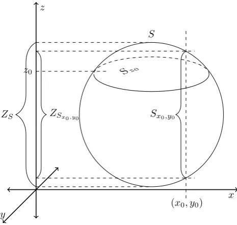
We will often refer to cylinders of S, i.e. preimages of the canonical pro-jections from S to its components X, Y, Z. If ˆZ ⊆Z, thenSZˆ ={(x, y, z) ∈

S : z ∈ Zˆ} is the cylinder above ˆZ and the corresponding notations for X

and Y. For singletons, we denote the cylinder above x0 ∈ X, y0 ∈ Y by

the following we will often call Sz the z-layer for any z ∈ Z. For the images

of the canonical projections, we denote XSˆ ={x∈X : (x, y, z)∈Sˆ}. We can

combine these notations,ZSx0,y0 ={z∈Z: (x0, y0, z)∈S}, etc..

S

S

z0

(x0, y0)

Sx0,y0

ZSx0,y0

x z

y ZS

Figure 1: Example of cylinder set notation

As an example (see Figure 1) consider a sphereSas a subset of the product spaceR3. Sz0is a disc where all points have the sameZcoordinate,z0, and may

also be called thez0-layer. Similarly,Sx0,y0 is an open segment of a vertical line.

ZSx0,y0 is the projection ofSx0,y0 to theZ dimension. If ¯Z ={z∈Z :z≥z0},

thenSZ¯ is the spherical cap abovez0.

% is a relation on S, i.e., a subset of S×S. We say that s is weakly preferred to s′ ifs%s′. We assume throughout the paper that%is complete and transitive and then call it a preference relation.2 _{Let≻be the strict part of}

%and∼the symmetric part. We say that two subsetsS′, S′′⊆S have strictly overlapping indifference curves if there exist points s, s′ _∈S′ _{and s}′′_{, s}′′′ _∈S′′

such that s≻s′_{, s}′′ _≻s′′′ _{and s%s}′′ _≻s′_{. A representation is a real valued}

functionu:S→Rsuch that u(s)≥u(s′_)⇔s%s′ _{for alls, s}′_{∈S and we say}

that urepresents %.

All topological concepts used in this paper (product and order topologies, connectedness, separability,. . . ) are standard definitions as can be found in Munkres (2014). To keep track of the different topologies and the continuity

2_{The results can possibly be generalized by dropping the completeness assumption. Vind}

properties of various functions, we introduce the following notation.

Definition 1. Topology notation:

i)tQi∈I∗Xi _{denotes the collection of all open sets induced by the product}

topol-ogy on the spaceQ i∈I∗Xi

ii) For a subset S⊆Qn i=0Xi,t

Q

i∈I∗Xi

S denotes the projections of all open sets

induced by the subspace topology oftQni=0Xi _toQ i∈I∗Xi

iii) For a subset S ⊆ Qn

i=0Xi and a relation % on Q n

i=0Xi, τS denotes the

collection of all open sets induced by the order topology generated by%onS.

Since we assume thatSis only a subset of a product space we require further conditions to ensure that this subset is well behaved. The following assumptions are adaptions from the requirements of Wakker and Chateauneuf (1993) to our setting.

Definition 2. The subsetS is well behaved givenZ if for allz∗ _∈Z

i)S is connected and open in tQni=1Xi

ii,a) for all i6∈IZ andx∗i ∈Xi {(s)∈S:xi=x∗i ∧z=z∗}is connected

ii,b)Sz∗ is connected

iii) all equivalence classes inint(Sz∗) are connected.

If the sphere in Figure 1 does not contain its boundary points, it fulfills the well behavedness assumptions subject to %fulfilling iii).

Our topological assumptions on each Xi guarantee that X, Y, Z are

con-nected, separable spaces. If X is a set of breakfast options this excludes finite sets such as X = {boiled egg,sandwich} but allows for sets which specify the weight or calorie value of the breakfast. For example, each x∈ X may be a statement of the kind “100 g of egg, 200 g of sandwich, 400 kcal total” making

X a subset of a three-dimensional vector space. However,X may also consist of lotteries over breakfast options. In this case,X is a function space and connect-edness and separability can be guaranteed by allowing the consumer to choose any mixture of available lotteries. Later, in Remark 2 and Lemma 8 we will argue that for the Z dimension finite sets such asZ ={vegetarian,beef,fish}

are also permissible.

The space S is an open subset of X ×Y ×Z. This means that choosing a certain breakfast may preclude the consumer to choose a certain dinner (for example due to financial or dietary constraints). The openness of S in the product topology is automatically implied in case S = X ×Y ×Z. Thus, a product of closed subsets ofRsuch as [0,400]×[0,900]×[0,1000] is permissible. Spaces excluded by this condition are for example spaces such as (x, y, z)∈R3_≥0

with the constraint x+y+z ≤ 100. The reason for this is the “Eiffel-tower problem” according to which on certain points of the boundary of S we may have infinite utility values. Wakker and Chateauneuf (1993) carefully discuss this problem and state conditions under which additive utility representations can be obtained also on closed subsets of product spaces. Our remaining well-behavedness assumptions imply the well well-behavedness assumptions of Wakker and Chateauneuf (1993) on every z-layer. In essence, “holes” in the space and cases where indifference curves are disconnected present problems for additive representability, and thus conditionally additive representability.3

Definition 3. Continuity:

%is continuous if the setsS(s) ={s′∈S:s′≻s}andS(s) ={s′ ∈S:s≻s′}

belong tot

Qn i=0Xi

S for alls∈S.

The continuity assumption is standard. It requires that for every alternative the sets of strictly better and strictly worse options are open in the subspace topology of the product topology.

Definition 4. Essentiality:

X is essential if for all x∈X there exist (y, z)∈ Y ×Z and (y′, z′)∈Y ×Z

such that (x, y, z)≻(x, y′, z′).

X is essential given Z if for all x ∈ X and all z ∈ Z there exist y ∈ Y and

y′∈Y such that (x, y, z)≻(x, y′, z).

%is essential ifX, Y, Z are essential.

%is essential givenZ ifX andY are essential givenZ.

Essentiality givenZ requires the choice of X and Y “to matter” at every point. Having an amazing dinner does not mean that breakfast is irrelevant. However, essentiality givenZ allows lunchZ to have no impact on preferences. Before we discuss the axioms driving our main result, it makes sense to revisit the standard axioms used in additive representation theorems.

Definition 5. Independence:

X is independent (ofY) if for allx, x′∈X andy, y′∈Y such that the following points are inS, we have:

(x, y)%(x′, y)

⇔ (x, y′)%(x′, y′). (4)

%is independent with respect toX andY ifX andY are independent.

Definition 6. Reidemeister Condition:

%fulfills the Reidemeister condition with respect toXandY if for allx, x′,x,¯ x¯′ ∈

X and ally, y′,y,¯ y¯′∈Y such that the following points are inS, we have:

(x, y)∼(¯x′,y¯′)

∧ (x′, y)∼(¯x,y¯′)

∧ (x, y′)∼(¯x′,y¯)

⇒ (x′, y′)∼(¯x,y¯). (5)

Together with continuity and essentiality, independence with respect toX

and Y, and the Reidemeister condition with respect to X and Y guarantee additive representability ofXandY (Wakker (1989), Wakker and Chateauneuf (1993)). We now present weakenings of the above two axioms which allow for conditionally additive representations.

Definition 7. Conditional independence:

X is independent (ofY) givenZ if for allx, x′ _{∈X,y, y}′_{∈Y, andz∈Z such}

that the following points are inS, we have:

(x, y, z)%(x′, y, z)

⇔ (x, y′, z)%(x′, y′, z). (6)

Independence given Z states that if a change in breakfast from xto x′ is beneficial, this change in X is beneficial independently of any change in the dinnery. Similarly, a change in dinner may not influence the preferences over breakfast. However, a change in breakfast or dinner may change the preferences over lunch options Z. For example, switching from no breakfast to a large breakfast may make large lunch options worse.

IfX is independent of (Y, Z), then X is independent ofY given Z. There-fore, our conditional independence axiom can be seen as a weakening of the independence axiom.

Definition 8. Coseparability:

%fulfills coseparability with respect toX andY givenZ if for allz,z¯∈Z and allx, x′_{,x,¯ x¯}′_{∈X and ally, y}′_{,y,¯ y¯}′_{∈Y such that the following points are inS,}

we have:

(x, y, z)∼(¯x′,y¯′,¯z)

∧ (x′, y, z)∼(¯x,y¯′,¯z)

∧ (x, y′, z)∼(¯x′,y,¯ ¯z)

⇒ (x′, y′, z)∼(¯x,y,¯ ¯z). (7)

Coseparability givenZ strengthens the notion of conditional independence. We can interpret coseparability as an independence in improvements and wors-enings. Suppose a change from (x, y, z) to (x′, y, z) yields an improvement which is as good as an improvement from (¯x,y,¯ z¯) to (¯x′,y,¯ z¯). Since we only changedx

tox′ and ¯xto ¯x′, these changes can be seen as improvements in the breakfast of the consumer. The indifferences imply that both improvements are equally ben-eficial. Similarly, the changes from (x, y, z) to (x′, y, z) and (¯x,y,¯ z¯) to (¯x,y¯′,z¯) can be seen as equally beneficial dinner improvements. Coseparability givenZ

holds if combining the breakfast and the dinner improvement for some lunch yields the same improvement as combining equally beneficial breakfast and din-ner improvements for another lunch. This is plausible in the case where im-provements in breakfast and dinner are comparable. If we instead assume X

and Y are the consumption of two different persons (and maybe Z their con-sumption of a public good), this ascon-sumption would imply cardinal comparability of preferences. In welfare analysis, many economists would feel comfortable as-suming conditional independence of the consumption of two persons but may not feel comfortable assuming cardinal comparability of their preferences. As a necessary condition for conditionally additive representability, it is important to consider whether one is indeed willing to commit to the coseparability condition before using a conditionally additive utility representation.

If%fulfills the Reidemeister condition with respect toX and (Y ×Z) then it fulfills coseparability ofX given Z, but not vice versa. Thus, coseparability is a weakening of the Reidemeister condition. However, assuming that%fulfills the Reidemeister condition with respect to X andY on every subspaceSz for

all z ∈ Z is weaker than coseparability given Z. This is why assuming an additive representation on each Sz only yields a global representation of the

To have a clean notation, we summarize conditional independence and cosep-arability in the following way.

Definition 9. To simplify notation, in the following we will writeX ⊥Y |Z if

• %is independent with respect toX andY givenZ and

• %fulfills coseparability with respect toX and Y given Z.

We say that % fulfills restricted solvability given Z if for all x, x′ _{∈ X,}

y, y′_{∈Y,z∈Z, ands∈S: If (x, y, z)%s%(x}′_{, y, z) then there existsx}′′_such

that (x′′_{, y, z)∼ s. If (x, y, z) % s %(x, y}′_{, z) then there exists y}′′ _{such that}

(x, y′′_{, z)∼s.}

3

Representation theorem for 3 dimensions

In this section, we will state our representation theorems for three dimensions and prove a lemma from which the main intuition of our result follows. The three dimensional case is the key building block for higher dimensional cases.

Theorem 1. Let%be a continuous preference relation on a well behaved space

S⊆X×Y ×Z. Let%fulfill essentiality givenZ. a) Then the following statements are equivalent:

(i) %fulfillsX ⊥Y |Z.

(ii) There exists a representation

v: (S, τS)→R,

f : (XS×ZS, tSXS×ZS)→R,

g: (YS×ZS, t_SXS×ZS)→R, and

v(x, y, z) =f(x, z) +g(y, z). (8)

b) v is continuous and unique up to positive affine transformations. f and g

are continuous ifZ is normal or ifZSx0,y0 =ZS. In the latter case,v(x, y, z) =

f(x, z) +g(y, z) +h(z) wheref(x0, z) = 0,g(y0, z) = 0 andf, g are unique up

to linear transformations andhis unique up to affine transformations.

Remark 1. If S = X ×Y ×Z, we do not need S to be well behaved. All assumptions summarized by S being well behaved are either trivially fulfilled by product spaces or not needed. In particular if each Sz is a product space

we can drop Definition 2 iii,b) which states that all indifference classes of a well behaved space need to be connected on each subset Sz.

Remark 2. According to our assumptions,Z is connected and separable. In-stead, we could also assume Z to be countable as long as for any two z0, zK

there exists a finite sequence (zk)Kk=1 of elements of Z such that for all k the

It is important to note that continuity off andgrequires further conditions. For most practical applications, the assumption of normality ofZ is not restric-tive. The main exception are function spaces from non-compact metric spaces to uncountable spaces. In additive representations, this problem never arises since we can replace the topology of each dimension with the order topology.

Due to its length, we delegate the proof of the representation theorem to the appendix with the exception of a Lemma which provides the main intuition behind the result and the proof of which links well with proofs of additive representations, in particular the proof of Theorem III.4.1. in Wakker (1989).

Lemma 1. Let %be a continuous preference relation onS=X×Y ×Z where

X, Y, Z are connected and separable topological spaces. Let%be essential given

Z and fulfillX ⊥Y |Z. Then: For any pair z′_{, z}′′ _{∈Z for which S}

z′ and S_z′′ have strictly overlapping

indif-ference curves there exists a utility representation on S{z′_,z′′_} such that: u(x, y, z) =f(x, z) +g(y, z) +h(z). (9)

We included Lemma 1 and its proof into the main text for two reasons. First, it gives an insight into the utility construction process and how this process differs from the procedure for additive representations. Second, Lemma 1 is of independent interest: it proves Remark 2 since given the result for twoz-layers, the extension to countably many layers is trivial.

Proof. We start out by constructing a utility function onSz′ =X×Y × {z′}.

We use the same utility construction process as in Wakker (1989). Using a standard argument, we can ensure%satisfies restricted solvability givenZ (see Lemma 2 in the appendix). Essentiality given Z guarantees that there exist

x0,x1∈X andy0 y1∈Y such that

(x0, y0, z′)≺(x1, y0, z′)

(x0, y0, z′)≺(x0, y1, z′)

(x1, y0, z′)∼(x0, y1, z′). (10)

By independence givenZ we have (x1, y1, z′)≻(x1, y0, z′)≻(x0, y0, z′) and we

assign utility values

u(x1, y1, z′) = 2, u(x1, y0, z′) = 1, u(x0, y0, z′) = 0. (11)

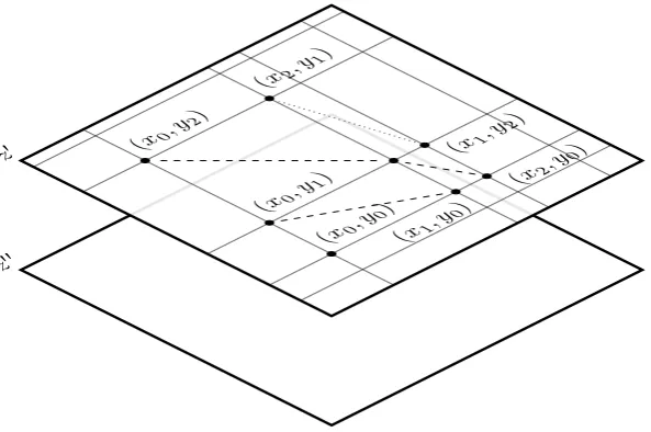
Next, since coseparability with respect to X and Y givenZ implies the Reide-meister condition with respect to X and Y on each z-layer X×Y × {z}, we can construct an order grid on the z′_{-layer such that for any rational numbers}

n, n′_{, m, m}′ _{we have}

(xn, ym, z′)∼(xn′, y_m′, z′)

⇔ u(xn, ym, z′) =n+m=n′+m′ =u(xn′, y_m′, z′). (12)

We provide an intuition for this construction process in Figure 2. For details of how to construct this grid, see Wakker (1989).

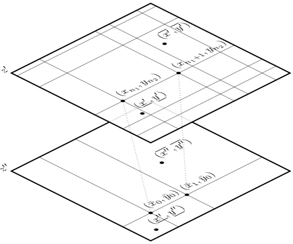
We next extend this representation to the z′′_{-layer (Figure 3). Since the}

indifference curves ofSz′ andS_z′′ strictly overlap, we can find points

(x′_{, y}′_{, z}′₎

%(x′′_{, y}′′_{, z}′′_)≻(

z

(

x

, y

)

(

x

, y

)

(

x

, y

1

)

(

x

, y

)

(

x

, y

0

)

(

x

, y

)

(

x

, y

1

)

z

Figure 2: Construction of the utility grid on thez′-layer.

By restricted solvability given Z, the points (x0, y1, z′), (x1, y0, z′) are chosen to be

in-different to each other. Similarly, the points (x0, y2, z′), (x2, y0, z′) are chosen to be

indifferent to (x1, y1, z′) (dashed indifferences). Coseparability given Z then guarantees

(x2, y1, z′) ∼ (x1, y2, z′) (dotted indifference). These indifferences allow us to guarantee

(xn, ym, z′)∼ (xn′, ym′, z′) iff n+m= n′+m′. In a next step, this grid is made dense

inSz′.

Since our grid is dense in thez′-layer, we can find a grid point (xn1, yn2, z

′_{) on}

thez′-layer such that (x′, y′, z′)≺(xn1, yn2, z

′_)≺(x′_{, y}′_{, z}′_{). Therefore, by}

re-stricted solvability givenZ, we can find a point (¯x,y, z¯ ′′)∼(xn1, yn2, z

′_{). Next,}

we construct the grid on both z-layers in the following way. We use the point (¯x0,y¯0, z′′) on the z′′-layer satisfying (¯x0,y¯0, z′′)∼ (xn1, yn2, z

′_{) as the center}

on the z′′-layer and construct the grid with an initial point ¯x1,y¯0 satisfying

(¯x1,y¯0, z′′)∼(xn1+1, yn2, z

′_{). These points exist by restricted solvability given}

Zand by the fact that we can choose our initial points (x0, y0, z′) and (x1, y0, z′)

to be arbitrarily close to each other.

We now show that the grid points are indeed consistent on both layers (Fig-ure 4). That is, we want to show that

(xn+1, ym, z′)∼(xn, ym+1, z′)

(¯xn+1,y¯m, z′′)∼(¯xn,y¯m+1, z′′)

(xn, ym, z′)∼(¯xn1+n,y¯n2+m, z

′′_{) (14)}

for alln, m.

Similar to the argument of Wakker (1989), we use induction on our subcripts. For n+m = 0, the result directly follows from (¯x,y, z¯ ′′) ∼(xn1, yn2, z

′_{). For}

z

(

x

, y

′′

)

(

x

, y

′′

)

(¯

x

,

y

¯

) (

x

¯

,

y

¯

)

(

x

, y

n2

)

(

x

, y

)

(

x

, y

′

)

(

x

, y

)

z

Figure 3: Extension of the utility grid from thez′ layer to thez′′layer.

The existence of points (xn1, yn2) and (xn1+1, yn2) such that both are worse than (x

′′_{, y}′′₎

and better than (x′′_{, y}′′_{) follows from the gridpoints being dense inS}

z′. The existence of the

points (¯x0,y¯0) and (¯x1,y¯0) follows from restricted solvability givenZ. indifferencexn1, yn1∼

(¯x0,y¯0)

we simply notice that coseparability givenZ implies

(xn1+n−2, yn2, z

′_)∼(¯

xn−2,y¯0, z′′)

(xn1+n−1, yn2, z

′_)∼(¯x

n−1,y¯0, z′′)

(xn1+n−2, yn2+1, z

′_)∼(¯x

n−2,y¯1, z′′)

and therefore (xn1+n−1, yn2+1, z

′_)∼(¯x

n−1,y¯1, z′′). (15)

We can extend the integer-valued grid on thez′′_{-layer to a rational-valued}

grid by the same method as in Wakker (1989). Via transitivity and the fact that for any xn, n ∈ Q we can find ym such that there exist xn′, n′ ∈ Z and ym′, m′ ∈Z such thatn+m=n′+m′ and thus (x_n, y_m, z′′)∼(x_n′, y_m′, z′′),

the extended grid on the rationals is also consistent. Next, we define the functions

f(xn, z′) :=n

f(¯xn, z′′) :=n

g(ym, z′) :=m

g(¯ym, z′′) :=m

h(z′′) :=n1+n2

z

(¯

x

,

y

¯

)

(¯

x

,

y

¯

)

(¯

x

,

y

¯

0

)

(¯

x

,

y

¯

)

(

x

, y

n2

)

(

x

, y

n2+1

)

(

x

, y

)

(

x

, y

)

z

Figure 4: Consistency of the utility grid between thez′-layer and thez′′-layer.

The dashed indifferences follow from the construction process of the grid. The dashed indif-ference follows from coseparability givenZ.

Since our grid is dense in thez′ andz′′-layers, due to continuity we can extend the utility functions on the entirez′andz′′-layers by taking the limit to obtain a continuous additive utility representationu(x, y, z) =f(x, z) +g(y, z) +h(z) on both layers.

In summary, the construction of the utility representation on a single layer follows the construction by Wakker (1989). In this step, our coseparability condition fulfills the same role as the Reidemeister condition in Wakker (1989): if a preference relation over a product spaceX×Y is continuous, essential, and independent, the Reidemeister condition is necessary and sufficient to ensure that an additive representation exists.

When extending the representation to the second layer, coseparability given

Zfulfills an additional role: it makes the additive representations on both layers consistent with each other. Assuming only the Reidemeister condition on each

Sz without our generalization, we could obtain an additive representation on

each Sz. But notice that for example the preference relation induced by the

utility function (f(x) +g(y))h(z)_{has an additive representation on eachz-layer,}

4

Representation theorems for finitely many

di-mensions

In the following, we will extend our representation result to product spaces of higher dimensions. Notice that as soon as there are more than three dimen-sions, different extensions are possible. In terms of utility functions, we may for example be interested in the conditions which yield a representation of the kind

f(x2, x1) +g(x3, x1) +h(x4, x1) or insteadf(x1, x2) +g(x2, x3) +h(x3, x4). In

the following, we will consider some cases we found interesting. We hope that our treatment of these cases is instructive for the cases we omit.

4.1

Reference dependent preferences

We start out with the simplest generalization to finite dimensional spaces, the case where we have a conditionally additive representation onn−1 dimensions given the first dimension. We call these preferences reference dependent as we can interpret the first dimension as a reference point by which the remaining dimensions are evaluated.

Theorem 2. Let%be a continuous preference relation on a well behaved space

S ⊆Z×Qn

i=1Xi, 2≤i <∞ where allXi and Z are connected and separable

topological spaces. Let % be essential given Z. Then the following statements are equivalent:

(i) %fulfills for alli:

• Xi⊥Q_j6=iXj |Z and

• Xi×Xi+1⊥Qk6=i,i+1Xk |Z.

(ii) %can be represented by a continuous functionv(s) =Pn

i=2fi(xi, z)unique

up to affine transformations.

Remark 3. Continuity of the additive components fi can be guaranteed in a

similar manner as in Theorem 1 by assuming normality of Z orZSx0,y0 =ZS.

In order to extend our results to more than three dimensions we need to impose additional independence conditions Xi×Xj ⊥. . . | Z. This is

unsur-prising given the work of Gorman (1968). Without the additional conditional independence assumptions, additive representations on each z-layer may not exist.

Sugden (2003) axiomatizes reference dependent preferences in a Savage (1972) framework. Due to the differences in the framework, it is hard to compare the two models in their generality. One difference is that our representation is ad-ditive given the reference point, while Sugden (2003) axiomatizes a (reference dependent) subjective expected utility representation. Sugden (2003) allows for an uncountable event space as opposed to the finite number of dimensions in our space. The functional form axiomatized by Sugden (2003) is therefore neither a special case nor a generalization of Theorem 2.

We now provide an example application where we derive a generalization of previous axiomatizations of Fehr and Schmidt (1999) using Theorem 2. In a product spaceQ

and Schmidt (1999) inequity aversion preferences of individualiare represented by a utility function of the form:

ui(s) =xi− X

j6=i

αimax(0, xj−xi)−βimax(0, xi−xj). (17)

Rohde (2010) axiomatized the functional form of Fehr and Schmidt (1999) using the strong linearity assumptions fulfilled by the model. The linearity assumptions prescribe (i) indifference about redistribution of income among individuals with better income, and (ii) redistribution among indiviudals with worse incomes. Neilson (2006) provides a more general representation theorem by dropping linearity of the model but maintaining linearity in the comparisons between individuali’s and any otherj’s income. One avenue for generalizations mentioned in Rohde (2010) are rank-dependent utility models. Here, we try the conditionally additive utility approach.

It is straightforward to obtain the representationu(x1, . . . , xn) = ui(xi) + P

j∈I\{i}uj(xj, xi) via Theorem 2. Having obtained such a representation, the

remaining axioms for a theory of inequity aversion easily fall into place.

Definition 10. Anonymity: Ifs, s′_∈Q

i∈IXi,xi=x′i ands′ is a perturbation ofs, thens∼s′.

This axiom requires that the individual cares about others’ incomes in an identical manner. The neighbor’s income, for example, has exactly the same effect on the individual’s income as the income of any other person.

Definition 11. Envy:

If for allj, k6=iwe havexj> xj≥xi, then

(x1, . . . , xj−1, xj, xj+1, . . . , xn)≻(x1, . . . , xj−1, xj, xj+1, . . . , xn).

The envy axiom implies that the individual cares negatively about anybody’s income exceeding their own.

Definition 12. Compassion:

If for allj, k6=iwe havexi≥xj > xj then

(x1, . . . , xj−1, xj, xj+1, . . . , xn)≻(x1, . . . , xj−1, xj, xj+1, . . . , xn).

The compassion axiom means that an individual cares positively about anybody’s income below their own income. Envy and compassion are slight strengthenings of the inequity aversion axiom in Rohde (2010).

Corollary 1. Let S =Qn

i=1Xi, and %be a continuous preference relation on

S. Let%be essential givenXi. Then the following statements are equivalent:

(i) %fulfills symmetry, envy, compassion, and for allj, k:

• Xj⊥Q_k6=i,jXk|Xi and

• Xj×Xj+1⊥k6=i,j,j+1Xk|Xi.

(ii) %can be represented by:

u(x) =v(xi) + X

j6=i

u(xj, xi) (18)

whereuis continuous and strictly increasing (strictly decreasing) inxj if

The usefulness of Theorem 2 is the simplicity with which this result can be proven. We provide the proof directly:

Proof. From Theorem 2, we have that%can be represented by:

u(x1, . . . , xn) =v(xi) + X

j∈I\{i}

uj(xj, xi).

Using a perturbation of the incomes of three individualsj, k, l, we have

uj(xj, xi) +uk(xk, xi) =uj(xk, xi) +uk(xj, xi)

uj(xj, xi) +ul(xl, xi) =uj(xl, xi) +ul(xj, xi)

uk(xk, xi) +ul(xl, xi) =uk(xl, xi) +ul(xk, xi).

Ifxj =xl=x∗it is straightforward to deriveuj(x∗, xi)−uk(x∗, xi) is constant.

Since our choice ofx∗_{, x}

i, k, l was arbitrary and eachuk is unique up to affine

transformations, we have for allk, l: uk =ul=u. Thus,

u(x1, . . . , xn) =v(xi) + X

j∈I\{i}

u(xj, xi).

The fact thatumust be increasing/decreasing in its second argument forxj<

(>)xi follows directly from the remaining axioms.

Theorem 2 directly provides us with a functional form on which we can impose axioms descriptive of the behavior we are interested in. The gener-alization of the functional form of (17) would be of little interest if it could not capture some plausible deviations from the behavior implied by (17). One such deviation is a preference against inequity among the individuals poorer than oneself. Suppose the individuals are ordered by their income such that

x1 ≤x2 ≤. . . ≤xn. The linear structure of (17) forces individual i to have

preferences (0, . . . ,0, xi−1, xi, . . . , xn)∼( xi−1

i−1, . . . , xi−1

i−1, xi, . . . , xn). Instead, we

may want to impose that the individual also cares negatively about inequity of incomes below herself. We can do this by assuming:

x≻(x1−α, x2+α, x3, . . . , xi, . . . , xn) (19)

for all x andα∈ R>0 such that x2+α≤xi andx2 ≤x1. It is then easy to

show that u(xj, xi) is strictly concave inxj forxj≤xi.

4.2

Dynamic dependence preferences

The previous subsection covers the case where all additive component functions

fi share one argument z. Another interesting representation arises if for all

i we assume that the first i−1 dimensions are independent of the last n−i

dimensions given the i-th dimension.

Theorem 3. Let%be a continuous preference relation on a well behaved space

S ⊆ Qn

i=1Xi, 3 ≤ i < ∞ where all Xi are connected and separable

topolog-ical spaces. For all i, let % fulfill essentiality given Xi. Then the following

statements are equivalent:

(i) %fulfills for alli= 2, . . . , n−1: Qi−1

j=1Xj⊥Q n

k=i+1Xk|Xi.

(ii) %can be represented byv(s) =Pn

Remark 4. Continuity of each fi can be guaranteed by eachXi being normal

or S being a product space.

A natural application for this representation theorem are preferences over time which exibit dependence across time periods. Preferences over consump-tion streams need not be additively separable if individuals experience satiaconsump-tion and addiction, or form consumption habits (a growth model with time inter-dependence is given in Ryder and Heal (1973), for an axiomatization of habit preferences, see Rozen (2010)). In this case, preferences over consumption peri-ods sufficiently distant in time may be additively separable when holding fixed the consumption in between. The above representation theorem captures the case where the marginal utility of consumption depends on the previous period’s consumption. The overlapping number of dimensions can of course be increased by a corresponding change in the independence conditions.

More generally, time preferences provide a rich field of applications for our main theorem in deriving axiomatizations in the spirit of Theorem 3. For exam-ple, we may consider preferences as in Kydland and Prescott (1982) (for finite time periods):

n X

i=0

βiu(xi, i X

j=1

αiyi) (20)

wherexiis consumption at timei,yiis leisure at timei, andαi is a preference

parameter. Using the exact same method of proof as in Theorem 3 we invite the reader to derive:

Corollary 2. Let %be a continuous preference relation onS=Qn

i=1Xi×Yi,

3≤i <∞where for alli Xi=RandYi=R. For alli, let%fulfill essentiality

givenQi

l=1Yl. Then the following statements are equivalent:

(i) %fulfills for alli= 1, . . . , n−1: Xi⊥Q n

j6=iXj×Qn_k=i+1Yk |Qi_l=1Yl.

(ii) % can be represented by v(s) = Pn

i=1fi(xi, y1, . . . , yi) where each fi is

continuous.

The common element in Theorem 3 and Corollary 2 is that both representa-tions originate from combining additive representarepresenta-tions in a sequential manner. In Corollary 2 each statement . . . ⊥ . . . | . . . tells us for some dimension i

which of the i−1 dimensions before andn−idimensions after are condition-ally independent. Theorem 1 gives us conditioncondition-ally additive representations for each of these statements. The proof of Theorem 3 shows how to combine such representations into a dynamically dependent representation.

4.3

Rank dependent preferences

Lastly, we can obtain a generalization of dependent expected utility. Rank-dependent expected utility (Quiggin (1982)) has a representation:

n X

i=1

(v(yi)−v(yi−1))u(xi) (21)

where for alli= 1, . . . , neachxiis a payoff andyiis the probability of receiving

Theorem 4. Let (X,⋗),(Y,⋗) be ordered, connected, separable spaces en-dowed with the order topology induced by ⋗. Assume a well behaved space

S⊆Qn

i=1Xi×Yi such that for all i Xi=X,Yi=Y and:

(x1, y1, . . . , xn, yn)∈S⇔ ∀i∈ {1, . . . , n−1}:xi+1⋗xi, yi+1⋗yi. (22)

Let % be a continuous preference relation on S fulfilling for all i essentiality givenXi. Then the following statements are equivalent:

(i) For all i= 2, . . . , n−1 the relation%fulfills

Xi× i−1 Y

j=1

Xj×Yj⊥ n Y

k=i+1

Xk×Yk|Yi, and

i−1 Y

j=1

Xj×Yj ⊥Yi× n Y

k=i+1

Xk×Yk|Xi. (23)

(ii) %can be represented by:

v(s) =

n X

i=1

fi(xi, yi) +gi(xi, yi−1) (24)

where eachfi andgi is continuous.

For the connection to Rank-dependent Expected Utility, suppose X = R,

Y = [0,1]⊂R, and the subsetS is chosen such that for alliwe havexi< xi+1,

yi< yi+1. xican be interpreted as theith lowest prize andyi as the probability

of receiving a prize lower or equal to xi. Then setting fi(xi, yi) = u(xi)w(yi)

and gi(xi, yi−1) = −u(xi)w(yi−1) gives the familiar rank-dependent expected

utility form. In fact, the representation is more general than Rank-linear utility first axiomatized in Segal (1989) (see also Puppe (1990); Wakker (1993); Segal (1993)). Rank-linear utility can be obtained by removing the subscript fromfi

andgi.

Theorem 4 only generalizes rank-dependent utility models for decisions un-der risk where the probabilities are known. Thus, the above result holds only for decisions under risk but not uncertainty. However, many results on rank-dependent representations for decisions under uncertainty with unknown proba-bilities are derived using additive representation theorems.4 _{It would be}

interest-ing to apply conditionally additive representation theorems to rank dependent models of decisions under uncertainty.

5

Finite dimensional simplices

We can use Theorem 1 to provide an interesting new result on additive rep-resentations. So far, additive representations have only been axiomatized for sets with nonempty interiors in the product topology. However, an important class of spaces in economics which do not fulfill this requirement are simplices

4

of the form {(x1, . . . , xn) ∈ Rn : P n

i=1xiθi = 1}. We encounter simplices

for example in lottery spaces, as income shares in fair division problems, or as normalized price vectors. The literature lacks a result for such spaces be-cause in this context the classical independence axiom is not well defined when looking at the independence of a single dimension. Take a statement such as (x, y)%(x′, y)⇒(x, y′)%(x′, y′) wherexis the first dimension of the simplex andy the remaining dimensions. Then by the properties of the simplex,x=x′

and the axiom is not meaningful. However, even if we consider xto contain more than one dimension, we run into difficulties. To show why, let us focus on a 4 dimensional simplex and let x= (x1, x2) contain the first two dimensions

and y = (x3, x4) contain the other two dimensions. Now a statement such as

(x, y)%(x′_{, y) ⇒(x, y}′_)%(x′_{, y}′_{) only imposes restrictions on preferences on}

the subset of alternatives wherex1+x2=x′1+x′2. Yet, this is exactly the case

where conditionally additive representation theorems become useful.

Indeed, Theorem 1 helps us find conditionally additive representations of the form f(x1, x1+x2) +g(x3, x1+x2). To see this, consider the following

preferences%∗ on a subset of a product set (0,1)3_:

(x1, x2, x3, x4) = (x, y)%(x′, y′) = (x′1, x′2, x′3, x′4)

⇔ (x1, x3, x1+x2)%∗(x′1, x′3, x′1+x′2). (25)

It is straightforward to verify that independence ofX andY in the relation %

implies conditional independence ofX1 andX3 givenX1+X2in %∗:

(x1, x3, x1+x2)%∗(x′1, x3, x′1+x′2)

⇔ (x, y)%(x′, y)

⇔ (x, y′)%(x′, y′)

⇔ (x1, x′3, x1+x2)%∗(x′1, x′3, x′1+x′2) (26)

ifx1+x2=x1′ +x′2. Similarly, the Reidemeister condition of X and Y in the

relation%implies coseparability givenX1+X2of%∗. Together with essentiality

we obtain the representationf(x1, x1+x2) +g(x3, x1+x2) of%∗ and thus%.

In the same fashion we can obtain a representation ¯f(x1, x1+x3)+ ¯g(x2, x1+

x3). The existence of the two representations of the same relation gives us the

functional equation

for some monotone transformation T. However, this does not yet guarantee additive representability. To make the representation additive among all di-mensions, we need to introduce an additional axiom.

Definition 13. Comeasurability:

(Xi, Xn) and (Xj, Xn) are comeasurable if for allxi,xj,xk,xn,x′i,xj′,x′k,x′n,

x′′

i, x′′j,x′′k,x′′n for which the following elements ofS are defined:

((xl)l6=i,j,k,n, x′i, xj, xk, x′n)

∼((xl)l6=i,j,k,n, xi, x′j, x ′ k, xn)

∼((xl)l6=i,j,k,n, xi, x′′j, xk, x′′n)

∼((xl)l6=i,j,k,n, xi′′, xj, x′′k, xn)

⇒

((xl)l6=i,j,k,n, x′i, x′j, x′k, x′n)

∼((xl)l6=i,j,k,n, x′′i, x′′j, x′′k, x′′n). (28)

Comeasurability is very similar to the Reidemeister condition. In fact, if we set

x= (xi, xn) y= (xj, xk)

¯

x= (xi, xk) y¯= (xj, xn)

x′= (x′i, x′n) y′ = (x′j, x′k)

¯

x′= (x′′i, x ′′

k) y¯= (x ′′ j, x

′′

n) (29)

in (5) then it becomes apparent that for a four-dimensional simplex, comeasur-ability is simply the Reidemeister condition with a change of dimensions when comparing the LHS to the RHS of (5). Comeasurability guarantees that in the four-dimensional case discussed above, T is affine. In Lemma 12 we solve the functional equation (27) for affine T using a result from Hossz´u (1971).

We obtain the following representation theorem.

Theorem 5. SupposeS = {x∈ Qn

i=1Xi : xn = 1−Pn−1_i=1 xi} and for all i,

Xi= (0,1). Let%be a continuous preference relation fulfilling for all i, j:

• (Xi, Xn)andQ_k6=i,nXk are independent,

• (Xi, Xn)andQk6=i,nXk are essential,

• (Xi, Xn)andQk6=i,nXk fulfill the Reidemeister condition,

• comeasurability of(Xi, Xn)and(Xj, Xn).

Then%can be represented by a continuous functionu: (S, τ

Qn

i=1Xi

S )→R:

u(x) =

n X

i=1

ui(xi). (30)

Remark 5. We can continuously extend the representation to the closure of the simplex except points where for some i, xi = 1, since it may be that

This result is very similar to additive representation theorems on product spaces. The only differences are that the independence, essentiality, and Reide-meister conditions have been imposed on pairs of dimensions instead of single dimensions and the additional use of comeasurability between these pairs of dimensions.

Theorem 5 provides an axiomatization for Utilitarianism in cake division problems. In a cake division problem, a fixed resource is divided among n

individuals. If we normalize the amount of the resource to 1, we havePn i=1xi=

1 as a constraint. Therefore, the space on which preferences are defined is an n-dimensional simplex.5 _{If the decision maker’s preference is consistent with}

the axioms in Theorem 5, the decision maker is consistent with Utilitarianism in the following sense. For each individual i, the decision maker can find a utility function ui, which is cardinally comparable to the utility function of

any other j. The decision maker ranks allocations according to the sum of the utility functions. This result can be generalized to cases where agents differ in their productivity with which they convert the resource into some consumption product:

Remark 6. Theorem 5 holds for any spaceS′ where we can find a homeomor-phism h : S′ →S such that h(s′) = h(x′1, . . . , x′n) = (h1(x1′), . . . hn(x′n)) and

eachhi is a homeomorphism.

This follows from the fact that our independence, essentiality, coseparability, and comeasurability assumptions do not refer in any way to the linear structure of a simplex. In our cake division problem we could assume that each individual

i transforms the resource by multiplying it with a productivity parameter θi.

Then Theorem 5 holds forS′_={x∈Qn

i=1Xi:θnxn = 1−Pn−1_i=1 θixi}.

Naturally, it is interesting to consider a reference-dependent version of the Theorem 5. For this, we need to extend the definition of comeasurability to a conditional version:

Definition 14. Conditional Comeasurability:

(Xi, Xn) and (Xj, Xn) are comeasurable givenZif for allxi,xj,xk,xn,x′i,x′j,

x′k,x′n,x′′i,x′′j,x′′k,x′′n for which the following elements ofS are defined:

((xl)l6=i,j,k,n, x′i, xj, xk, x′n, z)

∼((xl)l6=i,j,k,n, xi, x′j, x′k, xn, z)

∼((xl)l6=i,j,k,n, xi, x′′j, xk, x′′n, z)

∼((xl)l6=i,j,k,n, x′′i, xj, x′′k, xn, z)

⇒

((xl)l6=i,j,k,n, x′i, x ′ j, x

′ k, x

′ n, z)

∼((xl)l6=i,j,k,n, x′′i, x ′′ j, x

′′ k, x

′′

n, z). (31)

5

Corollary 3. Suppose S ={x∈Qn

i=1Xi : xn = 1−P n−1

i=1 xi} and for all i:

Xi= (0,1). Z is a connected, separable topological space. Let%be a continuous

preference relation on S×Z fulfilling for all i, j:

• essentiality givenZ,

• Xi×Xn⊥Q_k6=i,nXk |Z,

• conditional comeasurability of(Xi, Xn)and(Xj, Xn) givenZ.

Then%can be represented by:

u(x, z) =

n X

i=1

ui(xi, z). (32)

This shows that our previous results for conditionally additive representa-tions carry over to simplices under the additional assumption of comeasurability.

6

Mixture Spaces

In some cases, we are interested in even stronger independence conditions which generate not only additive, but linear utility functions. The classical example is expected utility axiomatized by von Neumann and Morgenstern (1944). Her-stein and Milnor (1953) generalize their results to mixture spaces, which we will study in the following.

LetZ be a connected, separable set and S an arbitrary set. Letξ:S →Z

be continuous. For eachz∈Z we assume a setSz={s∈S :ξ(s) =z}with an

operator⊕such that for alls, s′ ∈S andµ, λ∈[0,1]⊆Rwe have:

µs⊕(1−µ)s′ ∈Sz

1s⊕0s′ =s

µs⊕(1−µ)s′ = (1−µ)s′⊕µs

λ(µs⊕(1−µ)s′)⊕(1−λ)s′ = (λµ)s⊕(1−λµ)s′. (33)

We call (S, Z,⊕) a conditional mixture space. We call it a continuous conditional mixture space if for all s, s′ _{∈ S the map α7→ αs⊕(1−α)s}′ _{is a continuous}

map.

Naturally, conditional independence in this context means:

Definition 15. Conditional independence:

For mixture spaces,%is conditionally independent givenZ if for allz∈Z and alls, s′, s′′∈Szand allµ∈[0,1]:

s∼s′⇔ 1

2s⊕ 1 2s

′′_∼1

2s

′_⊕1

2s

′′_{. (34)}

As usual, we need the technical assumption of essentiality to avoid some pathological cases.

Definition 16. Essentiality:

For mixture spaces, %is essential givenZ if for allz∈Z there exists, s′∈Sz

The coseparability condition for product spaces can be translated to this context as:

Definition 17. Coseparability:

For mixture spaces,%fulfills coseparability givenZ if for all z,z¯in Z:

s∼y¯ 1

2s⊕ 1 2s

′ _∼1

2s¯⊕ 1 2¯s

′

1 2s⊕

1 2s

′′_∼1

2s¯⊕ 1 2¯s

′′

⇒ 1

2s

′_⊕1

2s

′′_∼1

2s¯

′_⊕1

2s¯

′′ ₍₃₅₎

wheres, s′, s′′∈Sz and ¯s,s¯′,s¯′′∈Sz¯.

Compared to the earlier definition, we have slightly simplified the exposition due to the commutativity of⊕.

Theorem 6. Suppose(S, Z,⊕)is a continuous conditional mixture space and%

is a continuous preference relation onS. Let %fulfill the following conditions:

• conditional independence givenZ,

• essentiality givenZ, and

• coseparability givenZ.

Then there exists a representation u:S →R and functions uz :Sz→R such

that

u(s) =uξ(s)(s) (36)

uz(µs⊕(1−µ)s′) =µuz(s) + (1−µ)uz(s′) (37)

for alls, s′∈Sz and allµ∈[0,1].

Remark 7. If S = Qn

i=1Xi×Z = Rn×Z, ξ(x1, . . . , xn, z) = z and ⊕ is

defined as vector summation for elements with identical z ∈ Z, then u(s) =

Pn

i=1xiui(z).

We apply Theorem 6 to decisions under risk and uncertainty. SupposeZis a set of acts with uncertain (and possibly unknown) consequences. x1, . . . , xn are

In the above axiomatization, we impose von Neumann Morgenstern prefer-ences over lotteries when holding the act z fixed. Coseparability ensures com-parability of the von Neumann Morgenstern preferences across different actsz,

z′. Under these more stringent assumptions on the preferences given Z, the coseparability condition is a powerful, yet highly plausible axiom for rational decision makers. If a decision maker maximizes the expectation of her experi-enced utility given a decision z, then there is no good reason to believe that this expectation of the experienced utility should not be comparable with that given a decisionz′_.

In particular, coseparability forbids separate “utility accounts” for z and

x1, . . . , xn: suppose the decision maker first determines the utility of the lottery

and in a second step transforms this utility depending on the actzusing a non-linear function. Then the utility function would instead beu(s) =v(P

ixiui, z).

We may call this a case of two “utility accounts” as the decision maker first forms an account for the utility of the lottery and then combines this utility with the utility from the actz. An example of an axiomatization which allows for such behavior is given in Karni (2006) where thev function may be nonlinear. In-stead, coseparability forces the decision maker to separately consider the utility from each outcome i given act z and take the expectation over these utilities

ui(z).

A special feature of this axiomatization apart is the lack of a specification of how acts relate to outcomes.6 _{This is intuitive for applications where there}

may be unforeseen consequences of acts or where due to bounded rationality it is impossible for a decision maker to relate acts, outcomes, and states of the world. If our axioms are accepted, a decision maker facing a situation where some outcomes are unknown should (when holding fixedz) behave in line with expected utility for simultaneous choices over lotteries and should be able to cardinally compare the expected utility functions across different acts z,z′_.

References

Abdellaoui, M. (2009). Rank-Dependent Utility. In Anand, P., Pattanaik, P. K., and Puppe, C., editors, The Handbook of Rational and Social Choice, pages 69–89. Oxford University Press, Oxford, UK.

Chew, S. H. and Sagi, J. S. (2008). Small worlds: Modeling attitudes toward sources of uncertainty. Journal of Economic Theory, 139(1):1–24.

Debreu, G. (1959). Topological Methods in Cardinal Utility Theory. In Arrow, K. J., Karlin, P., and Suppes, P., editors,Mathematial Methods in the Social Sciences, pages 16–26. Stanford University Press, Stanford.

Dr`eze, J. H. and Rustichini, A. (1999). Moral hazard and conditional prefer-ences. Journal of Mathematical Economics, 31(2):159–181.

Fehr, E. and Schmidt, K. M. (1999). A theory of fairness, competition, and cooperation. The quarterly journal of economics, 114(3):817–868.

6

Gorman, W. M. (1968). The Structure of Utility Functions. The Review of Economic Studies, 35(4):367–390.

Herstein, I. N. and Milnor, J. (1953). An Axiomatic Approach to Measurable Utility. Econometrica, 21(2):291–297.

Hossz´u, M. (1971). On the functional equation

F(x+y,z)+F(x,y)=F(x,y+z)+F(y,z). Periodica Mathematica Hungarica, 1:213–216.

Karni, E. (1998). The Hexagon Condition and Additive Representation for Two Dimensions: An Algebraic Approach. Journal of Mathematical Psychology, 42:393–399.

Karni, E. (2006). Subjective expected utility theory without states of the world.

Journal of Mathematical Economics, 42(3):325–342.

Kydland, F. E. and Prescott, E. C. (1982). Time to Build and Aggregate Fluctuations. Econometrica, 50(6):1345–1370.

Munkres, J. (2014). Topology. Pearson, Essex, UK.

Neilson, W. S. (2006). Axiomatic reference-dependence in behavior toward oth-ers and toward risk. Economic Theory, 28(3):681–692.

Puppe, C. (1990). The irrelevance axiom, relative utility and choice under risk.

Quiggin, J. (1982). A Theory of Anticipated Utility. Journal of Economic Behavior and Organization, 3:323–343.

Reidemeister, K. (1929). Topologische Fragen der Differentialgeometrie. V. Gewebe und Gruppen. Mathematische Zeitschrift, 29(1):427–435.

Rohde, K. I. M. (2010). A preference foundation for Fehr and Schmidt’s model of inequity aversion. Social Choice and Welfare, 34(4):537–547.

Rozen, K. (2010). Foundations of Intrinsic Habit Formation. Econometrica, 78(4):1341–1373.

Ryder, H. E. and Heal, G. M. (1973). Optimal Growth with Intertemporally Dependent Preferences. The Review of Economic Studies, 40(1):1–31. Savage, L. J. (1972). The Foundations of Statistics. Courier Corporation. Segal, U. (1989). Anticipated utility: A measure representation approach.

An-nals of Operations Research, 19(1):359–373.

Segal, U. (1992). Additively Separable Representation on Non-convex Sets.

Journal of Economic Theory, 56:89–99.

Segal, U. (1993). The measure representation: A correction. Journal of Risk and Uncertainty, 6(1):99–107.

Tversky, A. and Kahneman, D. (1992). Advances in prospect theory: Cumula-tive representation of uncertainty. Journal of Risk and uncertainty, 5(4):297– 323.

Vind, K. (1991). Independent preferences. Journal of Mathematical Economics, 20(1):119–135.

von Neumann, J. and Morgenstern, O. (1944). Theory of Games and Economic Behavior. Princeton University Press.

Wakai, K. (2007). Risk Non-Separability without Force of Habit.

Wakker, P. (1993). Counterexamples to Segal’s measure representation theorem.

Journal of Risk and Uncertainty, 6(1):91–98.

Wakker, P. and Chateauneuf, A. (1993). From local to global additive repre-sentation. Journal of Mathematical Economics, 22:523–545.

Wakker, P. and Tversky, A. (1993). An axiomatization of cumulative prospect theory. Journal of risk and uncertainty, 7(2):147–175.

Wakker, P. P. (1989). Additive Representations of Preferences: A New Founda-tion of Decision Analysis, volume 4. Springer Science & Business Media. Wang, T. (2003). Conditional preferences and updating. Journal of Economic

Appendix A

Proof of Theorem 1

Necessity of the conditions for the representation and the uniqueness properties are trivial. We therefore focus on proving sufficiency. In the steps up to Lemma 6 we show that for every interior indifference curve we can find a point such that there exists a basic open setO=Ox×Oy× {z} ⊆Szcontaining the point

and points strictly better and worse. This ensures that across differentz-layers we can make the conditionally additive representations consistent using 1. In the following steps to Lemma 9 we show sufficiency for the existence of the representationv. The remainder of the proof derives the continuity properties.

A standard result used throughout this paper is:

Lemma 2. Suppose%is a continuous preference relation onS fulfilling essen-tiality givenZ. Then%satisfies restricted solvability givenZ.

Proof. We can simply apply the proof of Wakker (1989) Lemma III.3.3. to each

Sz.

Definition 18. A points= (x, y, z) is called locallyX-nonsatiated if for every open setO∈tX×YSy,z ×Z containingsthere exists a points

′ _{= (x}′_{, y, z)∈O such}

that s′≻s.

s = (x, y, z) is called locally X, Y-nonsatiated if it is X-nonsatiated and Y -nonsatiated.

Lemma 3. Suppose S ⊆ X ×Y ×Z is well behaved given Z. Let % be a continuous preference relation on S with a continuous representation u. Then for everyi∗_∈u(S

x,z)such thati∗6= maxs∈Sx,zu(s)there exists a points∈Sx,z

such that u(s) =i∗ _{ands is locallyY-nonsatiated.}

Proof. We prove the result by contradiction. By well behavedness of S, all sets Sx,z are connected. Moreover, if uis continuous onS, tX×YS ×Z, then it is

continuous onSx,z, tX×YSx,z ×Z.

Suppose there exists no point s ∈ u−1(i∗)∩ Sx,z that is locally

nonsa-tiated in Y for i∗ ∈ int(u(Sx,z)). Then, for every s ∈ u−1(i∗) there exists

an open set Os ∈ tX×Y_Sx,z ×Z such that s is maximal in Os. Take the union

O = S

s∈u−1_(i∗_)∩S

x,zOs. As a union of open sets, O is open. Moreover,

O′ _{= {s ∈ S}

x,z : u(s) < i∗} ∈ tSX×Yx,z ×Z. Thus, {s ∈ Sx,z : u(s) ≤ i

∗_{} =}

O∪O′ ∈tX×YSx,z ×Z is both open and (by continuity) closed in t

X×Y×Z Sx,z . Since

i∗∈int(u(Sx,z)),O∪O′=6 Sx,zandO∪O′6=∅which meansSx,zis disconnected

yielding the contradiction.

Note that the same argument applies to localX-nonsatiation of a nonmax-imal indifference curve in any set Sy,z.

Lemma 4. Suppose S ⊆ X ×Y ×Z is well behaved given Z. Let % be a continuous preference relation on S with a continuous representation u. Let

% fulfill independence given Z. Then if (x, y, z) is locally Y-nonsatiated all

s∈Sx,z are locally Y-nonsatiated.

Proof. Suppose (x∗_{, y, z)∈S}

x,z is not locallyY-nonsatiated. Note thatYSx∗,z

is open intY_{. Therefore there exists an open setO}

y ∈tYY_Sx∗

y′∈Oy, (x, y, z)%(x∗, y′, z). By independence givenZ, for ally′∈Oy∩YSx,z,

we have

(x, y, z)%(x, y′, z)

⇔(x∗, y, z)%(x∗, y′, z). (38)

But then, since Oy∩YSx,z ∈t

Y

Y_Sx,z and {x} ×Oy× {z} ∈tX×Y_Sx,z ×Z, the point

(x, y, z) is not locallyY-nonsatiated, yielding a contradiction.

Lemma 5. Suppose S ⊆ X ×Y ×Z is well behaved given Z. Let % be a continuous preference relation on S with a continuous representation u. Let%

fulfill

• X⊥Y |Z and

• essentiality givenZ. Then for every i∗ _∈int(u(S

z))there exists a point s∈Sz such that u(s) = i∗

ands is locallyX, Y-nonsatiated.

Proof. Figure 5 may be useful to follow the steps of the proof. Take a point (x, y, z) such thatu(x, y, z) =i∗∈int(u(Sx,z)) which exists by essentiality. By

Lemma 3, there exists a locallyY-nonsatiated point (x, y∗, z)∼(x, y, z) inSx,z.

We distinguish two cases:

• Casei∗ <maxs∈Sy∗,zu(s): By Lemma 3, on Sy∗,z there exists a locally

X-nonsatiated point (x∗, y∗, z) ∼ (x, y∗, z). By Lemma 4 (x∗, y∗, z) is locallyY-nonsatiated. Thus, (x∗, y∗, z) is locallyX, Y-nonsatiated.

• Casei∗= maxs∈Sy∗,zu(s): By essentiality givenZand restricted

solvabil-ity, there exists a point (x∗∗, y∗, z)∈Sy∗_,zsuch that (x∗, y∗, z)≺(x, y∗, z).

Since Sz is open in tX×Y×{z}, there exists a basic open set O = Ox×

Oy× {z} of tX×Y×{z} such that O ⊆ Sz and (x∗, y∗, z),(x, y∗, z) ∈ O.

Since (x, y∗, z) is locally Y-nonsatiated, there exists a point (x, y∗∗, z)≻

(x, y∗, z). Due to restricted solvability (Lemma 2), we can assume without loss of generality thatu(x, y∗∗, z)<maxs∈Sx,zu(s).

By restricted solvability we can find (x∗∗∗_{, y}∗∗∗_{, z) ∼ (x, y}∗_{, z) in O: If}

(x∗∗, y∗∗, z) ≻ (x, y∗, z) ≻ (x∗∗, y∗, z) then x∗∗∗ = x∗∗. If (x, y∗∗, z) ≻

(x, y∗, z)≻(x∗∗, y∗∗, z) theny∗∗∗=y∗∗.

Next, take a locallyX-nonsatiated point (¯x∗∗∗, y∗, z)∼(x∗∗∗, y∗, z) which exists by Lemma 3. Similarly, let (x,y¯∗∗∗_{, z) ∼ (x, y}∗∗∗_{, z) be a locally}

Y-nonsatiated point. Then by independence given Z and Lemma 4, (¯x∗∗∗_,y¯∗∗∗_{, z) is locallyX, Y-nonsatiated. By coseparability givenZ,}

(x, y∗, z)∼(x, y∗, z)

∧ (x∗∗∗, y∗, z)∼(¯x∗∗∗, y∗, z)

∧ (x, y∗∗∗, z)∼(x,y¯∗∗∗, z)

⇒ (x∗∗∗, y∗∗∗, z)∼(¯x∗∗∗,y¯∗∗∗, z)

z

z

(

x, y

)

(

x, y

)

(

x, y

)

(

x

, y

∗

)

(

x

, y

∗∗

)

(

x

, y

∗∗∗

)

(

x, y

)

(¯

x

,

¯

y

)

(

x,

y

¯

∗

)

(¯

x

, y

)

Figure 5: Proof of localX, Y-nonsatiation for all indifference curves.

Case of i∗ _{= max}

s∈S_y∗_,zu(s). The dashed outline marks the open set O. Dotted lines

connect indifferent points. The dashed indifferences follow from coseparability givenZ. The small arrows mark the direction of local nonsatiation.

Lemma 6. Suppose S ⊆ X ×Y ×Z is well behaved given Z. Let % be a continuous preference relation onSwith a continuous representationu. Let%be conditionally independent givenZ and essential givenZ. Then for every z,z¯∈

Z such that their indifference curves strictly overlap, and every indifference curvei∗_∈int(u(S

z)∩u(Sz¯)), there exist points inSz∪Sz¯

(x0, y0, z)∼(¯x0,y¯0,z¯)

≺(x1, y0, z)∼(¯x1,y¯0,z¯)

∼(x0, y1, z)∼(¯x0,y¯1,z¯) (39)

such that u(x0, y0, z) =i∗ and(x1, y1, z)∈Sz, and(¯x1,y¯1,z¯)∈S¯z.

Proof. By Lemma 5, we can find locally nonsatiated points s= (x0, y0, z),s¯=

(¯x0,y¯0,¯z) in bothX andY such thatu(x0, y0, z) =u(¯x0,y¯0,z¯) =i∗. SinceS∈

tX×Y×Z_{, we can findO=O}

x×Oy× {z}and ¯O= ¯Ox×O¯y× {z¯}whereO⊆Sz,

¯

O⊆S¯z,Ox,O¯x∈tX, and Oy,O¯y ∈tY. Sinces,s¯are locally nonsatiated inX

and Y, we can findx1∈Ox,x¯′ ∈O¯x, y′ ∈Oy,y¯′ ∈O¯y such that (x1, y, z)≻s,

(x, y′_{, z)≻s, (¯x}′_{,y,¯ z¯)≻s¯, (¯x,y¯}′_{,z¯)≻¯s. Without loss of generality, let (x} 1, y, z)

be the worst among the four points. Then by restricted solvability, there exist points

(x1, y0, z)∼(¯x1,y¯0,z¯)

∼(x0, y1, z)∼(¯x0,y¯1,z¯) (40)

in O and ¯O. Since O = Ox×Oy × {z} and ¯O = ¯Ox×O¯y × {z¯