A Provably Correct Learning Algorithm for Latent-Variable PCFGs
Shay B. CohenSchool of Informatics University of Edinburgh
Michael Collins
Department of Computer Science Columbia University [email protected]
Abstract
We introduce a provably correct learning algorithm for latent-variable PCFGs. The algorithm relies on two steps: first, the use of a matrix-decomposition algorithm ap-plied to a co-occurrence matrix estimated from the parse trees in a training sample; second, the use of EM applied to a convex objective derived from the training sam-ples in combination with the output from the matrix decomposition. Experiments on parsing and a language modeling problem show that the algorithm is efficient and ef-fective in practice.
1 Introduction
Latent-variable PCFGs (L-PCFGs) (Matsuzaki et al., 2005; Petrov et al., 2006) give state-of-the-art performance on parsing problems. The standard approach to parameter estimation in L-PCFGs is the EM algorithm (Dempster et al., 1977), which has the usual problems with local optima. Re-cent work (Cohen et al., 2012) has introduced an alternative algorithm, based on spectral methods, which has provable guarantees. Unfortunately this algorithm does not return parameter estimates for the underlying L-PCFG, instead returning the pa-rameter values up to an (unknown) linear trans-form. In practice, this is a limitation.
We describe an algorithm that, like EM, re-turns estimates of the original parameters of an L-PCFG, but, unlike EM, does not suffer from prob-lems of local optima. The algorithm relies on two key ideas:
1) A matrix decomposition algorithm (sec-tion 5) which is applicable to matrices Q of the form Qf,g = Php(h)p(f | h)p(g | h) where
p(h), p(f | h)andp(g | h)are multinomial dis-tributions. This matrix form has clear relevance to latent variable models. We apply the matrix decomposition algorithm to a co-occurrence ma-trix that can be estimated directly from a training set consisting of parse trees without latent
anno-tations. The resulting parameter estimates give us significant leverage over the learning problem.
2) Optimization of a convex objective function using EM.We show that once the matrix decom-position step has been applied, parameter estima-tion of the L-PCFG can be reduced to a convex optimization problem that is easily solved by EM. The algorithm provably learns the parameters of an L-PCFG (theorem 1), under an assumption that each latent state has at least one “pivot” feature. This assumption is similar to the “pivot word” as-sumption used by Arora et al. (2013) and Arora et al. (2012) in the context of learning topic models.
We describe experiments on learning of L-PCFGs, and also on learning of the latent-variable language model of Saul and Pereira (1997). A hy-brid method, which uses our algorithm as an ini-tializer for EM, performs at the same accuracy as EM, but requires significantly fewer iterations for convergence: for example in our L-PCFG exper-iments, it typically requires 2 EM iterations for convergence, as opposed to 20-40 EM iterations for initializers used in previous work.
While this paper’s focus is on L-PCFGs, the techniques we describe are likely to be applicable to many other latent-variable models used in NLP. 2 Related Work
Recently a number of researchers have developed provably correct algorithms for parameter esti-mation in latent variable models such as hidden Markov models, topic models, directed graphical models with latent variables, and so on (Hsu et al., 2009; Bailly et al., 2010; Siddiqi et al., 2010; Parikh et al., 2011; Balle et al., 2011; Arora et al., 2013; Dhillon et al., 2012; Anandkumar et al., 2012; Arora et al., 2012; Arora et al., 2013). Many of these algorithms have their roots in spec-tral methods such as canonical correlation analy-sis (CCA) (Hotelling, 1936), or higher-order ten-sor decompositions. Previous work (Cohen et al., 2012; Cohen et al., 2013) has developed a spec-tral method for learning of L-PCFGs; this method learns parameters of the model up to an unknown
linear transformation, which cancels in the inside-outside calculations for marginalization over la-tent states in the L-PCFG. The lack of direct pa-rameter estimates from this method leads to prob-lems with negative or unnormalized probablities; the method does not give parameters that are in-terpretable, or that can be used in conjunction with other algorithms, for example as an initializer for EM steps that refine the model.
Our work is most directly related to the algo-rithm for parameter estimation in topic models de-scribed by Arora et al. (2013). This algorithm forms the core of the matrix decomposition algo-rithm described in section 5.
3 Background
This section gives definitions and notation for L-PCFGs, taken from (Cohen et al., 2012).
3.1 L-PCFGs: Basic Definitions
An L-PCFG is an 8-tuple(N,I,P, m, n, π, t, q)
where:N is the set of non-terminal symbols in the grammar. I ⊂ N is a finite set of in-terminals.
P ⊂ N is a finite set ofpre-terminals. We as-sume thatN = I ∪ P, andI ∩ P = ∅. Hence we have partitioned the set of non-terminals into two subsets. [m] is the set of possible hidden states.1 [n] is the set of possible words. For
all (a, b, c) ∈ I × N × N, and (h1, h2, h3) ∈ [m] × [m] × [m], we have a context-free rule
a(h1) → b(h2) c(h3). The rule has an
associ-ated parametert(a→b c, h2, h3 | a, h1). For all a ∈ P,h ∈ [m],x ∈ [n], we have a context-free rulea(h)→x. The rule has an associated param-eterq(a → x | a, h). For all a ∈ I, h ∈ [m],
π(a, h) is a parameter specifying the probability ofa(h)being at the root of a tree.
A skeletal tree (s-tree) is a sequence of rules
r1. . . rN where eachri is either of the forma→
b c or a → x. The rule sequence forms a top-down, left-most derivation under a CFG with skeletal rules.
A full tree consists of an s-tree r1. . . rN, to-gether with valuesh1. . . hN. Eachhi is the value for the hidden variable for the left-hand-side of ruleri. Eachhi can take any value in[m].
For a given skeletal treer1. . . rN, defineai to be the non-terminal on the left-hand-side of rule
ri. For any i ∈ [N] such that ri is of the form
a→b c, define h(2)i andh(3)i as the hidden state 1For any integer n, we use [n] to denote the set
{1,2, . . . n}.
value of the left and right child respectively. The model then defines a distribution as
p(r1. . . rN, h1. . . hN) =
π(a1, h1) Y
i:ai∈I
t(ri, h(2)i , h(3)i |ai, hi)
Y
i:ai∈P
q(ri|ai, hi)
The distribution over skeletal trees is
p(r1. . . rN) =Ph1...hNp(r1. . . rN, h1. . . hN).
3.2 Definition of Random Variables
Throughout this paper we will make reference to random variables derived from the distribution over full trees from an L-PCFG. These random variables are defined as follows. First, we select a random internal node, from a random tree, as follows: 1) Sample a full treer1. . . rN, h1. . . hN from the PMFp(r1. . . rN, h1. . . hN); 2) Choose a nodeiuniformly at random from[N]. We then give the following definition:
Definition 1(Random Variables). If the rulerifor the nodeiis of the forma→b c, we define ran-dom variables as follows:R1is equal to the ruleri (e.g.,NP→D N).A, B, Care the labels for nodei, the left child of nodei, and the right child of node
irespectively. (E.g.,A =NP,B =D,C =N.) T1
is the inside tree rooted at nodei. T2is the inside
tree rooted at the left child of nodei, andT3is the
inside tree rooted at the right child of nodei.Ois the outside tree at nodei. H1, H2, H3 are the
hid-den variables associated with nodei, the left child of nodei, and the right child of nodeirespectively.
E is equal to 1if nodeiis at the root of the tree (i.e.,i= 1),0otherwise.
If the rule ri for the selected node i is of the form a → x, we have random vari-ablesR1, T1, H1, A1, O, E as defined above, but H2, H3, T2, T3, B, andCare not defined.
4 The Learning Algorithm for L-PCFGs Our goal is to design a learning algorithm for L-PCFGs. The input to the algorithm will be a train-ing set consisttrain-ing of skeletal trees, assumed to be sampled from some underlying L-PCFG. The out-put of the algorithm will be estimates for the π,
t, and q parameters. The training set does not include values for the latent variables; this is the main challenge in learning.
steps are straightforward once we have derived the method for thetparameters.
We describe an algorithm that correctly recov-ers the parametrecov-ers of an L-PCFG as the size of the training set goes to infinity (this statement is made more precise in section 4.2). The algorithm relies on an assumption—the “pivot” assumption—that we now describe.
4.1 Features, and the Pivot Assumption
We assume a functionτ from inside trees to a fi-nite setF, and a functionρthat maps outside trees to a finite set G. The functionτ(t) (ρ(o)) can be thought of as a function that maps an inside tree
t (outside tree o) to an underlying feature. As one example, the function τ(t) might return the context-free rule at the root of the inside tree t; in this case the set F would be equal to the set of all context-free rules in the grammar. As an-other example, the functionρ(o) might return the context-free rule at the foot of the outside treeo.
In the more general case, we might haveK sep-arate functions τ(k)(t) for k = 1. . . K mapping
inside trees toK separate features, and similarly we might have multiple features for outside trees. Cohen et al. (2013) describe one such feature def-inition, where features track single context-free rules as well as larger fragments such as two or three-level sub-trees. For simplicity of presenta-tion we describe the case of single features τ(t)
andρ(o)for the majority of this paper. The exten-sion to multiple features is straightforward, and is discussed in section 6.2; the flexibility allowed by multiple features is important, and we use multiple features in our experiments.
Given functions τ andρ, we define additional random variables: F =τ(T1), F2 =τ(T2), F3 = τ(T3), andG=ρ(O).
We can now give the following assumption:
Assumption 1 (The Pivot Assumption). Under the L-PCFG being learned, there exist valuesα > 0 andβ > 0 such that for each non-terminal a, for each hidden stateh∈[m], the following state-ments are true: 1) ∃f ∈ F such that P(F = f | H1 = h, A = a) > αand for all h0 6= h, P(F = f | H1 = h0, A = a) = 0; 2)∃g ∈ G
such thatP(G = g | H1 = h, A = a) > β and
for allh0 6=h,P(G=g|H1 =h0, A=a) = 0.
This assumption is very similar to the assump-tion made by Arora et al. (2012) in the con-text of learning topic models. It implies that for each(a, h) pair, there are inside and outside tree
features—which following Arora et al. (2012) we refer to as pivot features—that occur only2 in the
presence of latent-state valueh. As in (Arora et al., 2012), the pivot features will give us consider-able leverage in learning of the model.
4.2 The Learning Algorithm
Figure 1 shows the learning algorithm for L-PCFGs. The algorithm consists of the following steps:
Step 0: Calculate estimates p(aˆ →b c | a),
ˆ
p(g, f2, f3 | a→b c) and p(f, gˆ | a). These
estimates are easily calculated using counts taken from the training examples.
Step 1: Calculate values ˆr(f | h, a)andˆs(g | h, a); these are estimates of p(f | h1, a) and p(g|h1, a)respectively. This step is achieved
us-ing a matrix decomposition algorithm, described in section 5 of this paper, on the matrixQˆa with entries[ ˆQa]f,g = ˆp(f, g|a).
Step 2: Use the EM algorithm to findˆtvalues that maximize the objective function in Eq. 1 (see figure 1). Crucially, this is a convex optimization problem, and the EM algorithm will converge to the global maximum of this likelihood function.
Step 3: Rule estimates are calculated using an application of the laws of probability.
Before giving a theorem concerning correctness of the algorithm we introduce two assumptions:
Assumption 2(Strict Convexity). If we have the equalities s(gˆ | h1, a) = P(G = g | H1 = h1, A = a),r(fˆ 2 | h2, b) = P(F2 = f2 | H2 = h2, B = b) andr(fˆ 3 | h3, c) = P(F3 = f3 | H2 =h3, C =c), then the function in Eq. 1
(fig-ure 1) is strictly concave.
The function in Eq. 1 is always concave; this assumption adds the restriction that the function must bestrictly concave—that is, it has a unique global maximum—in the case that theˆrandsˆ es-timates are exact eses-timates.
Assumption 3(Infinite Data). After running Step 0 of the algorithm we have
ˆ
p(a→b c|a) = p(a→b c|a) ˆ
p(g, f2, f3 |a→b c) = p(g, f2, f3|a→b c) ˆ
p(f, g|a) = p(f, g|a)
wherep(. . .)is the probability under the underly-ing L-PCFG.
2The requirementsP(F = f | H
We use the term “infinite data” because under standard arguments,p(. . .)ˆ converges top(. . .)as
M goes to∞.
The theorem is then as follows:
Theorem 1. Consider the algorithm in figure 1. Assume that assumptions 1-3 (the pivot, strong convexity, and infinite data assumptions) hold for the underlying L-PCFG. Then there is some per-mutation σ : [m] → [m] such that for all a→b c, h1, h2, h3,
ˆ
t(a→b c, h2, h3 |a→b c, h1)
= t(a→b c, σ(h2), σ(h3)|a→b c, σ(h1))
whereˆtare the parameters in the output, andtare the parameters of the underlying L-PCFG.
This theorem states that under assumptions 1-3, the algorithm correctly learns the tparameters of an L-PCFG, up to a permutation over the la-tent states defined byσ. Given the assumptions we have made, it is not possible to do better than re-covering the correct parameter values up to a per-mutation, due to symmetries in the model. As-suming that theπandqparameters are recovered in addition to the t parameters (see section 6.1), the resulting model will define exactly the same distribution over full trees as the underlying L-PCFG up to this permutation, and will define ex-actly the same distribution over skeletal trees, so in this sense the permutation is benign.
Proof of theorem 1: Under the assumptions of the theorem, Qˆa
f,g = p(f, g | a) = P
hp(h |
a)p(f |h, a)p(g|h, a). Under the pivot assump-tion, and theorem 2 of section 5, step 1 (the matrix decomposition step) will therefore recover values
ˆ
randsˆsuch thatˆr(f |h, a) =p(f |σ(h), a)and
ˆ
s(g | h, a) = p(g | σ(h), a) for some permuta-tion σ : [m] → [m]. For simplicity, assume that
σ(j) = j for allj ∈ [m](the argument for other permutations involves a straightforward extension of the following argument). Under the assump-tions of the theorem, p(g, fˆ 2, f3 | a→b c) = p(g, f2, f3 | a→b c), hence the function being
optimized in Eq. 1 is equal to X
g,f2,f3
p(g, f2, f3|a→b c) logκ(g, f2, f3)
where
κ(g, f2, f3) =
X
h1,h2,h3 ˆ
t(h1, h2, h3 |a→b c)
×p(g|h1, a)p(f2 |h2, b)p(f3 |h3, c))
Now consider the optimization problem in Eq. 1. By standard results for cross entropy, the maxi-mum of the function
X
g,f2,f3
p(g, f2, f3 |a→b c) logq(g, f2, f3 |a→b c)
with respect to the q values is achieved at
q(g, f2, f3 |a→b c) =p(g, f2, f3 |a→b c). In
addition, under the assumptions of the L-PCFG,
p(g, f2, f3 |a→b c)
= X
h1,h2,h3
(p(h1, h2, h3 |a→b c)
×p(g|h1, a)p(f2 |h2, b)p(f3|h3, c))
Hence the maximum of Eq. 1 is achieved at
ˆ
t(h1, h2, h3|a→b c) =p(h1, h2, h3|a→b c)
(2) because this gives κ(g, f2, f3) = p(g, f2, f3 | a→b c). Under the strict convexity assump-tion the maximum of Eq. 1 is unique, hence the
ˆ
t values must satisfy Eq. 2. Finally, it follows from Eq. 2, and the equality p(aˆ →b c | a) = p(a→b c|a), that Step 3 of the algorithm gives
ˆ
t(a→b c, h2, h3 | a, h1) = t(a→b c, h2, h3 | a, h1).
We can now see how the strict convexity as-sumption is needed. Without this asas-sumption, there may be multiple settings for ˆtthat achieve
κ(g, f2, f3) = p(g, f2, f3 | a→b c); the values ˆ
t(h1, h2, h3 |a→b c) = p(h1, h2, h3 |a→b c)
will be included in this set of solutions, but other, inconsistent solutions will also be included.
As an extreme example of the failure of the strict convexity assumption, consider a feature-vector definition with |F| = |G| = 1. In this case the function in Eq. 1 reduces to
logPh1,h2,h3ˆt(h1, h2, h3 | a→b c). This
func-tion has a maximum value of0, achieved at all val-ues oftˆ. Intuitively, this definition of inside and outside tree features loses all information about the latent states, and does not allow successful learning of the underlying L-PCFG. More gener-ally, it is clear that the strict convexity assumption will depend directly on the choice of feature func-tionsτ(t)andρ(o).
Input:A set ofMskeletal trees sampled from some underlying L-PCFG. The count[. . .]function counts the number of times that event. . .occurs in the training sample. For example, count[A=a]is the number of times random variableAtakes value
ain the training sample.
Step 0:Calculate the following estimates from the training samples:
• pˆ(a→b c|a) =count[R1=a→b c]/count[A=a]
• pˆ(g, f2, f3 |a→b c) =count[G=g, F2=f2, F3=f3, R1=a→b c]/count[R1=a→b c] • pˆ(f, g|a) =count[F =f, G=g, A=a]/count[A=a]
• ∀a∈ I, define a matrixQˆa∈Rd×d0whered=|F|andd0=|G|as[ ˆQa]
f,g= ˆp(f, g|a).
Step 1:∀a∈ I, use the algorithm in figure 2 with inputQˆato derive estimatesrˆ(f|h, a)andˆs(g|h, a).
Remark: These quantities are estimates ofP(F1 =f|H1=h, A=a)andP(G=g|H=h, A=a)respectively. Note
that under the independence assumptions of the L-PCFG,
P(F1=f|H1=h, A=a) =P(F2=f|H2=h, A2=a) =P(F3 =f|H3=h, A3=a). Step 2:For each rulea→b c, findˆt(h1, h2, h3|a→b c)values that maximize
X
g,f2,f3
ˆ
p(g, f2, f3|a→b c) log X
h1,h2,h3
ˆ
t(h1, h2, h3|a→b c)ˆs(g|h1, a)ˆr(f2|h2, b)ˆr(f3 |h3, c) (1)
under the constraintsˆt(h1, h2, h3|a→b c)≥0, andPh1,h2,h3ˆt(h1, h2, h3|a→b c) = 1.
Remark: the function in Eq. 1 is concave in the valuesˆtbeing optimized over. We use the EM algorithm, which converges to a global optimum.
Step 3:∀a→b c, h1, h2, h3, calculate rule parameters as follows:
ˆ
t(a→b c, h2, h3|a, h1) = ˆt(a→b c, h1, h2, h3|a)/ X
b,c,h2,h3
ˆ
t(a→b c, h1, h2, h3|a)
whereˆt(a→b c, h1, h2, h3|a) = ˆp(a→b c|a)׈t(h1, h2, h3|a→b c).
Output:Parameter estimatesˆt(a→b c, h2, h3 |a, h1)for all rulesa→b c, for all(h1, h2, h3)∈[m]×[m]×[m]. Figure 1: The learning algorithm for thet(a→b c, h1, h2, h3 |a)parameters of an L-PCFG.
the estimatespˆin assumption 3 to have converged to the correct underlying values. A more detailed analysis of the algorithm would derive sample complexity results, giving guarantees on the sam-ple size M required to reach a level of accuracy
in the estimates, with probability at least1−δ, as a function of,δ, and other relevant quantities such asn, d, d0, m, α, βand so on.
In spite of the strength of the infinite data as-sumption, we stress the importance of this result as a guarantee for the algorithm. First, a guar-antee of correct parameter values in the limit of infinite data is typically the starting point for a sample complexity result (see for example (Hsu et al., 2009; Anandkumar et al., 2012)). Sec-ond, our sense is that a sample complexity result can be derived for our algorithm using standard methods: specifically, the analysis in (Arora et
al., 2012) gives one set of guarantees; the remain-ing optimization problems we solve are convex maximum-likelihood problems, which are also relatively easy to analyze. Note that several pieces of previous work on spectral methods for latent-variable models focus on algorithms that are cor-rect under the infinite data assumption.
5 The Matrix Decomposition Algorithm This section describes the matrix decomposition algorithm used in Step 1 of the learning algorithm.
5.1 Problem Setting
Our goal will be to solve the following matrix de-composition problem:
Inputs: Integersm, dandd0, and a matrix Q ∈
Rd×d0 such thatQf,g = Pmh=1π(h)r(f |h)s(g | h) for some unknown parametersπ(h), r(f | h) ands(g|h)satisfying:
1)π(h)≥0,Pmh=1π(h) = 1; 2)r(f |h)≥0,Pdf=1r(f |h) = 1; 3)s(g|h)≥0,Pdg0=1s(g|h) = 1.
Assumptions: There are valuesα > 0andβ > 0such that ther parameters of the model areα -separable, and thesparameters of the model are β-separable.
Outputs: Estimatesˆπ(h),r(fˆ | h)ands(gˆ | h) such that there is some permutationσ : [m]→[m] such that ∀h, π(h) =ˆ π(σ(h)), ∀f, h, r(fˆ | h) = r(f |σ(h)), and∀g, h, s(gˆ | h) = s(g | σ(h)).
The definition ofα-separability is as follows (β -separability fors(g|h)is analogous):
Definition 2 (α-separability). The parameters r(f |h)areα-separable if for allh ∈[m], there is somej∈[d]such that: 1)r(j|h)≥α; and 2) r(j|h0) = 0forh0 6=h.
This matrix decomposition problem has clear relevance to problems in learning of latent-variable models, and in particular is a core step of the algorithm in figure 1. When given a matrixQˆa with entriesQˆa
f,g = Php(h |a)p(f |h, a)p(g |
h, a), wherep(. . .)refers to a distribution derived from an underlying L-PCFG which satisfies the pivot assumption, the method will recover the val-ues forp(h|a),p(f |h, a)andp(g|h, a)up to a permutation over the latent states.
5.2 The Algorithm of Arora et al. (2013)
This section describes a variant of the algorithm of Arora et al. (2013), which is used as a component of our algorithm for MDP 1. One of the proper-ties of this algorithm is that it solves the following problem:
Matrix Decomposition Problem (MDP) 2. De-sign an algorithm with the following inputs, as-sumptions, and outputs:
Inputs:Same as matrix decomposition problem 1. Assumptions: The parameters r(f | h) of the model areα-separable for some valueα >0. Outputs: Estimatesπ(h)ˆ andr(fˆ | h)such that ∃σ : [m] → [m]such that∀h, π(h) =ˆ π(σ(h)), ∀f, h, ˆr(f |h) =r(f |σ(h)).
This is identical to Matrix Decomposition Prob-lem 1, but without the requirement that the values
s(g | h) are returned by the algorithm. Thus an algorithm that solves MDP 2 in some sense solves “one half” of MDP 1.
For completeness we give a sketch of the algo-rithm that we use; it is inspired by the algoalgo-rithm of Arora et al. (2012), but has some important dif-ferences. The algorithm is as follows:
Step 1: Derive a function φ : [d0] → Rl that maps each integer g ∈ [d0] to a representation
φ(g)∈Rl. The integerlis typically much smaller thand0, implying that the representation is of low
dimension. Arora et al. (2012) deriveφas a ran-dom projection with a carefully chosen dimension
l. In our experiments, we use canonical correlation analysis (CCA) on the matrixQto give a represen-tationφ(g)∈Rlwherel=m.
Step 2:For eachf ∈[d], calculate
vf = E[φ(g)|f] = d0 X
g=1
p(g|f)φ(g)
wherep(g|f) =Qf,g/PgQf,g. It follows that
vf = d0 X
g=1
m X
h=1
p(h|f)p(g|h)φ(g) =Xm
h=1
p(h|f)wh
wherewh∈Rlis equal toPdg0=1p(g|h)φ(g).
Hence thevf vectors lie in the convex hull of a set of vectorsw1. . . wm ∈ Rl. Crucially, for any pivot wordf for latent stateh, we havep(h|f) = 1, hence vf = wh. Thus by the pivot assump-tion, the set of points v1. . . vd includes the ver-tices of the convex hull. Each pointvj is a convex combination of the verticesw1. . . wm, where the weights in this combination are equal top(h|j).
Step 3: Use the FastAnchorWords algo-rithm of (Arora et al., 2012) to identifymvectors
vs1, vs2, . . . vsm. TheFastAnchorWords
algo-rithm has the guarantee that there is a permutation
σ: [m]→[m]such thatvsi =wσ(i)for alli. This
algorithm recovers the vertices of the convex hull described in step 2, using a method that greedily picks points that are as far as possible from the subspace spanned by previously picked points.
Step 4:For eachf ∈[d]solve the problem
arg min
γ1,γ2,...,γm||
X
h
γhvsh−vf||2
Return the final quantities:
ˆ
π(h) =X
f
p(f)q(h|f) ˆr(f|h) = Pp(f)q(h|f) fp(f)q(h|f)
wherep(f) =PgQf,g.
5.3 An Algorithm for MDP 1
Figure 2 shows an algorithm that solves MDP 1. In steps 1 and 2 of the algorithm, the algorithm of section 5.2 is used to recover estimates r(fˆ | h) andˆs(g | h). These distributions are equal to
p(f | h) andp(g | h) up to permutationsσ and
σ0 of the latent states respectively; unfortunately
there is no guarantee that σ andσ0 are the same
permutation. Step 3 estimates parameters t(h0 |
h)that effectively map the permutation implied by
ˆ
r(f | h) to the permutation implied bys(gˆ | h); the latter distribution is recalculated asPh0ˆt(h0 |
h)ˆs(g|h0).
We now state the following theorem:
Theorem 2. The algorithm in figure 2 solves Ma-trix Decomposition Problem 1.
Proof:See the supplementary material.
Remark: A natural alternative to the algorithm presented would be to run Step 1 of the original algorithm, but to replace steps 2 and 3 with a step that findsˆs(g|h)values that maximize
X
f,g
Qf,glog X
h
ˆ
r(h|f)ˆs(g|h)
This is again a convex optimization problem. We may explore this algorithm in future work.
6 Additional Details of the Algorithm
6.1 Recovery of theπandqParameters
The recovery of the π andq parameters relies on the following additional (but benign) assumptions on the functionsτ andρ:
1) For any inside tree tsuch that t is a unary rule of the forma → x, the function τ is defined asτ(t) =t.3
2)The set of outside tree featuresG contains a special symbol2, andg(o) =2if and only if the outside treeois derived from a non-terminal node at the root of a skeletal tree.
3Note that if other features on unary rules are desired,
we can use multiple feature functionsτ1(t). . . τK(t), where τ1(t) =tfor inside trees, and the functionsτ2(t). . . τK(t)
define other features.
Inputs:As in Matrix Decomposition Problem 1.
Assumptions:As in Matrix Decomposition Problem 1.
Algorithm:
Step 1. Run the algorithm of section 5.2 on the matrixQ
to derive estimates ˆr(f | h) and πˆ(h). Note that under the guarantees of the algorithm, there is some permutation
σsuch thatˆr(f|h) =r(f|σ(h)). Define
ˆ
r(h|f) = Prˆ(f|h)ˆπ(h)
hrˆ(f|h)ˆπ(h)
Step 2. Run the algorithm of section 5.2 on the matrixQ>
to derive estimatessˆ(g | h). Under the guarantees of the algorithm, there is some permutationσ0such thatsˆ(g|h) =
s(g|σ0(h)). Note however that it is not necessarily the case
thatσ=σ0.
Step 3.Findtˆ(h0|h)for allh, h0∈[m]that maximize
X
f,g
Qf,glogX
h,h0
ˆ
r(h|f)ˆt(h0|h)ˆs(g|h0) (3)
subject toˆt(h0|h)≥0, and∀h, P
h0ˆt(h0|h) = 1.
Remark: the function in Eq. 3 is concave in theˆt parame-ters. We use the EM algorithm to find a global optimum.
Step 4.Return the following values:
• πˆ(h)for all h, as an estimate ofπ(σ(h))for some permutationσ.
• rˆ(f |h)for allf, has an estimate ofr(f|σ(h))for the same permutationσ.
• P
h0ˆt(h0|h)ˆs(g|h0)as an estimate ofs(f |σ(h))
for the same permutationσ.
Figure 2: The algorithm for Matrix Decomposition Problem 1
Under these assumptions, the algorithm in fig-ure 1 recovers estimates π(a, h)ˆ andq(aˆ → x | a, h). Simply set
ˆ
q(a→x|a, h) = ˆr(f |h, a) wheref =a→x
andπ(a, h) = ˆˆ p(2, h, a)/Ph,ap(ˆ 2, h, a)where
ˆ
p(2, h, a) = ˆg(2 | h, a)ˆp(h | a)ˆp(a). Note that
ˆ
p(h|a)can be derived from the matrix decompo-sition step when applied toQˆa, andp(a)ˆ is easily recovered from the training examples.
6.2 Extension to Include Multiple Features
We now describe an extension to allowKseparate functionsτ(k)(t)fork = 1. . . K mapping inside
trees to features, and L feature functions ρ(l)(o)
forl= 1. . . Lover outside trees.
decomposition step) can be extended to provide estimates rˆ(k)(f(k) | h, a) and sˆ(l)(g(l) | h, a).
In brief, this involves running CCA on a matrix E[φ(T)(ψ(O))> |A =a]whereφandψare
in-side and outin-side binary feature vectors derived di-rectly from the inside and outside features, using a one-hot representation. CCA results in a low-dimensional representation that can be used in the steps described in section 5.2; the remainder of the algorithm is the same. In practice, the addition of multiple features may lead to better CCA repre-sentations.
Next, we modify the objective function in Eq. 1 to be the following:
X
i,j,k X
gi,fj
2,f3k
p(gi, f2j, f3k|a→b c) logκi,j,k(gi, f2j, f3k)
where
κi,j,k(gi, fj
2, f3k)
= X
h1,h2,h3 ˆ
t(h1, h2, h3|a→b c)
×sˆi(gi|h1, a)ˆrj(f2j |h2, b)ˆrk(f3k|h3, c)
Thus the new objective function consists of a sum ofL×M2terms, each corresponding to a different
combination of inside and outside features. The function remains concave.
6.3 Use as an Initializer for EM
The learning algorithm for L-PCFGs can be used as an initializer for the EM algorithm for L-PCFGs. Two-step estimation methods such as these are well known in statistics; there are guar-antees for example that if the first estimator is con-sistent, and the second step finds the closest local maxima of the likelihood function, then the result-ing estimator is both consistent and efficient (in terms of number of samples required). See for example page 453 or Theorem 4.3 (page 454) of (Lehmann and Casella, 1998).
7 Experiments on Parsing
This section describes parsing experiments using the learning algorithm for L-PCFGs. We use the Penn WSJ treebank (Marcus et al., 1993) for our experiments. Sections 2–21 were used as training data, and sections 0 and 22 were used as develop-ment data. Section 23 was used as the test set.
The experimental setup is the same as described by Cohen et al. (2013). The trees are bina-rized (Petrov et al., 2006) and for the EM algo-rithm we use the initialization method described
sec. 22 sec. 23
m 8 16 24 32
EM 86.6940 88.3230 88.3530 88.5620 87.76 Spectral 85.60 87.77 88.53 88.82 88.05
Pivot 83.56 86.00 86.87 86.40 85.83
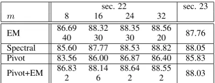
Pivot+EM 86.832 88.146 88.642 88.552 88.03 Table 1: Results on the development data (section 22) and test data (section 23) for various learning algorithms for L-PCFGs. For EM and pivot+EM experiments, the second line denotes the number of iterations required to reach the given optimal performance on development data. Results for sec-tion 23 are used with the best model for secsec-tion 22 in the cor-responding row. The results for EM and spectral are reported from Cohen et al. (2013).
in Matsuzaki et al. (2005). For the pivot algo-rithm we use multiple featuresτ1(t). . . τK(t)and
ρ1(o). . . ρL(o) over inside and outside trees, us-ing the features described by Cohen et al. (2013).
Table 1 gives the F1 accuracy on the develop-ment and test sets for the following methods:
EM: The EM algorithm as used by Matsuzaki et al. (2005) and Petrov et al. (2006).
Spectral: The spectral algorithm of Cohen et al. (2012) and Cohen et al. (2013).
Pivot: The algorithm described in this paper.
Pivot+EM: The algorithm described in this pa-per, followed by 1 or more iterations of the EM algorithm with parameters initialized by the pivot algorithm. (See section 6.3.)
For the EM and Pivot+EM algorithms, we give the number of iterations of EM required to reach optimal performance on the development data.
The results show that the EM, Spectral, and Pivot+EM algorithms all perform at a very similar level of accuracy. The Pivot+EM results show that very few EM iterations—just 2 iterations in most conditions—are required to reach optimal perfor-mance when the Pivot model is used as an ini-tializer for EM. The Pivot results lag behind the Pivot+EM results by around 2-3%, but they are close enough to optimality to require very few EM iterations when used as an initializer.
8 Experiments on the Saul and Pereira (1997) Model for Language Modeling We now describe a second set of experiments, on the Saul and Pereira (1997) model for language modeling. DefineV to be the set of words in the vocabulary. For any w1, w2 ∈ V, the Saul and
Pereira (1997) model then definesp(w2 | w1) =
Pm
[image:8.595.307.526.61.146.2]Brown NYT
m 2 4 8 16 32 128 256 test 2 4 8 16 32 128 256 test
EM 73714 59914 48819 46812 43010 3889 3658 364 92636 73339 56242 42033 36138 28435 26532 267
bi-KN +int. 408 415 271 279
tri-KN+int. 386 394 150 158
[image:9.595.85.513.61.148.2]pivot 852 718 605 559 537 426 597 560 1227 1264 896 717 738 782 886 715 pivot+EM 7582 5823 5022 4251 3741 3101 3271 357 89820 75414 55313 44115 39410 27919 29212 281
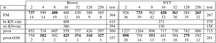
Table 2: Language model perplexity with the Brown corpus and the Gigaword corpus (New York Times portion) for the second half of the development set, and the test set. With EM and Pivot+EM, the number of iterations for EM to reach convergence is given below the perplexity. The best result for each column (for eachmvalue) is in bold. The “test” column gives perplexity results on the test set. Each perplexity calculation on the test set is done using the best model on the development set. bi-KN+int and tri-KN+int are bigram and trigram Kneser-Ney interpolated models (Kneser and Ney, 1995), using the SRILM toolkit. s(w2 | h) are parameters of the approach. The
conventional approach to estimation of the param-eters r(h | w1) ands(w2 | h) from a corpus is
to use the EM algorithm. In this section we com-pare the EM algorithm to a pivot-based method. It is straightforward to represent this model as an L-PCFG, and hence to use our implementation for estimation.
In this special case, the L-PCFG learning al-gorithm is equivalent to a simple alal-gorithm, with the following steps: 1) define the matrix Q
with entries Qw1,w2 = count(w1, w2)/N where
count(w1, w2) is the number of times that
bi-gram (w1, w2) is seen in the data, and N =
P
w1,w2count(w1, w2). Run the algorithm of
sec-tion 5.2 on Qto recover estimates ˆs(w2 | h); 2)
estimater(hˆ |w1)using the EM algorithm to
op-timize the function Pw1,w2Qw1,w2log
P hr(hˆ |
w1)ˆs(w2 | h) with respect to the ˆr parameters;
this function is concave in these parameters. We performed the language modeling experi-ments for a number of reasons. First, because in this case the L-PCFG algorithm reduces to a sim-ple algorithm, it allows us to evaluate the core ideas in the method very directly. Second, it al-lows us to test the pivot method on the very large datasets that are available for language modeling.
We use two corpora for our experiments. The first is the Brown corpus, as used by Bengio et al. (2006) in language modeling experiments. Fol-lowing Bengio et al. (2006), we use the first 800K words for training (and replace all words that ap-pear once with an UNK token), the next 200K words for development, and the remaining data (165,171 tokens) as a test set. The size of the vocabulary is 24,488 words. The second corpus we use is the New York Times portion of the Gi-gaword corpus. Here, the training set consists of 1.31 billion tokens. We use 159 million tokens for development set and 156 million tokens for test. All words that appeared less than 20 times in the
training set were replaced with the UNK token. The size of the vocabulary is 235,223 words. Un-known words in test data are ignored when calcu-lating perplexity (this is the standard set-up in the SRILM toolkit).
In our experiments we use the first half of each development set to optimize the number of itera-tions of the EM or Pivot+EM algorithms. As be-fore, Pivot+EM uses 1 or more EM steps with pa-rameter initialization from the Pivot method.
Table 2 gives perplexity results for the differ-ent algorithms. As in the parsing experimdiffer-ents, the Pivot method alone performs worse than EM, but the Pivot+EM method gives results that are com-petitive with EM. The Pivot+EM method requires fewer iterations of EM than the EM algorithm. On the Brown corpus the difference is quite dra-matic, with only 1 or 2 iterations required, as op-posed to 10 or more for EM. For the NYT cor-pus the Pivot+EM method requires more iterations (around 10 or 20), but still requires significantly fewer iterations than the EM algorithm.
On the Gigaword corpus, withm = 256, EM takes 12h57m (32 iterations at 24m18s per itera-tion) compared to 1h50m for the Pivot method. On Brown, EM takes 1m47s (8 iterations) compared to 5m44s for the Pivot method. Both the EM and pivot algorithm implementations were highly op-timized, and written in Matlab. Results at other values of m are similar. From these results the Pivot method appears to become more competitive speed-wise as the data size increases (the Giga-word corpus is more than 1,300 times larger than the Brown corpus).
9 Conclusion
References
A. Anandkumar, R. Ge, D. Hsu, S. M. Kakade, and M. Telgarsky. 2012. Tensor decompositions for learning latent-variable models. arXiv:1210.7559. S. Arora, R. Ge, and A. Moitra. 2012. Learning
topic models–going beyond SVD. InProceedings
of FOCS.
S. Arora, R. Ge, Y. Halpern, D. M. Mimno, A. Moitra, D. Sontag, Y. Wu, and M. Zhu. 2013. A practical algorithm for topic modeling with provable guaran-tees. InProceedings of ICML.
R. Bailly, A. Habrar, and F. Denis. 2010. A spectral approach for probabilistic grammatical inference on trees. InProceedings of ALT.
B. Balle, A. Quattoni, and X. Carreras. 2011. A spec-tral learning algorithm for finite state transducers. In
Proceedings of ECML.
Y. Bengio, H. Schwenk, J.-S. Sen´ecal, F. Morin, and J.-L. Gauvain. 2006. Neural probabilistic language models. InInnovations in Machine Learning, pages 137–186. Springer.
K. L. Clarkson. 2010. Coresets, sparse greedy ap-proximation, and the Frank-Wolfe algorithm. ACM Transactions on Algorithms (TALG), 6(4):63. S. B. Cohen, K. Stratos, M. Collins, D. F. Foster, and
L. Ungar. 2012. Spectral learning of latent-variable PCFGs. InProceedings of ACL.
S. B. Cohen, K. Stratos, M. Collins, D. P. Foster, and L. Ungar. 2013. Experiments with spectral learn-ing of latent-variable PCFGs. In Proceedings of
NAACL.
A. Dempster, N. Laird, and D. Rubin. 1977. Maxi-mum likelihood estimation from incomplete data via the EM algorithm. Journal of the Royal Statistical Society B, 39:1–38.
P. Dhillon, J. Rodu, M. Collins, D. P. Foster, and L. H. Ungar. 2012. Spectral dependency parsing with la-tent variables. InProceedings of EMNLP.
M. Frank and P. Wolfe. 1956. An algorithm for quadratic programming. Naval research logistics quarterly, 3(1-2):95–110.
H. Hotelling. 1936. Relations between two sets of variates. Biometrika, 28(3/4):321–377.
D. Hsu, S. M. Kakade, and T. Zhang. 2009. A spectral algorithm for learning hidden Markov models. In
Proceedings of COLT.
R. Kneser and H. Ney. 1995. Improved backing-off for m-gram language modeling. In Proceedings of
ICASSP.
E. L. Lehmann and G. Casella. 1998. Theory of Point Estimation (Second edition). Springer.
M. P. Marcus, B. Santorini, and M. A. Marcinkiewicz. 1993. Building a large annotated corpus of En-glish: The Penn treebank. Computational Linguis-tics, 19:313–330.
T. Matsuzaki, Y. Miyao, and J. Tsujii. 2005. Proba-bilistic CFG with latent annotations. InProceedings of ACL.
A. Parikh, L. Song, and E. P. Xing. 2011. A spectral algorithm for latent tree graphical models. In Pro-ceedings of ICML.
S. Petrov, L. Barrett, R. Thibaux, and D. Klein. 2006. Learning accurate, compact, and interpretable tree annotation. InProceedings of COLING-ACL. L. Saul and F. Pereira. 1997. Aggregate and
mixed-order markov models for statistical language pro-cessing. InProceedings of EMNLP.
S. Siddiqi, B. Boots, and G. Gordon. 2010. Reduced-rank hidden markov models. Journal of Machine