Hierarchical Joint Learning:
Improving Joint Parsing and Named Entity Recognition
with Non-Jointly Labeled Data
Jenny Rose Finkel and Christopher D. Manning Computer Science Department
Stanford University Stanford, CA 94305
{jrfinkel|manning}@cs.stanford.edu
Abstract
One of the main obstacles to produc-ing high quality joint models is the lack of jointly annotated data. Joint model-ing of multiple natural language process-ing tasks outperforms sprocess-ingle-task models learned from the same data, but still under-performs compared to single-task models learned on the more abundant quantities of available single-task annotated data. In this paper we present a novel model which makes use of additional single-task anno-tated data to improve the performance of a joint model. Our model utilizes a hier-archical prior to link the feature weights for shared features in several single-task models and the joint model. Experiments on joint parsing and named entity recog-nition, using the OntoNotes corpus, show that our hierarchical joint model can pro-duce substantial gains over a joint model trained on only the jointly annotated data.
1 Introduction
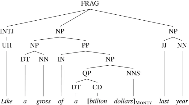
Joint learning of multiple types of linguistic struc-ture results in models which produce more consis-tent outputs, and for which performance improves across all aspects of the joint structure. Joint models can be particularly useful for producing analyses of sentences which are used as input for higher-level, more semantically-oriented systems, such as question answering and machine trans-lation. These high-level systems typically com-bine the outputs from many low-level systems, such as parsing, named entity recognition (NER) and coreference resolution. When trained sepa-rately, these single-task models can produce out-puts which are inconsistent with one another, such as named entities which do not correspond to any nodes in the parse tree (see Figure 1 for an ex-ample). Moreover, one expects that the different types of annotations should provide useful infor-mation to one another, and that modeling them
jointly should improve performance. Because a named entity should correspond to a node in the parse tree, strong evidence about either aspect of the model should positively impact the other as-pect.
However, designing joint models which actu-ally improve performance has proven challeng-ing. The CoNLL 2008 shared task (Surdeanu et al., 2008) was on joint parsing and semantic role labeling, but the best systems (Johansson and Nugues, 2008) were the ones which completely decoupled the tasks. While negative results are rarely published, this was not the first failed at-tempt at joint parsing and semantic role label-ing (Sutton and McCallum, 2005). There have been some recent successes with joint modeling. Zhang and Clark (2008) built a perceptron-based joint segmenter and part-of-speech (POS) tagger for Chinese, and Toutanova and Cherry (2009) learned a joint model of lemmatization and POS tagging which outperformed a pipelined model. Adler and Elhadad (2006) presented an HMM-based approach for unsupervised joint morpho-logical segmentation and tagging of Hebrew, and Goldberg and Tsarfaty (2008) developed a joint model of segmentation, tagging and parsing of He-brew, based on lattice parsing. No discussion of joint modeling would be complete without men-tion of (Miller et al., 2000), who trained a Collins-style generative parser (Collins, 1997) over a syn-tactic structure augmented with the template entity and template relations annotations for the MUC-7 shared task.
One significant limitation for many joint mod-els is the lack of jointly annotated data. We built a joint model of parsing and named entity recog-nition (Finkel and Manning, 2009b), which had small gains on parse performance and moderate gains on named entity performance, when com-pared with single-task models trained on the same data. However, the performance of our model, trained using the OntoNotes corpus (Hovy et al., 2006), fell short of separate parsing and named
FRAG
INTJ
UH
Like
NP
NP
DT
a
NN
gross
PP
IN
of
NP
QP
DT
a
CD
[billion
NNS
dollars]MONEY
NP
JJ
last
NN
[image:2.595.147.451.63.231.2]year
Figure 1: Example from the data where separate parse and named entity models give conflicting output.
entity models trained on larger corpora, annotated with only one type of information.
This paper addresses the problem of how to learn high-quality joint models with smaller quan-tities of jointly-annotated data that has been aug-mented with larger amounts of single-task an-notated data. To our knowledge this work is the first attempt at such a task. We use a hi-erarchical prior to link a joint model trained on jointly-annotated data with other single-task mod-els trained on single-task annotated data. The key to making this work is for the joint model to share some features with each of the single-task models. Then, the singly-annotated data can be used to in-fluence the feature weights for the shared features in the joint model. This is an important contribu-tion, because it provides all the benefits of joint modeling, but without the high cost of jointly an-notating large corpora. We applied our hierarchi-cal joint model to parsing and named entity recog-nition, and it reduced errors by over 20%on both tasks when compared to a joint model trained on only the jointly annotated data.
2 Related Work
Our task can be viewed as an instance of multi-task
learning, a machine learning paradigm in which
the objective is to simultaneously solve multiple, related tasks for which you have separate labeled training data. Many schemes for multitask learn-ing, including the one we use here, are instances of hierarchical models. There has not been much work on multi-task learning in the NLP com-munity; Daum´e III (2007) and Finkel and Man-ning (2009a) both build models for multi-domain learning, a variant on domain adaptation where there exists labeled training data for all domains and the goal is to improve performance on all of
them. Ando and Zhang (2005) utilized a multi-task learner within their semi-supervised algo-rithm to learn feature representations which were useful across a large number of related tasks. Out-side of the NLP community, Elidan et al. (2008) used an undirected Bayesian transfer hierarchy to jointly model the shapes of multiple mammal species. Evgeniou et al. (2005) applied a hier-archical prior to modeling exam scores of stu-dents. Other instances of multi-task learning in-clude (Baxter, 1997; Caruana, 1997; Yu et al., 2005; Xue et al., 2007). For a more general discus-sion of hierarchical models, we direct the reader to Chapter 5 of (Gelman et al., 2003) and Chapter 12 of (Gelman and Hill, 2006).
3 Hierarchical Joint Learning
In this section we will discuss the main con-tribution of this paper, our hierarchical joint model which improves joint modeling perfor-mance through the use of single-task models which can be trained on singly-annotated data. Our experiments are on a joint parsing and named entity task, but the technique is more general and only requires that the base models (the joint model and single-task models) share some features. This section covers the general technique, and we will cover the details of the parsing, named entity, and joint models that we use in Section 4.
3.1 Intuitive Overview
PARSE JOINT NER
µ
θ∗ σ∗
θp σp
Dp
θj σj
Dj
θn σn
[image:3.595.75.281.59.222.2]Dn
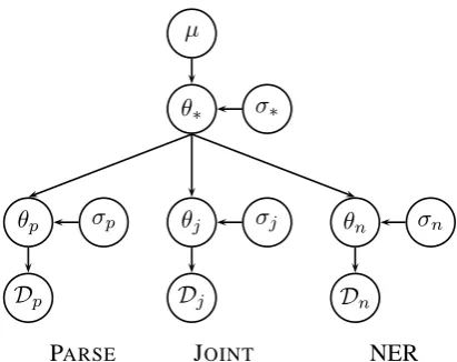
Figure 2: A graphical representation of our hierar-chical joint model. There are separate base models for just parsing, just NER, and joint parsing and NER. The parameters for these models are linked via a hierarchical prior.
Each model has its own set of parameters (feature weights). However, parameters for the features which are shared between the single-task models and the joint model are able to influence one an-other via a hierarchical prior. This prior encour-ages the learned weights for the different models to be similar to one another. After training has been completed, we retain only the joint model’s parameters. Our resulting joint model is of higher quality than a comparable joint model trained on only the jointly-annotated data, due to all of the ev-idence provided by the additional single-task data.
3.2 Formal Model
We have a set M of three base models: a parse-only model, an NER-only model and a joint model. These have corresponding log-likelihood functionsLp(Dp;θp),Ln(Dn;θn), and Lj(Dj;θj), where theDs are the training data for each model, and theθs are the model-specific pa-rameter (feature weight) vectors. These likelihood functions do not include priors over the θs. For representational simplicity, we assume that each of these vectors is the same size and corresponds to the same ordering of features. Features which don’t apply to a particular model type (e.g., parse features in the named entity model) will always be zero, so their weights have no impact on that model’s likelihood function. Conversely, allowing the presence of those features in models for which they do not apply will not influence their weights in the other models because there will be no evi-dence about them in the data. These three models are linked by a hierarchical prior, and their fea-ture weight vectors are all drawn from this prior.
The parametersθ∗for this prior have the same di-mensionality as the model-specific parametersθm and are drawn from another, top-level prior. In our case, this top-level prior is a zero-mean Gaussian.1 The graphical representation of our hierarchical model is shown in Figure 2. The log-likelihood of this model is
Lhier-joint(D;θ) = (1)
X
m∈M
Lm(Dm;θm)−
X
i
(θm,i−θ∗,i)2
2σ2
m
!
−X i
(θ∗,i−µi)2
2σ2
∗
The first summation in this equation computes the log-likelihood of each model, using the data and parameters which correspond to that model, and the prior likelihood of that model’s parameters, based on a Gaussian prior centered around the top-level, non-model-specific parameters θ∗, and with model-specific variance σm. The final sum-mation in the equation computes the prior likeli-hood of the top-level parametersθ∗according to a Gaussian prior with varianceσ∗and meanµ (typ-ically zero). This formulation encourages each base model to have feature weights similar to the top-level parameters (and hence one another).
The effects of the variancesσm andσ∗ warrant some discussion.σ∗has the familiar interpretation of dictating how much the model “cares” about feature weights diverging from zero (or µ). The model-specific variances,σm, have an entirely dif-ferent interpretation. They dictate how how strong the penalty is for the domain-specific parameters to diverge from one another (via their similarity to
θ∗). Whenσm are very low, then they are encour-aged to be very similar, and taken to the extreme this is equivalent to completely tying the parame-ters between the tasks. When σm are very high, then there is less encouragement for the parame-ters to be similar, and taken to the extreme this is equivalent to completely decoupling the tasks.
We need to compute partial derivatives in or-der to optimize the model parameters. The partial derivatives for the parameters for each base model
mare given by:
∂Lhier(D;θ) ∂θm,i
= ∂Lm(Dm, θm) ∂θm,i
−θm,i−θ∗,i
σ2d
(2) where the first term is the partial derivative ac-cording to the base model, and the second term is
1Though we use a zero-mean Gaussian prior, this
top-level prior could take many forms, including anL1prior, or
the prior centered around the top-level parameters. The partial derivatives for the top level parameters
θ∗are:
∂Lhier(D;θ) ∂θ∗,i
= X
m∈M
θ∗,i−θm,i
σ2
m
!
−θ∗,i−µi
σ2
∗ (3) where the first term relates to how far each model-specific weight vector is from the top-level param-eter values, and the second term relates how far each top-level parameter is from zero.
When a model has strong evidence for a feature, effectively what happens is that it pulls the value of the top-level parameter for that feature closer to the model-specific value for it. When it has little or no evidence for a feature then it will be pulled in the direction of the top-level parameter for that feature, whose value was influenced by the models which have evidence for that feature.
3.3 Optimization with Stochastic Gradient Descent
Inference in joint models tends to be slow, and of-ten requires the use of stochastic optimization in order for the optimization to be tractable. L-BFGS and gradient descent, two frequently used numer-ical optimization algorithms, require computing the value and partial derivatives of the objective function using the entire training set. Instead, we use stochastic gradient descent. It requires a stochastic objective function, which is meant to be a low computational cost estimate of the real ob-jective function. In most NLP models, such as lo-gistic regression with a Gaussian prior, computing the stochastic objective function is fairly straight-forward: you compute the model likelihood and partial derivatives for a randomly sampled subset of the training data. When computing the term for the prior, it must be rescaled by multiplying its value and derivatives by the proportion of the training data used. The stochastic objective func-tion, whereD ⊆ Db is a randomly drawn subset of the full training set, is given by
Lstoch(D;θ) =Lorig(Db;θ)− |D|b |D|
X
i
(θ∗,i)2
2σ2
∗ (4) This is a stochastic function, and multiple calls to it with the same D and θ will produce different values because Db is resampled each time. When designing a stochastic objective function, the crit-ical fact to keep in mind is that the summed values and partial derivatives for any split of the data need to be equal to that of the full dataset. In practice,
stochastic gradient descent only makes use of the partial derivatives and not the function value, so we will focus the remainder of the discussion on how to rescale the partial derivatives.
We now describe the more complicated case of stochastic optimization with a hierarchical ob-jective function. For the sake of simplicity, let us assume that we are using a batch size of one, meaning |D|b = 1 in the above equation. Note that in the hierarchical model, each datum (sen-tence) in each base model should be weighted equally, so whichever dataset is the largest should be proportionally more likely to have one of its data sampled. For the sampled datumd, we then compute the function value and partial derivatives with respect to the correct base model for that da-tum. When we rescale the model-specific prior, we rescale based on the number of data in that model’s training set, not the total number of data in all the models combined. Having uniformly randomly drawn datum d ∈ Sm∈MDm, let m(d) ∈ M tell us to which model’s training data the datum belongs. The stochastic partial derivatives will equal zero for all model parameters θm such that
m6=m(d), and forθm(d)it becomes: ∂Lhier-stoch(D;θ)
∂θm(d),i = (5)
∂Lm(d)({d};θm(d))
∂θm(d),i −
1
|Dm(d)|
θ
m(d),i−θ∗,i
σ2d
Now we will discuss the stochastic partial deriva-tives with respect to the top-level parameters θ∗, which requires modifying Equation 3. The first term in that equation is a summation over all the models. In the stochastic derivative we only perform this computation for the datum’s model
m(d), and then we rescale that value based on the number of data in that datum’s model|Dm(d)|. The
second term in that equation is rescaled by the
to-tal number of data in all models combined. The
stochastic partial derivatives with respect toθ∗ be-come:
∂Lhier-stoch(D;θ) ∂θ∗,i
= (6)
1
|Dm(d)|
θ
∗,i−θm(d),i
σ2
m
− P 1
m∈M |Dm|
θ
∗,i
σ2
∗
where for conciseness we omit µ under the as-sumption that it equals zero.
B-PER
Hilary
I-PER
Clinton
O
visited
B-GPE
Haiti
O
.
(a)
PER
Hilary Clinton
O
visited
GPE
Haiti
O
.
(b)
ROOT
PER
PER-i
Hilary
PER-i
Clinton
O
visited
GPE
GPE-i
Haiti
O
.
[image:5.595.80.272.74.372.2](c)
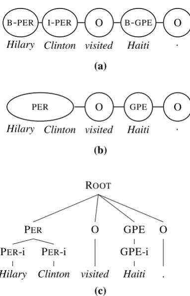
Figure 3: A linear-chain CRF (a) labels each word, whereas a semi-CRF (b) labels entire entities. A semi-CRF can be represented as a tree (c), where i indicates an internal node for an entity.
slower to compute because it required summing over the parameter vectors for all base models in-stead of just the vector for the datum’s model.
When using a batch size larger than one, you compute the given functions for each datum in the batch and then add them together.
4 Base Models
Our hierarchical joint model is composed of three separate models, one for just named entity recog-nition, one for just parsing, and one for joint pars-ing and named entity recognition. In this section we will review each of these models individually.
4.1 Semi-CRF for Named Entity Recognition
For our named entity recognition model we use a semi-CRF (Sarawagi and Cohen, 2004; Andrew, 2006). Semi-CRFs are very similar to the more popular linear-chain CRFs, but with several key advantages. Semi-CRFs segment and label the text simultaneously, whereas a linear-chain CRF will only label each word, and segmentation is im-plied by the labels assigned to the words. When
doing named entity recognition, a semi-CRF will have one node for each entity, unlike a regular CRF which will have one node for each word.2 See Figure 3a-b for an example of a semi-CRF and a linear-chain CRF over the same sentence. Note that the entity Hilary Clinton has one node in the semi-CRF representation, but two nodes in the linear-chain CRF. Because different segmen-tations have different model structures in a semi-CRF, one has to consider all possible structures (segmentations) as well as all possible labelings. It is common practice to limit segment length in order to speed up inference, as this allows for the use of a modified version of the forward-backward algorithm. When segment length is not restricted, the inference procedure is the same as that used in parsing (Finkel and Manning, 2009c).3 In this work we do not enforce a length restriction, and directly utilize the fact that the model can be trans-formed into a parsing model. Figure 3c shows a parse tree representation of a semi-CRF.
While a linear-chain CRF allows features over adjacent words, a semi-CRF allows them over ad-jacent segments. This means that a semi-CRF can utilize all features used by a linear-chain CRF, and can also utilize features over entire segments, such as First National Bank of New York City, instead of just adjacent words like First National and Bank
of. Letybe a vector representing the labeling for an entire sentence. yiencodes the label of theith segment, along with the span of words the seg-ment encompasses. Letθbe the feature weights, and f(s, yi, yi−1) the feature function over
adja-cent segmentsyiandyi−1in sentences.4 The log
likelihood of a semi-CRF for a single sentencesis given by:
L(y|s;θ) = 1 Zs
|y| X
i=1
exp{θ·f(s, yi, yi−1)} (7)
The partition function Zs serves as a normalizer. It requires summing over the setysof all possible segmentations and labelings for the sentences:
Zs =
X
y∈ys
|y| X
i=1
exp{θ·f(s, yi, yi−1)} (8)
2
Both models will have one node per word for non-entity words.
3While converting a semi-CRF into a parser results in
much slower inference than a linear-chain CRF, it is still sig-nificantly faster than a treebank parser due to the reduced number of labels.
4There can also be features over single entities, but these
FRAG
INTJ
UH
Like
NP
NP
DT
a
NN
gross
PP
IN
of
NP-MONEY
QP-MONEY-i
DT-MONEY-i
a
CD-MONEY-i
billion
NNS-MONEY-i
dollars
NP
JJ
last
NN
[image:6.595.106.497.63.232.2]year
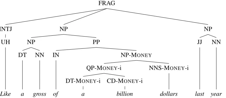
Figure 4: An example of a sentence jointly annotated with parse and named entity information. Named entities correspond to nodes in the tree, and the parse label is augmented with the named entity informa-tion.
Because we use a tree representation, it is easy to ensure that the features used in the NER model are identical to those in the joint parsing and named entity model, because the joint model (which we will discuss in Section 4.3) is also based on a tree representation where each entity corresponds to a single node in the tree.
4.2 CRF-CFG for Parsing
Our parsing model is the discriminatively trained, conditional random field-based context-free gram-mar parser (CRF-CFG) of (Finkel et al., 2008). The relationship between a CRF-CFG and a PCFG is analogous to the relationship between a linear-chain CRF and a hidden Markov model (HMM) for modeling sequence data. Let t be a com-plete parse tree for sentence s, and each lo-cal subtree r ∈ t encodes both the rule from the grammar, and the span and split informa-tion (e.g NP(7,9) →JJ(7,8)NN(8,9) which covers
the last two words in Figure 1). The feature func-tion f(r, s) computes the features, which are de-fined over a local subtree r and the words of the sentence. Let θbe the vector of feature weights. The log-likelihood of treetover sentencesis:
L(t|s;θ) = 1 Zs
X
r∈t
exp{θ·f(r, s)} (9)
To compute the partition function Zs, which serves to normalize the function, we must sum over τ(s), the set of all possible parse trees for sentences. The partition function is given by:
Zs=
X
t′∈τ(s)
X
r∈t′
exp{θ·f(r, s)}
We also need to compute the partial derivatives which are used during optimization. Let fi(r, s)
be the value of feature i for subtree r over sen-tence s, and let Eθ[fi|s]be the expected value of featureiin sentences, based on the current model parametersθ. The partial derivatives of θare then given by
∂L
∂θi
= X
(t,s)∈D
X
r∈t
fi(r, s)
−Eθ[fi|s]
!
(10) Just like with a linear-chain CRF, this equation will be zero when the feature expectations in the model equal the feature values in the training data. A variant of the inside-outside algorithm is used to efficiently compute the likelihood and partial derivatives. See (Finkel et al., 2008) for details.
4.3 Joint Model of Parsing and Named Entity Recognition
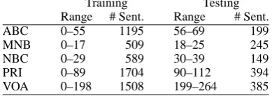
ad-Training Testing Range # Sent. Range # Sent.
ABC 0–55 1195 56–69 199
MNB 0–17 509 18–25 245
NBC 0–29 589 30–39 149
PRI 0–89 1704 90–112 394
[image:7.595.84.279.65.134.2]VOA 0–198 1508 199–264 385
Table 1: Training and test set sizes for the five datasets in sentences. The file ranges refer to the numbers within the names of the original OntoNotes files.
ditional joint rules which are composed by adding named entity information to existing parse rules. Because the grammars are based on the observed data, and the two models have different data, they will have somewhat different grammars. In our hi-erarchical joint model, we added all observed rules from the joint data (stripped of named entity infor-mation) to the parse-only grammar, and we added all observed rules from the parse-only data to the grammar for the joint model, and augmented them with named entity information in the same manner as the rules observed in the joint data.
Earlier we said that the NER-only model uses identical named entity features as the joint model (and similarly for the parse-only model), but this is not quite true. They use identical feature
tem-plates, such as word, but different realizations
of those features will occur with the different datasets. For instance, the NER-only model may have word=Nigel as a feature, but because Nigel never occurs in the joint data, that feature is never manifested and no weight is learned for it. We deal with this similarly to how we dealt with the gram-mar: if a named entity feature occurs in either the joint data or the NER-only data, then both mod-els will learn a weight for that feature. We do the same thing for the parse features. This modeling decision gives the joint model access to potentially useful features to which it would not have had ac-cess if it were not part of the hierarchical model.5
5 Experiments and Discussion
We compared our hierarchical joint model to a reg-ular (non-hierarchical) joint model, and to parse-only and NER-parse-only models. Our baseline ex-periments were modeled after those in (Finkel and Manning, 2009b), and while our results were not identical (we updated to a newer release of the data), we had similar results and found the same general trends with respect to how the joint
5In the non-hierarchical setting, you could include those
features in the optimization, but, because there would be no evidence about them, their weights would be zero due to reg-ularization.
model improved on the single models. We used OntoNotes 3.0 (Hovy et al., 2006), and made the same data modifications as (Finkel and Manning, 2009b) to ensure consistency between the parsing and named entity annotations. Table 2 has our complete set of results, and Table 1 gives the num-ber of training and test sentences. For each sec-tion of the data (ABC, MNB, NBC, PRI, VOA) we ran experiments training a linear-chain CRF on only the named entity information, a CRF-CFG parser on only the parse information, a joint parser and named entity recognizer, and our hierarchi-cal model. For the hierarchihierarchi-cal model, we used the CNN portion of the data (5093sentences) for the extra named entity data (and ignored the parse trees) and the remaining portions combined for the extra parse data (and ignored the named entity an-notations). We used σ∗ = 1.0 and σm = 0.1, which were chosen based on early experiments on development data. Small changes to σm do not appear to have much influence, but larger changes do. We similarly decided how many iterations to run stochastic gradient descent for (20) based on early development data experiments. We did not run this experiment on the CNN portion of the data, because the CNN data was already being used as the extra NER data.
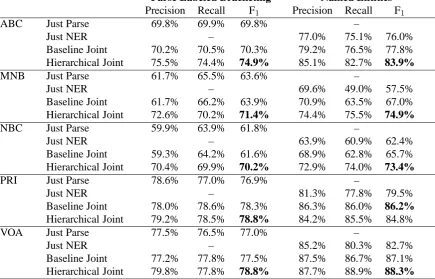
As Table 2 shows, the hierarchical model did substantially better than the joint model overall, which is not surprising given the extra data to which it had access. Looking at the smaller cor-pora (NBC and MNB) we see the largest gains, with both parse and NER performance improving by about 8% F1. ABC saw about a 6%gain on both tasks, and VOA saw a1%gain on both. Our one negative result is in the PRI portion: parsing improves slightly, but NER performance decreases by almost 2%. The same experiment on develop-ment data resulted in a performance increase, so we are not sure why we saw a decrease here. One general trend, which is not surprising, is that the hierarchical model helps the smaller datasets more than the large ones. The source of this is two-fold: lower baselines are generally easier to im-prove upon, and the larger corpora had less singly-annotated data to provide improvements, because it was composed of the remaining, smaller, sec-tions of OntoNotes. We found it interesting that the gains tended to be similar on both tasks for all datasets, and believe this fact is due to our use of roughly the same amount of singly-annotated data for both parsing and NER.
Parse Labeled Bracketing Named Entities
Precision Recall F1 Precision Recall F1
ABC Just Parse 69.8% 69.9% 69.8% –
Just NER – 77.0% 75.1% 76.0%
Baseline Joint 70.2% 70.5% 70.3% 79.2% 76.5% 77.8% Hierarchical Joint 75.5% 74.4% 74.9% 85.1% 82.7% 83.9%
MNB Just Parse 61.7% 65.5% 63.6% –
Just NER – 69.6% 49.0% 57.5%
Baseline Joint 61.7% 66.2% 63.9% 70.9% 63.5% 67.0% Hierarchical Joint 72.6% 70.2% 71.4% 74.4% 75.5% 74.9%
NBC Just Parse 59.9% 63.9% 61.8% –
Just NER – 63.9% 60.9% 62.4%
Baseline Joint 59.3% 64.2% 61.6% 68.9% 62.8% 65.7% Hierarchical Joint 70.4% 69.9% 70.2% 72.9% 74.0% 73.4%
PRI Just Parse 78.6% 77.0% 76.9% –
Just NER – 81.3% 77.8% 79.5%
Baseline Joint 78.0% 78.6% 78.3% 86.3% 86.0% 86.2%
Hierarchical Joint 79.2% 78.5% 78.8% 84.2% 85.5% 84.8%
VOA Just Parse 77.5% 76.5% 77.0% –
Just NER – 85.2% 80.3% 82.7%
[image:8.595.79.515.71.350.2]Baseline Joint 77.2% 77.8% 77.5% 87.5% 86.7% 87.1% Hierarchical Joint 79.8% 77.8% 78.8% 87.7% 88.9% 88.3%
Table 2: Full parse and NER results for the six datasets. Parse trees were evaluated using evalB, and named entities were scored using micro-averaged F-measure (conlleval).
get the most similar annotated data available – data which was annotated by the same annotators, and all of which is broadcast news – these are still dif-ferent domains. While this is likely to have a nega-tive effect on results, we also believe this scenario to be a more realistic than if it were to also be data drawn from the exact same distribution.
6 Conclusion
In this paper we presented a novel method for improving joint modeling using additional data which has not been labeled with the entire joint structure. While conventional wisdom says that adding more training data should always improve performance, this work is the first to our knowl-edge to incorporate singly-annotated data into a joint model, thereby providing a method for this additional data, which cannot be directly used by the non-hierarchical joint model, to help improve joint modeling performance. We built single-task models for the non-jointly labeled data, designing those single-task models so that they have features in common with the joint model, and then linked all of the different single-task and joint models via a hierarchical prior. We performed experi-ments on joint parsing and named entity recogni-tion, and found that our hierarchical joint model substantially outperformed a joint model which
was trained on only the jointly annotated data. Future directions for this work include automat-ically learning the variances,σmandσ∗ in the hi-erarchical model, so that the degree of information sharing between the models is optimized based on the training data available. We are also interested in ways to modify the objective function to place more emphasis on learning a good joint model, in-stead of equally weighting the learning of the joint and single-task models.
Acknowledgments
Many thanks to Daphne Koller for discussions which led to this work, and to Richard Socher for his assistance and input. Thanks also to our anonymous reviewers and Yoav Goldberg for use-ful feedback on an earlier draft of this paper.
References
Meni Adler and Michael Elhadad. 2006. An unsupervised morpheme-based hmm for hebrew morphological disam-biguation. In Proceedings of the 21st International Con-ference on Computational Linguistics and the 44th annual meeting of the Association for Computational Linguistics, pages 665–672, Morristown, NJ, USA. Association for Computational Linguistics.
Rie Kubota Ando and Tong Zhang. 2005. A high-performance semi-supervised learning method for text chunking. In ACL ’05: Proceedings of the 43rd Annual Meeting on Association for Computational Linguistics, pages 1–9, Morristown, NJ, USA. Association for Com-putational Linguistics.
Galen Andrew. 2006. A hybrid markov/semi-markov con-ditional random field for sequence segmentation. In Pro-ceedings of the Conference on Empirical Methods in Nat-ural Language Processing (EMNLP 2006).
J. Baxter. 1997. A bayesian/information theoretic model of learning to learn via multiple task sampling. In Machine Learning, volume 28.
R. Caruana. 1997. Multitask learning. In Machine Learning, volume 28.
Michael Collins. 1997. Three generative, lexicalised models for statistical parsing. In ACL 1997.
Hal Daum´e III. 2007. Frustratingly easy domain adaptation. In Conference of the Association for Computational Lin-guistics (ACL), Prague, Czech Republic.
Gal Elidan, Benjamin Packer, Geremy Heitz, and Daphne Koller. 2008. Convex point estimation using undirected bayesian transfer hierarchies. In UAI 2008.
T. Evgeniou, C. Micchelli, and M. Pontil. 2005. Learning multiple tasks with kernel methods. In Journal of Machine Learning Research.
Jenny Rose Finkel and Christopher D. Manning. 2009a. Hi-erarchical bayesian domain adaptation. In Proceedings of the North American Association of Computational Lin-guistics (NAACL 2009).
Jenny Rose Finkel and Christopher D. Manning. 2009b. Joint parsing and named entity recognition. In Proceedings of the North American Association of Computational Lin-guistics (NAACL 2009).
Jenny Rose Finkel and Christopher D. Manning. 2009c. Nested named entity recognition. In Proceedings of EMNLP 2009.
Jenny Rose Finkel, Alex Kleeman, and Christopher D. Man-ning. 2008. Efficient, feature-based conditional random field parsing. In ACL/HLT-2008.
Andrew Gelman and Jennifer Hill. 2006. Data Analysis Us-ing Regression and Multilevel/Hierarchical Models. Cam-bridge University Press.
A. Gelman, J. B. Carlin, H. S. Stern, and Donald D. B. Rubin. 2003. Bayesian Data Analysis. Chapman & Hall. Yoav Goldberg and Reut Tsarfaty. 2008. A single
genera-tive model for joint morphological segmentation and syn-tactic parsing. In Proceedings of ACL-08: HLT, pages 371–379, Columbus, Ohio, June. Association for Compu-tational Linguistics.
Eduard Hovy, Mitchell Marcus, Martha Palmer, Lance Ramshaw, and Ralph Weischedel. 2006. Ontonotes: The 90% solution. In HLT-NAACL 2006.
Richard Johansson and Pierre Nugues. 2008. Dependency-based syntactic-semantic analysis with propbank and nombank. In CoNLL ’08: Proceedings of the Twelfth Conference on Computational Natural Language Learn-ing, pages 183–187, Morristown, NJ, USA. Association for Computational Linguistics.
Scott Miller, Heidi Fox, Lance Ramshaw, and Ralph Weischedel. 2000. A novel use of statistical parsing to extract information from text. In In 6th Applied Natural Language Processing Conference, pages 226–233. Sunita Sarawagi and William W. Cohen. 2004. Semi-markov
conditional random fields for information extraction. In In Advances in Neural Information Processing Systems 17, pages 1185–1192.
Mihai Surdeanu, Richard Johansson, Adam Meyers, Llu´ıs M`arquez, and Joakim Nivre. 2008. The CoNLL-2008 shared task on joint parsing of syntactic and semantic dependencies. In Proceedings of the 12th Conference on Computational Natural Language Learning (CoNLL), Manchester, UK.
Charles Sutton and Andrew McCallum. 2005. Joint pars-ing and semantic role labelpars-ing. In Conference on Natural Language Learning (CoNLL).
Kristina Toutanova and Colin Cherry. 2009. A global model for joint lemmatization and part-of-speech prediction. In Proceedings of the Joint Conference of the 47th Annual Meeting of the ACL and the 4th International Joint Con-ference on Natural Language Processing of the AFNLP, pages 486–494, Suntec, Singapore, August. Association for Computational Linguistics.
Ya Xue, Xuejun Liao, Lawrence Carin, and Balaji Krishna-puram. 2007. Multi-task learning for classification with dirichlet process priors. J. Mach. Learn. Res., 8.
Kai Yu, Volker Tresp, and Anton Schwaighofer. 2005. Learn-ing gaussian processes from multiple tasks. In ICML ’05: Proceedings of the 22nd international conference on Ma-chine learning.