Munich Personal RePEc Archive
Valuing Inputs Under Supply
Uncertainty : The Bayesian Shapley
Value
Pongou, Roland and Tondji, Jean-Baptiste
University of Ottawa, University of Ottawa
25 October 2016
Online at
https://mpra.ub.uni-muenchen.de/74747/
Valuing Inputs Under Supply Uncertainty : The
Bayesian Shapley Value
∗
Roland Pongou
†and Jean-Baptiste Tondji
‡October 25, 2016
Abstract
We consider the problem of valuing inputs in a production environment in which input supply is uncertain. Inputs can be workers in a firm, risk factors for a disease, securities in a financial market, or nodes in a networked economy. Each input takes its values from a finite set, and uncertainty is modeled as a probability distribution over this set. First, we provide an axiomatic solution to our valuation problem, defining three intuitive axioms which we use to uniquely characterize a valuation scheme that we call the
a priori Shapley value.
Second, we solve the problem of valuing inputs a posteriori – that is, after observing output. This leads to theBayesian Shapley value.
Third, we consider the problem of rationalizing uncertainty when the inputs are rational workers supplying labor in a non-cooperative production game in which payoffs are given by the Shapley wage function. We find that probability distributions over labor supply that can be supported as mixed strategy Nash equilibria always exist. We also provide an intuitive condition under which we prove the existence of a pure strategy Nash equilibrium. We present several applications of our theory to real-life situations.
JEL classification codes: C70, D20, D80, J30.
Keywords: Input valuation, uncertainty,a prioriShapley value, Bayesian Shapley value, rationalizability.
1
Introduction
In this paper, we consider the problem of valuing inputs in a production environment where input supply is uncertain. Each input is a discrete variable taking values from a finite set, and uncertainty is formalized as a probability distribution over this set, viewed as a sample space. A production function maps each input profile to a measurable output. Given the uncertainty characterizing the supply of inputs, the level of output cannot be knowna priori. We answer the following questions:
1. What value can we attach to each inputa priori?
2. Assume an output level is realized. What value can we attach to each inputa posteriori?
3. Assume that inputs are “rational” production factors (e.g., workers) choosing their effort level in a non-cooperative manner. Can certain probability distributions over effort levels be rationalized?
The production environment described above fits many real-life situations, as illustrated by the following examples.
Example 1. (Valuing workers’ unobserved abilities and skills) The production of a certain good
requires n types of skills and n workers, with each worker supplying a different skill. Output is generated
by a production function f that depends on the ability of each worker in the skill that she possesses. A
worker’s ability level belongs to the finite set T = {0,1,2}, where 0 means low ability, 1 medium ability, and2 high ability. The ability of a worker is not known, but the distribution of ability for each skill type in the population is known. If we assume that each worker is randomly chosen from the pool of workers who
possess her skill type, the answer to question (1) above will determine the a priori contribution of each skill
type in the production process. Following the realization of an output level, we answer question (2) by first
uncovering the posterior distributions of abilities among the selected workers, and using this information, we
determine the effective contribution of each skill type to the production of the output. Finally, given that the
ability distribution is exogenous in this particular example, question (3) is irrelevant.
Example 2. (Assessing the risk factors of a disease) A disease (e.g., diabetes) is caused by a set
of risks factors (e.g., obesity, low fruit and vegetable intake, lack of physical activity, smoking, high blood
pressure). The level (or severity) of each risk factoribelongs to a finite sample spaceTi, and the production
function of the disease,f, maps each risk profile to the probability with which an individual with such a risk
profile will develop the disease. Assuming that each risk factor has a probability distribution in the population,
the answer to question (1) will reveal the total contribution of each risk factor to the prevalence of the disease
in the population. Assume that the prevalence of the disease is observed in a subgroup of the population
for which no information on the distribution of risk factors is available. Then one can determine the total
Example 3. (Rationalizing random and non-random labor supply in a firm) A firm employs n
workers. Each worker supplies labor in discrete units (zero hours, one hour, two hours, and so on) up to a
maximum amount – say, nine hours per day. A production technology f maps each profile of hours worked
to a real number output that is shared among the workers according to the Shapley wage function (see below).
Unlike in Example 1 and Example 2, we assume that there is no uncertainty a priori regarding the number
of hours of work supplied by each worker. We are interested in whether there exist probability distributions
over the number of worked hours that can be rationalized as Nash equilibria.
In this paper, we develop a theory to answer these questions. Our model of an uncertain production environment is a tuple (N,(Ti)i∈N, f, π), whereN is a finite set of inputs,Ti a finite set of values that can
be taken by input i, f a production function that maps each input profile to a real number output, and
π = (πi)i∈N a profile of probability distributions – with πi being the probability distribution of input i
over the setTi. We take an axiomatic approach to answer the question of how to value each inputa priori.
We define three intuitive axioms of a valuation scheme –probabilistic symmetry,probabilistic efficiency, and
marginality – and show that one and only one valuation scheme satisfies all three axioms. We call this scheme thea priori Shapley value. These axioms generalize to our environment the traditional axioms of symmetry, efficiency, and marginality that characterize the classical Shapley value (Shapley (1953), Young (1985)). In the classical environment, it is assumed that for each inputi∈N,Ti={0,1},πi(0) = 0, andπi(1) = 1. That
is, each agent has only two options – “work” and “not work” – and all agents choose to work.1 Clearly, our
environment is more general, as players have more choices and may not all choose the same action. Another distinctive feature of our environment is to assume uncertainty in the supply of inputs, which makes this environment more realistic.
Now, assuming that a levelY of the output is realized, we answer the question of how to value each input
a posteriori. We use a Bayesian updating procedure to determine theposterior probability distributions of inputs, P(.|Y), which we use to obtain the Bayesian Shapley value. The Bayesian Shapley value therefore determines the contribution of each input to the realized output Y. This value is the unique valuation procedure that satisfies modified versions of the aforementioned axioms that take into account the updated profile of probability distributionsP(.|Y). This is because our characterization of thea prioriShapley value is valid for any profile of probability distributionsπ. Importantly, we also show that averaging the Bayesian Shapley value over the set of realizable outputs yields thea priori Shapley value.
In certain situations, such as when a worker’s performance depends on weather conditions, the probability distribution of each input might be exogenous. But there also exist situations in which inputs – viewed as rational agents – may choose probability distributions that maximize their payoffs. We therefore answer the question of whether such probability distributions exist in our setting. We assume a production environment (N,(Ti)i∈N, f) free of any exogenous profile of probability distributions of inputs. We additionally assume
1
that the payoff to each worker at each input profile is determined by the value of the Shapley wage function at that profile.2 These assumptions lead to a finite non-cooperative game (N,Qn
i=1
Ti,(ui)i∈N) where ui is
the payoff function of player i given by the Shapley wage function under the technology f. A profile of probability distributions πis rationalizable if it is a Nash equilibrium of the game (N,Qn
i=1
Ti,(ui)i∈N). We
prove the existence of rationalizable probability distributions. This proof simply derives from the proof of the existence of a mixed strategy equilibrium in any finite non-cooperative game (Nash (1951)). We also find a natural condition that guarantees the existence of a pure strategy Nash equilibrium. This result states that if the production function exhibits positive interaction or complementarity, there exists a rationalizable probability distribution in which each agent assigns the maximum weight to the highest effort level.
In addition to the applications mentioned above, we provide an application to contagion in a networked economy in which self-interested agents freely form and sever bilateral links. Rationality is captured by a certain equilibrium notion (e.g., pairwise stability, stochastic stability, etc.). We apply thea priori Shapley value to determine the expected contribution of each agent (or node) to the spread of a random infection that might hit the economy. This application assumes that only equilibrium networks can form. Second, given an observed contagion level, we are able to determine the contribution of each agent to this outcome using the Bayesian Shapley value. In particular, this application is implemented for fidelity economies (see Pongou (2010), Pongou and Serrano (2013)) to determine individual responsibilities in the spread of a random infectiona priori anda posteriori. It turns out that these measures can also be used to assess the expected and the actual centrality of agents in an economy. While the expected centrality of an agent depends on his/her desired number of partners, his/her actual centrality depends on the realized equilibrium network, and both can be very different.
To the best of our knowledge, we are the first to propose an axiomatic solution to the problem of input valuation in an uncertain production environment. We are also the first to introduce the notions of thea priori
Shapley value and the Bayesian Shapley value. In addition, our environment may apply to several real-life situations as shown in the examples above. Theoretical and empirical works on the general transferable-utility environment assume no uncertainty in the supply of inputs (see, e.g., Roth (1989) and Serrano (2013) for an excellent account of the different generalizations of the classical Shapley value). Our model differs in assuming that exogenous shocks may affect the supply of inputs.
Our work is related to papers that have generalized the Shapley value to games in which players have multiple options (see, e.g., Freixas (2005), Hsiao and Raghavan (1993)). We depart from these papers by incorporating uncertainty. Our axiomatic approach is also different. Also, our scope is different in that we introduce a non-cooperative production game with Shapley payoffs and prove the existence of mixed and pure strategy Nash equilibria. Another distinctive feature of our work is the application of thea priori and
2
The value of the Shapley wage function at an input profilex∈T =
n
Q
i=1
Ti is given by thea prioriShapley value of the
uncertain production environment (N,(Ti)i∈N, f, π) where each component ofx receives a weight of 1 (that is, each agenti
the Bayesian Shapley values to networked economies, with a particular emphasis on fidelity networks. The rest of this paper is organized as follows. Section 2 introduces the uncertain production environment and other preliminary concepts. Section 3 proposes an axiomatic solution to the valuation problema priori. Section 4 introduces the Bayesian Shapley value as a solution to the valuation problema posteriori. Section 5 is devoted to the analysis of the existence of rationalizable probability distributions in a non-cooperative production game under the Shapley wage function. In Section 6, we provide a specific application of our analysis to networked economies. Section 7 concludes. All proofs are collected in the appendix.
2
Uncertain Production Environment
An uncertain production environment is modeled as a tupleP= (N,(Ti)i∈N, f, π) whereN ={1,2, ..., n}is
a finite set of inputs of cardinality n,Ti={0,1,2, ..., ti} is a finite set of values an inputi can take,f is a
production function which maps an input profilex= (x1, ..., xn)∈T = n
Q
i=1
Ti to a real number outputf(x),
andπ= (πi)i∈N is a profile of probability distributions of inputs. More formally, for each inputi, we have:
πi : Ti −→ [0,1]
xi 7−→ πi(xi) with P xi∈Ti
πi(xi) = 1.
Throughout the paper, we assume f(0,0, ...,0) = 0, which means that if all inputs are inactive, there will be no output. The interpretation of inputs depends on the production environment being analyzed. For example, an input level may be the number of hours supplied by a worker in a firm, the unobserved ability of a worker, the level of effort that a student puts into a class project, or the severity of a risk factor for a disease. Note that the elements of each input setTi need not be interpreted as numbers – they can simply
be viewed as labels. For instance,Ti might represent the different types of jobs to which worker i can be
assigned in a firm; in this case,Ti is not necessarily an ordered set. We also note that, for each inputi, Ti
might represent a different set of objects (that is, action 1 in setT1 might not represent the same object as
action 1 in setT2).
We denote byπ(x) the probability of the realization of an input profilex∈T. Interestingly, if we assume that the input variables are independently distributed, the probability of the realization of an input profile
x∈T is:
π(x) = Q
i∈N
πi(xi).
3
A Priori
Shapley Value
Given a production environment P = (N,(Ti)i∈N, f, π), what is the contribution a priori of each input
factor to output production? Answering this question is important in several contexts. It may reveal the pay a worker employed by a firm can expect to receive from the firm’s revenue, or the fraction of the prevalence of a disease that can be attributed to a given risk factor. We propose an axiomatic solution to this problem. We introduce three intuitive axioms inspired by the works of Shapley (1953) and Young (1985), and use them to uniquely characterize a valuation procedure that we call thea priori Shapley value. The following definition of the notion of probabilistic symmetry will be needed in the statement of one of these axioms.
Definition 1. LetP = (N,(Ti)i∈N, f, π) be an uncertain production environment. Two input factorsiand
jare said to be probabilistically symmetric if: (1)πi=πj; and (2) for any input profilexsuch thatxi= 0 or
xj = 0,f(x) =f(τij(x)), whereτij(x) =x−xiei+xjei−xjej+xiej, withek = (0, ...,0,1,0, ...0),k∈ {i, j},
being then-component unit vector whosekthcomponent is one and all of the other components are zero.
Two inputs are probabilistically symmetric if they have the same probability distribution and if permuting their levels in the production process does not change the output.
The following definition of a valuation procedure is also needed.
Definition 2. A valuation procedure is a functionφwhich maps any production environmentP = (N,(Ti)i∈N, f, π)
to a vector (φi(P))i∈N, where φi(P) is a real number representing the value of input i. If no ambiguity is
possible, we will denoteφi(P) byφi(f).
We also need the following notation.
Notation 1. Letxbe an input profile. We denote by|x|=| {i∈N :xi>0} |the number of active inputs
at x. We also define the following binary relations E and ⊳ on the set of all the possible input profiles of an uncertain production environment P = (N,(Ti)i∈N, f, π) as follows: for any input profiles a, x ∈ T,
[aEx] if and only if [ai 6= xi ⇒ ai = 0]; and [a⊳x] if and only if [aEx and a 6= x]. For example,
(0,1,4,0, ....9)⊳(1,1,4,2, ...,9). Moreover, fori∈N anda, x∈T, the notationa⊳i0xmeans thata⊳xand
ai= 0.
3.1
Axioms and Characterization
We now present the axioms.
Axiom 1. (Probabilistic symmetry)
A valuation procedureφis probabilistically symmetric if for any production environmentP= (N,(Ti)i∈N, f, π)
Axiom 2. (Probabilistic efficiency)
A valuation procedureφis probabilistically efficient if for any production environmentP = (N,(Ti)i∈N, f, π),
P
i∈N
φi(f) = P x∈T
π(x)f(x).
Axiom 3. (Marginality)
A valuation procedureφsatisfies the marginality axiom if for any production environmentsP= (N,(Ti)i∈N, f, π)
andP′ = (N,(T
i)i∈N, g, π), alli∈N, and allx, a∈T such thata⊳i0x,[f(a+xiei)−f(a)≥g(a+xiei)−
g(a)]⇒[φi(f)≥φi(g)].
The probabilistic symmetry axiom states that probabilistically interchangeable inputs should be iden-tically valueda priori. The probabilistic efficiency axiom says that the expected output of the production environment should be entirely shared among the different inputs. The marginality axiom states that, if there is a change in the technology that increases the marginal productivity of an input, then the valuation procedure should value that input more under the new technology.
We now state the main result of this section.
Theorem 1. One and only one valuation procedure satisfies simultaneously the axioms of probabilistic
ef-ficiency, probabilistic symmetry, and marginality. This valuation procedure is defined, for every uncertain
production environmentP =(N,(Ti)i∈N, f, π) and every inputi∈N, by:
ASVi(P) =
X
x∈T
π(x)
X
a⊳i
0x
(|a|)!(|x| − |a| −1)!
(|x|)! [f(a+xiei)−f(a)]
. (1)
We call this valuation procedure the a prioriShapley value.
For clarity, the proofs of this and all the subsequent results are provided in the appendix. Before we proceed further, we would like to explain the functionASVi(P).
Interpretation 1. Without loss of generality, assume that P is a firm in which n workers supply labor with uncertainty. The set of all the feasible input profiles isT. A profile of hours worked xis supplied with probabilityπ(x), yielding outputf(x). To understand the functionASVi(P), assume that, at each profilex,
workers enter the production process in some random order, and that all the (|x|)! orderings of those who supply a positive amount of work are equally likely. In fact, we can suppose there are|x|active positions in the firm atx, and that each worker occupies his position inxonce he enters the firm. Starting at a profile
a such that aEx, when a worker i who initially satisfies ai = 0 enters the firm to find the other active
workersS={k∈N:ak=xk >0}, he is assigned the positionxi. It follows that the fraction (|a|)!(|(x|x|−||)!a|−1)!
represents the probability that a given worker i, withai = 0, joins a subgroup of active workers S. When
workerijoinsS, the new input profile isa+xiei and the output isf(a+xiei); so his marginal contribution
isf(a+xiei)−f(a). The number P a⊳i
0x
(|a|)!(|x|−|a|−1)!
(|x|)! [f(a+xiei)−f(a)] is therefore the expected marginal
is the average of his expected marginal contribution over the set of profilesT, which is hisa priori Shapley valueASVi in P.
Throughout the paper, to simplify notation in some sections and in the proofs, we will denote (|a|)!(|(x|x|−||)!a|−1)! byϕ(a, x) and the marginal contributionf(a+xiei)−f(a) of inputiin profilea+xieisuch thatai= 0 by
mc(i, f, a, x).
We note two important remarks:
1. If a production environmentP is such that an input profilexis realized with certainty (i.e.,π(x) = 1), then for each input i, thea priori Shapley value becomes:
ASVi(P) =ASVi(x) =
X
a⊳i
0x
(|a|)!(|x| − |a| −1)!
(|x|)! [f(a+xiei)−f(a)]. (2)
We callASVi(x) theShapley wage function. In fact, in an environmentF = (N,(Ti)i∈N, f) in which
uncertainty is removed, ASVi(x) defines a real-valued function on the set of input profiles T. This
function was first defined in Aguiar et al. (2016), who study a different problem than the one addressed in this paper. It follows that, in an uncertain production environment P = (N,(Ti)i∈N, f, π), the a
priori Shapley value of an input i is simply the weighted average of its Shapley wage over the set of input profiles:
ASVi(P) =
X
x∈T
π(x){ASVi(x)}. (3)
2. As a second remark, we note that thea prioriShapley value generalizes the classical Shapley value. In fact, the transferable-utility environment in which the classical Shapley value was first defined can be modeled as a tupleP = (N,(Ti)i∈N, f, π), whereTi ={0,1} for eachi,f is a characteristic function
defined onT, andπ= (πi)i∈N withπi(0) = 0 andπi(1) = 1 for each playeri(meaning that the grand
coalition forms). It follows thatπ((1, ...,1)) = 1. In fact, notice that an input profilexis equivalent to a coalition S(x) ={i ∈N : xi = 1} of inputs whose level is 1 in x. In addition, noticing that in the
formula of the a priori Shapley wage function,a⊳i0xfor a, x∈T means that S(a)⊂S(x) =N and
i /∈S(a), anda+xiei is equivalent toS(a)∪ {i}, we immediately find that:
ASVi((1, ...,1)) =
X
S⊂N, i /∈S
(|S|)!(n− |S| −1)!
(n)! [f(S∪ {i})−f(S)],
3.2
Some Illustrative Examples
In this section, we present some examples to illustrate thea priori Shapley value.
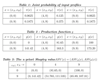
Example 4. (Firm and suppliers) An economy consists of a firm and two suppliers A and B who
respectively supply inputsxA andxB to the firm, with xA∈ {0,4,9} andxB∈ {0,9}. The firm’s technology
is represented by the constant elasticity of substitution production functiong(xA, xB) = 100(13x1/2A +23x 1/2 B )1/2.
SupplierAprovides 0 units of commodityxA with probability 0.25, 4 units of this commodity with probability
0.5, and 9 units with probability 0.25. Supplier B provides 0 units of commodity xB with probability 0.25,
and 9 units with probability 0.75. We also assume that the price of each output produced is equal to 1, so
that for an input profilex= (xA, xB),g(x)also represents the revenue of the output generated byx. Table 1
shows the probability of realizing each profile of inputs. Table 2 presents the production function of the firm,
[image:10.595.155.492.324.597.2]and Table 3 presents the a prioriShapley value of the two suppliers for each input profile.
Table 1: Joint probability of input profiles
x= (xA, xB) π(x) x= (xA, xB) π(x) x= (xA, xB) π(x)
[image:10.595.162.487.338.411.2](0,0) 0.0625 (4,0) 0.125 (9,0) 0.0625 (0,9) 0.1875 (4,9) 0.375 (9,9) 0.1875
Table 2 : Production functiong
x= (xA, xB) g(x) x= (xA, xB) g(x) x= (xA, xB) g(x)
[image:10.595.165.482.431.555.2](0,0) 0 (4,0) 81.65 (9,0) 100 (0,9) 141.42 (4,9) 163.3 (9,9) 173.20
Table 3: The a priori Shapley valueASV(x) = (ASVA(x), ASVB(x))
xB↓ xA→ 0 4 9
0 (0,0) (81.65,0) (100,0) 9 (0,141.42) (51.765,111.535) (65.89,107.31)
Using the information in Tables 1–3, we derive the a prioriShapley value for the production environment
P = (N,(TA, TB), g, π) (N ={A, B},TA={0,4,9},TB={0,9}, andT =TA×TB) as follows:
ASVA(P) =
X
x∈T
π(x)ASVA(x) = 48.2225and ASVB(P) =
X
x∈T
π(x)ASVB(x) = 88.4625.
Each supplier is therefore expected to have a different effect on the output of the firm. This is for three
reasons. The first is that the suppliers are not interchangeable in the production process, as illustrated by
Table 2. The second reason is that they do not supply inputs with the same probability, and the third is that
[image:10.595.170.480.525.590.2]The next example shows how the a priori Shapley value can be applied to a financial system of banks (see, e.g., Allen and Gale (2000), Battiston et al.(2012), Lin (2016)) in order to measure the contribution of each bank to systemic risk.3
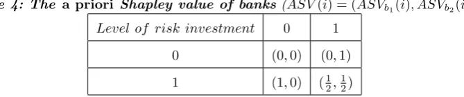
Example 5. (Measuring financial risk) Assume a financial market in which banks are connected and
investments are highly correlated. For simplicity, assume that there are only two banksb1 andb2 which have
up to two choices of risk investments. Each bank may decide to avoid any risk investment – which corresponds
to choice 0 – or to invest some part of its assets in the risky activities, corresponding to choice 1. A global risk
functionhmaps a vector of investment choices to a risk measure. The probability distributionπover the set
of choicesIA={0,1}=IB is given as follows:πb1(0) = 0.6,πb1(1) = 0.4,πb2(0) = 0.25, and πb2(1) = 0.75.
The risk measure functionhis given by:
h(i) =
1 if i6= (0,0) 0 if i= (0,0)
(4)
[image:11.595.161.496.381.451.2]The a prioriShapley value of each bank is given in Table 4 below:
Table 4: The a priori Shapley value of banks(ASV(i) = (ASVb1(i), ASVb2(i)))
Level of risk investment 0 1 0 (0,0) (0,1) 1 (1,0) (1
2, 1 2)
The a prioriShapley valueASV(x)measures the contribution of each bank to systemic risk at investment profile x. The expected contribution of each bank to systemic risk in the uncertain environment defined by
P = (N ={b1, b2},(IA, IB), h, π)is given hereunder:
ASVb1(P) = 0.25and ASVb2(P) = 0.6.
These values illustrate the fact that banks that are more likely to invest in risky activities contribute more
to the failure of the overall system.
4
The Bayesian Shapley Value
This section is devoted to the problem of valuing inputs a posteriori; that is, after the realization of the output. LetP = (N,(Ti)i∈N, f, π) be an uncertain production environment. Assume that an output levelY
is realized. Given the prior probability distribution πi of each input variablei, we can derive the posterior
probability distributions using Bayesian updating. We then apply these posterior probability distributions to obtain what we call the Bayesian Shapley value, and we provide an axiomatic characterization of this value.
3
To illustrate, imagine a firm in which the manager observes the level of output Y, but cannot observe the inputs (or ability) of workers. The realized output has to be shared among the workers. What share of this output should the manager give each worker? In answering this question, we assume that the manager is Bayesian and that she has prior beliefs about the distribution of inputs (that is, she knowsπ).
Consider a simple case where there are exactly three input profilesx,y andz such that f(x) =f(y) =
f(z) =Y. The prior probabilities of these profiles areπ(x),π(y) andπ(z), respectively. The prior probability of the realization ofY is therefore:
P(Y) =π(x)P(Y|x) +π(y)P(Y|y) +π(z)P(Y|z).
SinceP(Y|x) =P(Y|y) =P(Y|z) = 1, it follows that P(Y) =π(x) +π(y) +π(z). We note that this sum is not necessarily equal to 1. Using Bayes’ theorem, the posterior probability that we are looking for is obtained by dividing the prior probability byP(Y). For eachh∈ {x, y, z}, we then have:
P(h|Y) = P(Y ∩h)
P(Y) = P(h)×P(Y|h)
P(Y) = π(h)
π(x) +π(y) +π(z), sinceP(h) =π(h) andP(Y|h) = 1.
Knowing the posterior probability distribution {P(h|Y)} over the set{x, y, z}, the average value (AV) of inputiis:
AVi(Y) = ASVi(x)P(x|Y) +ASVi(y)P(y|Y) +ASVi(x)P(z|Y)
= π(x)ASVi(x) +π(y)ASVi(y) +π(z)ASVi(z)
π(x) +π(y) +π(z) .
We will call this valuation scheme the Bayesian Shapley value. Below, we generalize this scheme to any uncertain production environment. Let P = (N,(Ti)i∈N, f, π) be an uncertain production environment.
Denote by Rf = {Y ∈R:∃x∈T, f(x) =Y} the set of realizable outputs. For any Y ∈ Rf, define by
Yf ={x∈T :f(x) =Y}the set of input profiles that produceY. We have the following definition.
Definition 3. The Bayesian Shapley value is the function BSA defined, for any uncertain production environmentP = (N,(Ti)i∈N, f, π) and any realizable outputY ∈ Rf, by:
BSAi(Y) =
P
x∈Yf
π(x)ASVi(x)
P
x∈Yf
π(x) , i∈N. (5)
We now want to present an axiomatic characterization of this value. A few preliminary notions will be needed. For any uncertain production environmentP= (N,(Ti)i∈N, f, π) and any realizable outputY ∈ Rf,
is the posterior probability distribution over input profiles and is defined as follows:
P(h|Y)=
π(h)
P
x∈Yf
π(x) if h∈Yf
0 if h /∈Yf
(6)
We also define the notion of symmetrya posteriori.
Definition 4. LetP = (N,(Ti)i∈N, f, π) be an uncertain production environment andY ∈ Rf a realizable
output. Two input factorsi andj are said to be symmetric a posteriori if for any input profilex∈Yf such
thatxi= 0 orxj= 0, f(x) =f(τij(x)).
We now present the axioms.
Axiom 4. (Symmetry a posteriori)
A valuation procedure φis symmetric a posteriori if for any production environmentP = (N,(Ti)i∈N, f, π),
any realizable output Y ∈ Rf, and any input factors i and j that are symmetric a posteriori, φi(PY) =
φj(PY).
Axiom 5. (Efficiency a posteriori)
A valuation procedureφis efficient a posteriori if for any production environmentP = (N,(Ti)i∈N, f, π)and
any realizable outputY ∈ Rf, P i∈N
φi(PY) =Y.
Axiom 6. (Marginality a posteriori)
A valuation procedureφsatisfies the axiom of marginality a posteriori if for any production environmentP = (N,(Ti)i∈N, f, π), any realizable output Y ∈ Rf, any production environment P′ = (N,(Ti)i∈N, g, P(.|Y)),
any inputi∈N, and any input profilesx∈Yf anda∈T such that a⊳i0x:
[g(a+xiei)−g(a)≥f(a+xiei)−f(a)]⇒[φi(P′)≥φi(PY)].
The axiom of symmetry a posteriori states that inputs that are interchangeablea posteriori should be identically valued. The axiom of efficiency a posteriori states that any realized output Y of an uncertain production environment should be entirely shared among the different inputs. The axiom of marginality a posteriori states that, if there is a change in the technology that increases the marginal productivity of an input in the posterior production environment of an uncertain production environment, then the valuation procedure should give a greater value to that input under the new technology.
The theorem below states that the Bayesian Shapley value is the only valuation scheme that satisfies all three axioms above.
Theorem 2. The Bayesian Shapley value is the only valuation procedure that satisfies simultaneously the
axioms of symmetry a posteriori, efficiency a posteriori, and marginality a posteriori.
Theorem 3. For any uncertain production environment P = (N,(Ti)i∈N, f, π) and any input i ∈ N, we
have:
Ui(f) =
X
Y∈Rf
P(Y)BSAi(Y) =
X Y∈Rf X
x∈Yf
π(x)ASVi(x)
=ASVi(f).
The following example applies the notion of the Bayesian Shapley value to an epidemiological context.
Example 6. (Assessing the risk factors of a disease) A disease (e.g., type 2 diabetes) is caused by a
set of four leading behavioral and dietary risk factors which are: low fruit and vegetable intake (risk factor
1), smoking (risk factor 2), high body mass index (risk factor 3), and high blood pressure (risk factor 4).
Let Ti = {0,1} be the set of values that each risk factor i can take, and f the production function of the
disease. The production function, given in Table 5 below, determines the probability (in percentage terms)
that an individual with a given profile will have the disease. For example, if an individual has the risk profile
(1,0,0,0) – that is, the individual has low fruit and vegetable intake and no other risks – his probability of getting the disease is 5%. Also, an individual who has the risk profile (1,1,0,1)– that is, the individual who has low fruit and vegetable intake, smokes, and has high blood pressure – has a 30% chance of getting the
disease.
For each risk profiler= (r1, r2, r3, r4)∈T = 4
Q
i=1
Ti, we compute the contribution of each risk factori to
the probability of getting the disease. The results are presented in Table 5. Remark that these contributions
[image:14.595.158.490.460.647.2]sum to f(r) for each risk profiler.
Table 5: Values of f(r) andASV(r)
r f(r) ASV(r) r f(r) ASV(r) (0,0,0,0) 0 (0,0,0,0) (1,0,0,0) 5 (5,0,0,0) (0,0,0,1) 20 (0,0,0,20) (0,1,0,1) 25 (0,5,0,20) (0,0,1,0) 10 (0,0,10,0) (0,0,1,1) 30 (0,0,10,20) (0,1,0,0) 5 (0,5,0,0) (0,1,1,0) 13 (0,4,9,0) (1,0,0,1) 25 (5,0,0,20) (1,0,1,1) 50 (606,0,906,1506 ) (1,1,0,0) 7 (3.5,3.5,0,0) (1,1,0,1) 30 (276,276,0,1266 ) (1,0,1,0) 15 (5,0,10,0) (1,1,1,0) 20 (31
6, 25
6, 64
6,0)
(0,1,1,1) 50 (0,58 6,
88 6,
154
6 ) (1,1,1,1) 70 ( 238 24, 230 24, 482 24, 730 24)
We now assume that each risk factor is uniformly distributed overTi. That is,πi(0) =πi(1) = 0.5for each
risk factor i∈N ={1,2,3,4}. The prior Shapley value of each risk factoriis ASVi(P) = 161 P r∈R
ASVi(r).
We therefore have:
ASV1(P) = 3.005, ASV2(P) = 2.838, ASV3(P) = 6.213, and ASV4(P) = 11.38.
Assume that the social planner observes that the prevalence of the disease is 50% in a subgroup of the
the disease in that subgroup. The goal is to identify those risk factors in which society can invest in order to
reduce the prevalence of the disease.
Based on the prior information concerning the outcome of each risk profile, there exist only two risk
profiles that lead to a prevalence of 50%:r= (0,1,1,1) andr′= (1,0,1,1). The Bayesian Shapley value for
each risk factoriis therefore given by:
BSAi=
π(r)ASVi(r) +π(r′)ASVi(r′)
π(r) +π(r′) =
1
2(ASVi(r) +ASVi(r
′)), f or i∈ {1,2,3,4}.
Using the information above, we have :BSA1= 5, BSA2= 4.83, BSA3= 14.83, and BSA4= 25.34. High
blood pressure is therefore the most significant contributor to the disease, as it accounts for more than half
of its prevalence in that population subgroup. It is followed by high BMI, low fruit and vegetable intake, and
smoking.
5
Rationalizable Probability Distributions
So far, we have considered a production environmentP = (N,(Ti)i∈N, f, π) where the supply of input factors
is uncertain, with the uncertainty captured by an exogenous profile of the probability distributionsπ. This model can be justified in real-life situations where exogenous shocks affect the supply of inputs, such as when the performance of a worker depends on weather conditions. But there also exist situations in which inputs, viewed as rational players, may choose probability distributions that maximize their payoffs. In this section we ask whether certain probability distributions can be rationalized.
In order to answer this question, we consider a modified production environment (N,(Ti)i∈N, f) without
uncertainty, and we associate to this environment a finite strategic form gameG= (N, T,(ui)i∈N) where the
payoff functionsui(x) are given by the Shapley wage functions ASVi(x) under the technologyf.4
Here, each playerichooses from his strategy set Ti the amount of labor he wishes to supply to the firm.
A profilex= (x1, x2, ..., xn)∈T (recall thatT = n
Q
i=1
Ti) of effort levels is a profile of pure strategies. Instead
of choosing a single action, players can also randomize over the set of available actions according to some probability distribution similar toπunder the uncertain production environmentP. Such a behavior would define a mixed strategy profile.
For each player i, we denote by Si = Si(Ti) the set of all probability distributions over Ti. The set
S =S1×S2×...×Sn is therefore the set of mixed strategy profiles. Let si ∈Si be a mixed strategy of
a player i. By si(xi), we denote the probability with which action xi is played under the mixed strategy
si∈Si. The subset of pure strategies that are assigned positive probability by the mixed strategysiis called
the support ofsi. A pure strategy is a special case of a mixed strategy in which the support is a singleton.
ui(x) =ASVi(x) for everyx∈T.
Let (N,(Ti)i∈N, f) be an environment and s= (s1, s2, ..., sn) a mixed strategy profile of the associated
gameG. Then the tuplePs= (N,(T
i)i∈N, f, s) is an uncertain production environment. The expected payoff
of each player inPsis also his expected payoff in the gameG whensis played. This expected payoff is:
ui(s) =ASVi(Ps) =
X
x∈T
s(x)
X
a⊳i
0x
(|a|)!(|x| − |a| −1)!
(|x|)! [f(a+xiei)−f(a)]
; with s(x) = Y
j∈N
sj(xj).
In the case of pure strategies, meaning that a profilexoccurs with certainty, the utility of playeriatxis:
ui(x) =ASVi(x) =
X
a⊳i
0x
(|a|)!(|x| − |a| −1)!
(|x|)! [f(a+xiei)−f(a)].
We recall the following definitions:
Definition 6. LetG be the game associated to a production environment (N,(Ti)i∈N, f). A playeri’s best
response to a strategy profile s−i is a mixed strategy s∗i ∈ Si such that ui(s−i, s∗i) ≥ ui(s−i, si) for all
strategiessi ∈Si.
Definition 7. A strategy profiles∗= (s∗
1, s∗2, ..., s∗n) is a Nash Equilibrium of a game (N, T,(ui)i∈N) if, for
all playeri,s∗
i is a best response tos∗−i.
Equivalently, s∗= (s∗
1, s∗2, ..., s∗n) is a Nash Equilibrium of a game (N, T,(ui)i∈N) if and only if for every
playeri:
ui(s∗) = max all s′
is
ui(s∗−i, si) (7)
We have the following result, which states that there always exists a rationalizable profile of probability distributions in any production environment.
Theorem 4. There always exists a rationalizable profile of probability distributions in any environment
(N,(Ti)i∈N, f). Equivalently, the game(N, T,(ui)i∈N)associated to any production environment(N,(Ti)i∈N, f)
admits a mixed strategy Nash equilibrium.
Since the game associated with a production environment is finite, the proof of this result simply follows from the proof of the existence of a mixed strategy Nash equilibrium in finite games (Nash (1951)).
We now present a natural property of the production function that ensures the existence of a pure strategy Nash equilibrium in the associated finite game.
Definition 8. Let (N,(Ti)i∈N, f) be a production environment. The functionf satisfies the positive
inter-action property (PIP) if for allx, y∈T, f(x)≤f(y) if and only ifxy, where xy⇔xi≤yi ∀i∈N.
Theorem 5. Let (N,(Ti)i∈N, f) be an environment such that the function f satisfies PIP. Its associated
game(N, T,(ui)i∈N) admits a pure strategy Nash equilibrium.
A key implication of this result is that the non-cooperative game associated with any monotonic von Neumann-Morgernstern transferable-utility game (i.e.,Ti={0,1}) admits a pure strategy Nash equilibrium
under the Shapley wage function. That equilibrium is such that each player chooses action 1. Interestingly, this finding provides a condition under which the assumption of the grand coalition can be justified or rationalized in the calculation of the Shapley value in the classical work of Shapley (1953). As shown in the examples below, relaxing this condition may lead to other equilibria emerging, which illustrates the existence of a more general set of rationalizable profiles of probability distributions in a production environment.
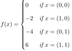
Example 7. Consider the production environment(N,(Ti)i∈N, f), whereN ={1,2},T1={0,1}=T2, and
the production functionf is defined as follows:
f(x) =
0 if x= (0,0)
−2 if x= (1,0)
−4 if x= (0,1) 6 if x= (1,1)
.
[image:17.595.260.380.333.418.2]The Shapley payoffs derived from the associated strategic game(N, T,(u1, u2))are displayed in Table 6 below:
Table 6: Payoffs(u1(x), u2(x))
Player 2
strategies 0 (β) 1 (1−β)
Player 1 0 (α) (0,0) (0,−4) 1 (1−α) (−2,0) (4,2)
The profile π = (π1, π2) such that π1(0) = α, π1(1) = 1−α, π2(0) = β, and π1(1) = 1−β, with
0≤α, β≤1, represents a profile of probability distributions over the set of pure strategies. We find that the strategic form game has two pure strategy Nash equilibria which are (0,0) and(1,1). The game also has a mixed strategy Nash equilibrium in which player 1 chooses the effort level0with probability 13, whereas player 2 chooses the effort level 0 with probability 2
3. There are therefore three rationalizable profiles of probability
distributions in this game:((1,0),(1,0)),((0,1),(0,1)), and((1 3,
2 3),(
2 3,
1 3)).
Example 8. Consider a production environment with three workers and two effort levels 0 and 1. The
production function is the following:
f(x) =
1 if |x| ∈ {2,3}
0 otherwise .
Table 7: Effort profile (x)and Shapley wage profile((u1(x), u2(x), u3(x))).
x (u1(x), u2(x), u3(x)) x (u1(x), u2(x), u3(x))
(0,0,0) (0,0,0) (0,1,1) (0,1 2,
1 2)
(0,0,1) (0,0,0) (1,0,1) (12,0,12) (0,1,0) (0,0,0) (1,1,0) (1
2, 1 2,0)
(1,0,0) (0,0,0) (1,1,1) (1 3,
1 3,
1 3)
The pure strategy Nash equilibria are (0,0,0) and (1,1,1). We want to determine whether there exist other equilibria. Let Si be the set of player i’s mixed strategies. Then S1 ={(α,1−α) :α∈[0,1]}, S2 =
{(β,1−β) :β ∈[0,1]}, and S3 = {(γ,1−γ) :γ∈[0,1]}. Consider a mixed strategy profile s = ((α,1−
α),(β,1−β),(γ,1−γ)). We derive the expected payoff at the profile sas follows:
E1(s) = (1−α)
1
3(1−γ)( 1
2β+ 1) + 1
2γ(1−β)
,
E2(s) = (1−β)
1
3(1−γ)( 1
2α+ 1) + 1
2γ(1−α)
,
E3(s) = (1−γ)
1
3(1−β)( 1
2α+ 1) + 1
2β(1−α)
.
Playerirandomizes between strategies 0 and 1 if and only if he is indifferent between them; that is,ui(s|α=
1) =ui(s|α= 1). Thus, we have the following:
E1(s|α= 1) =u1(s|α= 0) if and only if γ= β+ 2
4β−1; (8)
E2(s|β= 1) =u2(s|β = 0)if and only if α=
γ+ 2
4γ−1; (9)
E3(s|γ= 1) =u3(s|γ= 0)if and only if β =
α+ 2
4α−1. (10)
Equations (8), (9) and (10) lead to the system:(S)
γ=4ββ+2−1 (a) α=4γγ+2−1 (b) β= α+2
4α−1 (c).
Substituting expression γ from equation(a)into equation (b) leads to α=β (d). Rewriting equation (c)
under condition (d) gives equation 2α2−α−1 = 0 (e). The latter equation has two roots: α = −1 2 and
α= 1. Since αis positive, we can conclude that there are only two rationalizable probability distributions in this game that correspond to the pure strategy Nash equilibria (0,0,0)and(1,1,1).
6
An Application to Contagion in a Networked Economy
[image:18.595.216.438.300.389.2]Consider an economy M involving agents who freely form and sever bilateral links according to their preferences. Assume that rational behavior is captured by a certain equilibrium notion (e.g., pairwise stability, stochastic stability, etc.). Such an economy may have multiple equilibria. Denote by E(M) the set of its equilibria. Our goal is twofold. First, we would like to evaluate the expected contribution of each agent (or node) to the spread of a random infection that might hit the economy. Second, given an observed contagion level, we would like to determine the contribution of each agent to that level.
To illustrate these notions, consider a fidelity economyMinvolving two menm1andm2and two women
w1 and w2. Man m1 desires one female partner; man m2 desires two female partners; and each woman
desires only one male partner.5 A network is a collection of links between men and women. This economy
can be represented by an uncertain production environment (N,(Ti)i∈N,f , πe ), whereN ={m1, m2, w1, w2};
Tm1 ={∅,{w1},{w2}};Tm2 ={∅,{w1},{w2},{w1, w2}};Tw1 ={∅,{m1},{m2}}; Tw2 ={∅,{m1},{m2}}, fe
is a contagion function (see below), andπis a probability distribution over the set of input profiles. For simplicity, denote{w1} by 1,{w2}by 2, {m1}by 3, {m2}by 4, {w1, w2}by 5, and the empty set∅
by 0. The input profilex= (1,5,4,4), for instance, means thatm1 desires to match withw1,m2 desires to
match withw1 andw2, w1 desires to match withm2, andw2 desires to match withm2. A match between
two individuals occurs if it is desired by both. The input profilex= (1,5,4,4) therefore leads to the network
g2in Figure 1 below. If at an input profilex,xi= 0 for an individuali, it means thatiwants no partner. It
follows from this interpretation that each input profilex∈T = Q
i∈N
Ti is a network.
[image:19.595.180.467.565.656.2]Assume that rationality is captured by the notion of pairwise stability as defined in Pongou and Serrano (2013, 2016). A networkgis pairwise stable if: (i) no individual has an incentive to sever an existing link in which he is involved; and (ii) no pair of a man and a woman has an incentive to form a new link while at the same time severing some of the existing links in which they are involved. There are 8 possible networks in this economy, but only 3 of them are pairwise stable. These equilibrium networks are represented by the graphs below:
Figure 1: pairwise stable networks
The contagion function is the contagion potential of a network (Pongou (2010)). To define this function, letgbe ann-person network that haskcomponents, where a component is a maximal set of agents who are
5
directly or indirectly connected ing; and nj the number of individuals in the jth component (1 ≤j ≤k).
Pongou (2010) (see also Pongou and Serrano (2013, 2016)) shows that if a random individual is infected with a virus (e.g., HIV), and if that individual infects his/her partners who also infect their other partners and so on, the fraction of infected people is given by the contagion potential ofg, which is:
P(g) = 1
n2 k
X
j=1
n2j.
We can also derive the part of contagion for which agents are collectively responsible ing. It is:
e
f(g) =P(g)− 1
n.
This expression is justified because each individual in g is exogenously infected with probability 1 n, and
agents are not responsible for exogenous infections.
Following this formula, we calculate the contagion potential of each equilibrium network:
P(g1) =
1 42(2
2+ 22) = 0.5,P(g
2) = 0.625, andP(g3) = 0.5.
Our goal is being able to determine the responsibility of each agent for the level fe(g) of transmitted contagion in a networkg. LetS be a set of agents. We denote byg(S) the restriction of the networkgtoS. This restriction is obtained by severing all the links involving agents in N\S. Also, leti be an individual. We denote byg(S) +ithe networkg(S∪ {i}) obtained fromg(S) by connecting ito all the agents inS to whomiis connected in the networkg. Thea priori Shapley value of each individualiin the networkg is:
Pi(g) =
X
S⊆N,i /∈S
s!(n−s−1)!
[image:20.595.179.466.557.636.2]n! [P(g(S) +i)− P(g(S))], s=|S|. (11) Thea priori Shapley value for each agent in each equilibrium network is given by Table 8.
Table 8: Individual contagion potential in equilibrium networks
Stable networks(g) Pm1(g) Pm2(g) Pw1(g) Pw2(g)
g1 161 161 161 161
g2 0 488 485 485
g3 161
1 16
1 16
1 16
Remark that in each network g, the contagion potentials (Shapley values) of agents sum up tofe(g), so that the contagion potential of each agent measures his/her responsibility for the transmitted contagion.
Only equilibrium networks are likely to form. Therefore, the a priori Shapley value of an agent i to contagion in the economyMis:
Pi(M) =
X
g∈E(M)
π(g)Pi(g). (12)
pairwise meetings as follows. Assume that men and women meet randomly and decide whether to form a link or not. For instance, consider a possible order of meetingr= ({m1, w1},{m1, w2},{m2, w1},{m2, w2}),
interpreted as follows: agents m1 and w1 meet first; then agents m1 and w2 meet; then agentsm2 and w1
meet; finally agentsm2andw2meet. At each meeting, the meeting agents form a link if they mutually desire
each other and have not reached yet their optimal number of partners. The order meetingr above will lead to the networkg1. There are 24 meeting orders in total. If we assume each order to be equally likely, then we
find the following probability of formation for each network:π(g1) = 0.375,π(g2) = 0.25, andπ(g3) = 0.375.
Using this probability distribution, we compute the contagion potential of each individual in the mating economyMas follows:
ASVm1(M) = 0.046875,ASVm2(M) = 0.0885, andASVw1(M) =ASVw2(M) = 0.0729.
Clearly, we see thatm2has the highest contagion potential, which is justified by the fact that his demand
for partners is the highest.
Now, assume that the prevalence of the infection in the population is 25%. We are interested in determin-ing the responsibility of each agent for the contagion. There exist only two networks that lead to a contagion prevalence of 25%, namelyg1 andg3(recall thatfe(g1) =fe(g3) =P(g1)−0.25 =P(g3)−0.25 = 0.25). The
Bayesian Shapley value is therefore:
BSAi=
π(g1)Pi(g1) +π(g3)Pi(g3)
π(g1) +π(g3)
, f or i∈ {m1, m2, w1, w2}.
Using the information above, we have :BSAm1 =BSAm2 =BSAw1 =BSAw2 = 0.0625.
Importantly, whereas the a priori Shapley value depends on the structure of economy, the Bayesian Shapley value depends on the structure of the equilibrium network that possibly realizes. As shown by the example above, these values can be very different.
7
Conclusion
References
Aguiar, V. H., Pongou, R., and Tondji, J. B. (2016). Measuring and decomposing the distance to the Shapley wage function with limited data. Mimeo.
Allen, F., and Gale, D. (2000). Financial contagion.Journal of political economy, 108(1), 1-33.
Battiston, S., Gatti, D. D., Gallegati, M., Greenwald, B., and Stiglitz, J. E. (2012). Liaisons dangereuses: Increasing connectivity, risk sharing, and systemic risk.Journal of Economic Dynamics and Control, 36(8), 1121-1141.
Freixas, J. (2005). The Shapley-Shubik power index for games with several levels of approval in the input and output.Decision Support Systems, 39, 185-195.
Gale, D., and Shapley, L., (1962). College admissions and the stability of marriage.American Mathematical Monthly 69, 9-15.
Hsiao, Chih-Ru, and Raghavan T.E.S. (1993). Shapley value for multichoice cooperative games, I. Games and Economics Behavior, 5, 240-256.
Lin, J. (2016). Using weighted Shapley values to measure the systemic risk of interconnected banks. Pacific Economic Review.
Nash, F. J. (1951). Non-cooperative games.The Annals of Mathematics, 54(2), 286-295.
Pongou, R. (2010). The economics of fidelity in network formation. PhD Dissertation, Brown University. Pongou, R., and Serrano, R. (2013). Fidelity networks and long-run trends in HIV/AIDS gender gaps.The
American Economic Review, 103(3), 298-302.
Pongou, R., and Serrano, R. (2016). Volume of trade and dynamic network formation in two-sided economies.
Journal of Mathematical Economics, 63, 147-163.
Pongou, R., and Tondji, J-B. (2016).Non-cooperative games with Shapley payoffs. Working paper. Roth, A. (1988). The Shapley value: essays in honor of Lloyd S. Shapley, Cambridge University Press.
Serrano, R. (2013). Lloyd Shapley’s matching and game theory. Scandinavian Journal of Economics, 115, 599-618.
Shapley, L. (1953). A Value for n-person games.In Contributions to the Theory of Games, 2 , 307-317.
Shapley, L., and Shubik, M. (1967). Ownership and the production function. The Quarterly Journal of Economics, 88-111.
8
Appendix
In order to prove Theorem 1, we need to establish some preliminary results. Define the following production functionfxfor each x∈T by:
fx(y) =
1 if xEy
0 if x5y
(13)
The following lemma, proved in Aguiar et al.(2016), shows that every production function is a linear combi-nation of these basic functions.
Lemma 1. Any production function is a linear combination of the production functionsfx:
f = X
x∈T; x6=0
cx(f)fx, wherecx(f) =
X
x′Ex
(−1)|x|−|x′|f(x′). (14)
In order to prove Theorem 1, we also need to show that thea prioriShapley value satisfies the probabilistic additivity property defined below.
Definition 9. A valuation procedure φ is probabilistically additive if for any uncertain production environmentP = (N,(Ti)i∈N, f, π) andP′ = (N,(Ti)i∈N, g, π),φ(f +g) =φ(f) +φ(g).
We now state the following result.
Lemma 2. The a priori Shapley valueASV is probabilistically additive.
Proof. LetP = (N,(Ti)i∈N, f, π) and P′ = (N,(Ti)i∈N, g, π) be two production environments. Consider an
inputi∈N; then we have:
ASVi(f +g) =
X
x∈T
π(x)nASVif+g(x)o,
where:
ASVif+g(x) = X
a⊳i
0x
(|a|)!(|x| − |a| −1)!
(|x|)! {(f+g)[a+xiei]−(f+g)[a]}
= X
a⊳i
0x
(|a|)!(|x| − |a| −1)!
(|x|)! {mc(, i, f, a, x)}
+ X
a⊳i
0x
(|a|)!(|x| − |a| −1)!
(|x|)! {mc(i, g, a, x)} = ASVif(x) +ASVig(x).
We can conclude thatASVi(f+g) = P x∈T
π(x)ASVif(x) +
P
x∈T
π(x)ASVig(x) =ASVi(f) +ASVi(g), andASV
Now, we are ready to prove Theorem 1.
Proof of Theorem 1
A. Sufficiency
In this part of the proof, we show that thea priori Shapley valueASV satisfies the axioms of probabilistic symmetry, marginality, and probabilistic efficiency.
LetP = (N,(Ti)i∈N, f, π) be an uncertain production environment.
1. Probabilistic symmetry: Letiandj be two probabilistically symmetric inputs. Then:
ASVi(f) =
X
x∈T, xi=xj
π(x)ASVi(x) +
X
x∈T, xi>xj
π(x)ASVi(x) +
X
x∈T, xi<xj
π(x)ASVi(x).
Thea priori Shapley value of input iat a given input profilexis given by:
ASVi(x) =
X
a⊳i
0x
ϕ(a, x)[f(a+xiei)−f(a)]
= X
a⊳i
0x and aj=0
ϕ(a, x)[f(a+xiei)−f(a)] +
X
a⊳i
0x and aj6=0
ϕ(a, x)[f(a+xiei)−f(a)]
= X
b⊳j0x and bi=0
ϕ(b, x)[f(a+xiej)−f(a)]
+ X
b⊳j0x and bi6=0, b=a−xjej+xjei
ϕ(b, x)[f(b+xiej)−f(b)].
Note that for any x, y ∈ T such that: (xi = a and xj = b), (yj = a and yi = b), and yk = xk for
any k6=i, j, we haveASVi(x) =ASVj(y). Moreover, given that πi =πj, we haveπ(x) =π(y). Since
ASVi(x) =ASVj(x) for allxsuch thatxi=xj, we can conclude that:
ASVi(P) =
X
x∈T, xi=xj
π(x)ASVj(x) +
X
x∈T, xj>xi
π(x)ASVj(x) +
X
x∈T, xj<xi
π(x)ASVj(x)
= ASVj(P).
2. Marginality: consider a production environment P′ = (N,(T
i)i∈N, g, π) such that mc(i, f, a, x) ≥
mc(i, g, a, x) for alli∈N,x, a∈T anda⊳i0x. By the definition of thea priori Shapley value, we have
ASVif(x)≥ASV g
i (x). Hence,
P
x∈T
π(x)ASVif(x)≥
P
x∈T
π(x)ASVig(x), that isASVi(f)≥ASVi(g), or
equivalently,ASVi(P)≥ASVi(P′).
3. Probabilistic efficiency: for the production environmentP, we have:
X
i∈N
ASVi(P) =
X
i∈N
X
x∈T
π(x)ASVi(x)
= X
x∈T
π(x)
( X
i∈N
ASVi(x)
)
= X
x∈T
π(x)f(x), since X
i∈N
B. Necessity
In this part of the proof, we prove the uniqueness of thea priori Shapley value. Consider another allocation procedure φ which satisfies the axioms of probabilistic efficiency, marginality and probabilistic symmetry. We would like to show that, for any production environment P = (N,(Ti)i∈N, f, π), φi(f) =ASVi(f) for
each inputi∈N.
1. Consider a production functionf which is identically zero on all input profiles. Then
mc(i, f, a, x) = 0f or all x, a∈T such that a⊳x; .
Given thatφsatisfies the probabilistic symmetry axiom, we have φi(f) =φj(f) forj6=i, and by the
probabilistic efficiency axiom, we have:
X
i∈N
φi(f) =
X
x∈T
π(x)f(x) = 0.
Hence, φi(f) = 0 for each input i ∈ N. We can show in the same manner that for any production
function f onT, an input profile x∈T, and anyi∈N:
if mc(i, f, a, x) = 0f or all x, a∈T such that a⊳x, then φi(f) = 0. (15)
Iff ≡0, we also haveASVi(f) = P x∈T
π(x)ASVi(x) = 0, sinceASVi(x) = 0 for allx.
2. Letf be a production function, then by using Lemma 1, we can write:
f(y) = X
x∈T, x6=0
cx(f)fx(y). (16)
By the definition offx, the latter expression (equation (16)) can be rewritten as:
f(y) = X
x∈T, x6=0, xEy
cx(f)fx(y) =
X
x∈T, x6=0, xEy
cx(f).
It follows that for i∈N:
φi(f) =φi
X
x∈T, x6=0, xEy
cx(f)fx(y)
=φi
X
x∈T, x6=0, xEy
cx(f)
.
Define the indexI of the production functionf to be the minimum number of non-zero terms in some expression forf of the form established in Lemma 1. The theorem is proved by induction onI.
a) IfI= 0, thenf ≡0. By the probabilistic efficiency requirement, we have:
X
i∈N
φi(f) =
X
x∈T
π(x)f(x) = 0.
Using the probabilistic symmetry axiom, we have |N|φi(f) = 0, which implies that φi(f) = 0.
b) If I = 1, then f = cx(f)fx for some x ∈ T. Thus, φi(f) = φi(cx(f)fx). Consider Xx =
{l∈N:xl>0}and leti /∈Xx. Fora, x∈T such thata⊳i0x, we havef(a+xiei)−f(a) = 0, i.e
mc(i, f, a, x) = 0. It follows from equation (15) and from the fact thatφi satisfies the marginality
axiom thatφi(f) = 0. Moreover,ASVi(x) = 0 for allx, leading toASVi(f) = 0. Leti, j∈N such
that i, j∈Xx. Let us show that iandj are probabilistically symmetric.
• Consider y ∈ T such that yi =yj = 0. We have f(y) = cx(f) if xEy. Since i, j ∈ Xx, it
means thatxi>0 andxj>0. Then,x5y andf(y) =f(τij(y)) = 0.
• Consider y∈T such that (yi = 0 andyj 6= 0) or (yj = 0 and yi 6=yj). For the same reason
stated above,f(y) =f(τij(y)) = 0.
We can conclude that inputsi andj are probabilistically symmetric. Using the axioms of proba-bilistic symmetry and probaproba-bilistic efficiency, we have:
|x|φi(f) =
X
xEy, y∈T
π(y)cx(f),
so that,
φi(f) =
P
xEy, y∈T
π(y)cx(f)
|x| =ASVi(f).
c) Assume now thatφis the value ASV whenever the index of f is at mostI and letf have index
I+ 1, with:
f =
I+1
X
k=1
cxk(f)fxk, all cxk 6= 0, and xk∈T.
Fork∈ {1,2, ..., I+ 1}, consider:
Xk =
l∈N :xkl >0 , X= I+1\
k=1
Xk, and assume i /∈X.
Define the following production function:
g= X
k:i∈Xk
cxk(f)fxk.
The index ofgis at mostI. Letx, a∈Tsuch thata⊳i0x. Thenf(a+xiei)−f(a) =g(a+xiei)−g(a).
Hence, using the marginality axiom, φi(f) =φi(g). By induction, we have:
φi(f) =
X
k:i∈Xk
P
y∈T, xkEy
π(y)cxk(f)
|xk|
,
which is the value ofASVi(f) by using the aforementioned properties.
It remains to show that φi(f) = ASVi(f) when i ∈ X. By the probabilistic symmetry axiom,
φi(f) is a constantǫ for all members ofX; likewise the valueASVi(f) is some constantǫ′ for all
members ofX. Since both allocations sum to P
x∈T
π(x)f(x) and are equal for all i∈X, it follows
Proof of Theorem 2: The proof follows the same reasoning as that of Theorem 1.
Proof of Theorem 3: Consider a production environmentP = (N,(Ti)i∈N, f, π). In order to establish
the proof, it suffices to show that the value U satisfies the axioms of marginality, probabilistic symmetry, and probabilistic efficiency. We recall that:
Ui(f) =
X
Y∈Rf
P(Y)BSAi(Y),
where Rf ={Y ∈R:∃x∈T, f(x) =Y} is the set of realizable outputs andYf ={x∈T :f(x) =Y} for
Y ∈ Rf.
1. First, let us show thatU satisfies the probabilistic efficiency axiom. Summing upUi(f) yields:
X
i∈N
Ui(f) =
X
Y∈Rf
P(Y){X
i∈N
BSAi(Y)}.
Now, forY ∈ Rf, we have:
X
i∈N
BSAi(Y) =
X
i∈N
{
P
x∈Yf
π(x)ASVi(x)
P
x∈Yf
π(x) }
=
P
x∈Yf
π(x){P
i∈N
ASVi(x)}
P
x∈Yf
π(x)
=
P
x∈Yf
π(x)f(x)
P
x∈Yf
π(x) since
X
i∈N
ASVi(x) =f(x)
=
P
x∈Yf
π(x)Y
P
x∈Yf
π(x) since f or each x∈Yf, f(x) =Y = Y.
Hence, it follows that:
X
i∈N
Ui(f) =
X
Y∈Rf
{P(Y)Y}= X
Y∈Rf
X
x∈Yf
π(x)f(x)
,
sinceP(Y) = P
x∈Yf
π(x) and f(x) =Y for eachx∈Yf. For anyx∈T, there existsY ∈ Rf such that
f(x) =Y. Also, for anyY ∈ Rf, there existsx∈T such thatf(x) =Y. Therefore,
X Y∈Rf X
x∈Yf
π(x)f(x)
=
X
x∈T
π(x)f(x).
We conclude that U satisfies the probabilistic efficiency axiom.
2. Second, we show thatUsatisfies the marginality axiom. For any production environmentP = (N,(Ti)i∈N, f, π)
and any inputi∈N, the function Ui can be rewritten as:
Ui(f) =
X Y∈Rf X
x∈Yf
π(x)ASVif(x)
LetP′ = (N,(T
i)i∈N, g, π) be another production environment such thatmc(i, f, a, x)≥mc(i, g, a, x)
for all i ∈ N, a, x ∈ T with a⊳i0x. By the definition of the a priori Shapley value ASV, we have
ASVfi(x)≥ASVg
i (x). Hence, by summation, we haveUi(f)≥Ui(g).
3. Third, we show thatU satisfies the probabilistic symmetry axiom. Letiandjbe two probabilistically symmetric inputs. Then by Theorem 1, we haveASVi(x) =ASVj(x) for any given input profilex∈T.
Hence, by the definition of the valueU, we conclude thatUi(f) =Uj(f).
Since the a priori Shapley value is the unique scheme which simultaneously satisfies the axioms of probabilistic symmetry, marginality, and probabilistic efficiency, we conclude from Theorem 1 that the two values coincide.
Proof of Theorem 4: Since the game (N, T,(ui)i∈N) associated to a production environment (N,(Ti)i∈N, f)
is finite, the proof of the existence of a mixed strategy Nash equilibrium in that game follows from Nash (1951).
Proof of Theorem 5: We haveN ={1,2, ..., n},Ti={0,1,2, ..., ti}for each playeri, andu= (ui)i∈N,
with ui(x) = ASVi(x). Show that x= (t1, t2, ..., tn) is a Nash equilibrium. Without loss of generality, we
show that player 1 has no incentive to deviate fromx. Assume that he unilaterally deviates to an input level
t < t1. The resulting strategy profile will be x′= (t, t2, t3, ..., tn), and player 1 will gain:
u1(x′) =
X
x⊳1 0x
′
ϕ(x, x′)[f(x+te1)−f(x)].
Let us show that u1(x)≥u1(x′). We have:u1(x) = P x⊳1 0x
ϕ(x, x)[f(x+t1e1)−f(x)]. Notice thatx+te1
x+t1e1for allxsuch thatx1= 0. It follows from the fact that the production functionf satisfies PIP that
f(x+t1e1)≥f(x+te1) for allxsuch thatx1= 0. It immediately follows thatu1(x)≥u1(x′). We conclude