The Characteristic Function Method and Its Application to (1 + 1) Dimensional Dispersive Long Wave Equation

(1)

The Characteristic Function Method and Its Application to

(1 + 1)-Dimensional Dispersive Long Wave Equation

Medhat M. Helal, Mohammad L. Mekky, Emad A. Mohamed

Department of Engineering Physics and Mathematics, Faculty of Engineering, Zagazig University, Zagazig, Egypt Email: [email protected]

Received October 19, 2011; revised November 24, 2011; accepted December 5, 2011

ABSTRACT

In this paper, the characteristic function method is applied to seek traveling wave solutions of nonlinear partial differential equations in a unified way. We consider the Wu-Zhang equation (which describes (1 + 1)-dimensional dispersive long wave). The equations governing the wave propagation consist of a pair of non linear partial differential equations. The characteristic function method reduces the system of nonlinear partial differential equations to a system of nonlinear ordinary differential equations which is solved via the shooting method, coupled with Runge-kutta scheme. The results include kink-profile solitary wave solutions, periodic wave solutions and rational solutions. As an illustrative example, the properties of some soliton solutions for Wu-Zhang equation are shown by some figures.

Keywords: Characteristic Function Method; Wu-Zhang Equation

1. Introduction

Exact traveling wave solutions of nonlinear partial differential equations (NLPDEs) have been of a major con- cern for both mathematicians and physicists. Many ef- forts have been made on the study of NLPDEs. Long wave in shallow water is a subject of broad interests and has a long colorful history. Physically, it has a rich variety of phenomenological manifestation, especially the existence of waves permanent in form and robust in maintaining their entities through mutual interaction and collision as well as the remarkable property of exhibiting recurrences of initial data when circumstances should prevail. These characteristics are due to the intimate in- terplay between the roles of nonlinearity and dispersion. Mathematically, it has been noted that validity of theoretical models critically epends on the domain of under- lying key parameters which characterize the specific mo- tions to be modelled.

In the past few decades, many significant methods have been presented such as Bäcklund transformation [1], Darboux transformation [2], the extended tanh-function method [3], and the F-expansion method [4], Lie group analysis [5-8], homogeneous balance method [9], Jacobi elliptic function method [10] etc.

In 1985 Seshadri et al. [11] put the base-stone of the characteristic function method which was after then applied to solve a variety of nonlinear boundary value problems.

Lastly, Abd-el-malek et al. [12,13] applied the charac-teristic function method to solve some types of nonlinear partial differential equations which proved to be a pow-erful tool to be used.

In this present work, we shall derive the solutions of (1 + 1)-dimensional dispersive long wave equation via the characteristic function method, which depends on the application of a one-parameter group transformation to the system of the partial differential equations. These transformations reduce the number of independent variables in the system of partial differential equations by one. Our aim is to make use of the characteristic function method to represent the system of non-linear partial differential equations in the form of a system of ordinary differential equations which will be solved numerically using the shooting method, coupled with Runge-Kutta scheme.

2. Formulation of the Problem

(2)

mathe-matical terms that these models possess. Omitting the higher order terms, one of these equations, Wu-Zhang (WZ) equation [14], can be written as:

0

t x y x

u u u v u w  (1) 0

t x y y

v u v v v w 

 

(2)

 

1





0 3

t x y xxx xyy xxy yyy

w  u w  v w  u u v v  (3)

where w is the elevation of the water wave, u is the surface velocity of water along x-direction and v is the surface velocity of water along y-direction. The system (1)- (3) can be reduced to (1 + 1)-dimensional dispersive long wave equation [14].

0

t x x

v v v w  (4)

 

1

0 3

t x

w  wv  v_xxx (5)

where w is as previously defined, v is now is the surface velocity of water along x-direction. The system (4) and (5) can be traced back to the works of Broer [15], Kaup [16], Martinez [17], Kupershmidt [18], etc. A good under- standing of all solutions of Equations (4) and (5) is very helpful for coastal and civil engineers to apply the nonlinear water wave model in a harbor and coastal design. Therefore, finding more types of exact solutions of Equa- tions (4) and (5) is of fundamental interest in fluid dy- namics. There is an amount of papers devoted to these equations [19-21]. We will seek the solution of Equa- tions (4) and (5) considering the following initial and boundary conditions:

 

   

 

0

 

1



, 0 , , 0 0, 0 , 0, 0, 0, , 0,

x xx

w x x v x x

w t v t

v t f t v t f t

       



x (6)

where α(x) and β(x) are functions of x and f0(t) and f1(t)

are functions of t to be specified.

2.1. The Group Systematic Formulation under the Following Transformations

1 11 111

2 22 222

12 122 112

1 11 111

222 12 122

, , ,

, ,

, , ,

, ,

t tt ttt

x xx xx

tx xxt ttx t tt ttt

xxx tx xxt

q v q v q v

q v q v q v

q v q v q v

r w r w r w

r w r w r w

               (7)

Considering the infinitesimal transformations in (t, x, v,

w) given by





 





 





 





 





 



2 2 2 2

1 11 111 2 22

2 222 12 122 112 1 11

1 11 111 2 22

222 12 122

, , , , , , , , , , , , , , , , , , , , , , , , , , , , , , , , , , , , , , , ,

i i i

t t A t x v w O

x x B t x v w O

v v M t x v w O

w w N t x v w O

q q Q t x v w q q q q q

q q q q r r O

r r R t x v w r r r r r r r r r

                             



 





 





 

2 112 1 11

1 11 111 2

2

222 12 122 112 1 11

1 11 111 2 22 2 222 12 122 112 1 11

1 11 , , , , , , , , , , , , , , , , , , , , , , , , , , , , , , , , , , ,. , , , , ,

ji ji ji

kji kji kji

q q O

q q Q t x v w p p p p

p p p p q q O

r r R t x v w r r r r r

r r r r q q O

q q Q t x v w q q

                    





 





 

111 2 22

2 222 12 122 112 1 11

1 11 111 2

2 22 222 12 122

, , , , , , , , , , ,

, , , , , , , , , , , , ,

kji kji kji i

q q q

q q q q r r O

r r R Q t x v w q q q

q q q q q O

            (8)

where i, j and k stand for t, x and A, B, M, N, are the infinitesimals of the group of transformations. Hence Equations (4) and (5) becomes:

, , , , , ,

i ji kji iji i ji kji

Q Q Q R R R R

1 1 2

G q v q r2 (9)

2 1 2 222

1 3

G  r v r  r (10)

To calculate the prolongation of a given transformation, we need to differentiate Equations (9) and (10) with respect to each of the variables t, x. To do this we intro- duce the following total derivatives:

 

2 2 2 2 2 2 2 2 , , , , , , , , t t t t t

Dt f f w t x f

t t w

w t x f v t x f

t w t v

w t x f v t x f

w v

t t

w t x f w t x f

w t x w

t

v t x f

t x v

(3)

 

2 2 2 2 2 2 2 2 , , , , , , , , x x x x

Dx f f w t x f

x x w

v t x f w t x f

x v x w

w t x f v t x f

w v

x x

w t x f w t x f

w t x w

x

v t x f

t x v

                                                         x (12) where





 





 

2 3 i

i t i x i

i

i t i x i

ji j

i jt i jx i

ji j

i jt i jx i

kji kj

i kjt i kjx i kji kj

i kjt i kjx i

Q D M v D A v D B

R D M w D A w D B

Q D Q v D A v D B

R D R w D A w D B

Q D Q v D A v D B

R D R w D A w D B

                  (13)

where i, j and k stand for x and t. 2.2. The Invariance Analysis

Under the infinitesimal group of transformation, the sys-tem of differential Equations (4) and (5) on the form Gi =

0, for i = 1, 2, will be invariant if 0 i

D G (14) where D is the total derivative defined by:

i i i i ix x

ix x it t it t

D u u v v u u

v v u u v v

      

       (15)

The operator D can be rewritten as:

1 2 1 2

11 22 12

111 222 111

222 112 112

122 122 122

D A B M N

t x v w

Q Q R R

q q r r

R R R

r r r

Q Q R

q q r

R Q R

r q Q R q                                                       

Invariance of Equations (9) and (10) under Equation (16) gives:

1 1 2 2 0

v

D G Q M v Q R

x



    

 (17)

2 1 2

1

2 3 222

0

w v

D G R M v R N

x x wQ R            (18)

We conclude that the system of Equations (4) and (5) will be invariant under an infinitesimal group of trans-formations. Therefore, it is now possible to reduce the number of independent variables by one.

The characteristic system of Equations (4) and (5) is given by:

1 2 3 1 3 3 2 2 3 4 3

dx dt dv dw

B B t B x  A  B tB  B v  B w (19)

where A1, B1, B2 and B3 are real constants.

2.3. The Reduction to Ordinary Differential Equations

Our aim is to make use of CFM to represent the problem in the form of ordinary differential equations. Then we have to proceed our analysis to complete the transforma-tion in the next sectransforma-tion in three Cases (1.1), (1.2) and Case (2) respectively.

3. Experiments and Results

In this section similarity transformation can be obtained by solving the characteristic system (19) which gives the similarity transformation for the dependent and inde-pendent variables.

Case (1)

In Equation (19), assuming A1 = B1 = B2 = 1.0 and B3

= 0, then we get the following system:

1 2 1 2

d d d d 0

x t v w

B B t  A  B  (20)

Solving these system leads to:

2

1 2

x t t

   (21)

where η(x,t) is the similarity variable of the independent variables. And the similarity functions of the dependent variables are: r   122 r  _{ }    (16)

 

1

F   v t (22)

 

2

F  w (23)

where F1(η) refer to the surface velocity and F2(η) refer

(4)

and w from the Equations (22) and (23) into Equations (4) and (5) yields a system of ordinary differential equations in the similarity variable η:

in Cases (1.1) and (1.2) as follow.

Case (1.1)

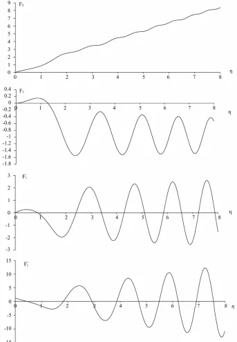
Solving Equations (24) and (25), under the following boundary conditions:

2 1 1 1 1 0

F F F F   (24)

 

1 2

1

0 0 , 0 0 0 0.01, 0 1.20

F F

 

     (26)

2 1 2 1 2 1

1 0 3

F F F F F F (25) Equations (24) and (25) are solved numerically apply-ing the shootapply-ing method coupled with Runge-kutta scheme using two groups of initial conditions illustrated

The obtained results are presented diagrammatically in (Figure 1).

Figure 1. Solution of (1 + 1)-dimensional dispersive long wave Equations (24) and (25) at A1 = B1 = B2 = 1.0. Where F1 refer to he surface velocity and F2 refer to the elevation of the water wave.

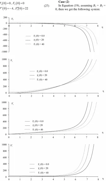
[image:4.595.128.471.211.705.2]

(5)

Case (1.2)

Also we solve Equations (24) and (25) under the fol-lowing boundary conditions:

 

1 2

1

0 0 , 0 0 0 4 , 0 2

F F

 

    

In addition to, the boundary conditions which illus-trated in the figures. The obtained results are presented diagrammatically in (Figure 2).

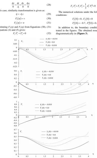
Case (2)

In Equation (19), assuming B1 = B2 = B3 = 0 and A1≠

0, then we get the following system:

[image:5.595.128.472.123.706.2]

2 (27)

Figure 2. Solution of (1 + 1)-dimensional dispersive long wave Equations (24) and (25) at A1 = B1 = B2 = 1.0. Where F1 refer to he surface velocity and F2 refer to the elevation of the water wave.

t

(6)

1

d d d d 0 0 0

x t v w

A

   (28)

In this case, similarity transformation is given as:

1

A x

 (29)

 

1

F  v (30)

 

2

F  w (31) Substituting F1(η) and F2(η) from Equations (30), (31)

into Equations (4) and (5) gives:

1 1 2 0

F FF (32)

2

2 1 1 2 1 1

1

0 3

F F F F  A F (33)

The numerical solutions under the following boundary conditions:

 

1 2

1 1

0 0 , 0 0 0 0.7 , 0 0.

F F

 

     5 (34)

[image:6.595.85.471.80.711.2]

In addition to, the boundary conditions which illus-trated in the figures. The obtained results are presented diagrammatically in (Figure 3).

Figure 3. Solution of (1 + 1)-dimensional dispersive long wave Equations (32) and (33) at A1 = 1.0. Where F1 refer to the sur-

(7)

Remark: Using MAPLE, we have verified all solutions we obtained by putting them back into the original NPDEs, WZ Equation (4) and (5). And it is worthy to point out that the new forms of solutions in Case (1), where the similarity variable _{  }_{x t} _0.5_t2

cannot be obtained by the generalized extended rational expansion method [22], and has not reported in the literature.

4. Conclusion

In this work, we have used the characteristic function technique to obtain similarity reductions of nonlinear partial differential Equations (4) and (5), for (1 + 1)-dimensional dispersive long wave equation (DLWE) in shallow water with uniform depth. The resulting system of non-linear ordinary differential with the associated boundary conditions is solved numerically using shooting method, coupled with Runge-Kutta scheme. The numerical solution was carried out for various values of the parameters of the equations to study different cases and illus- trate the effect of critical and special values on the per- formance of velocity and elevation of water wave.

REFERENCES

[1] M. Wadati, H. Sanuki and K. Konno, “Relationships among Inverse Method, Bäcklund Transformation and an Infinite Number of Conservation Laws,” Progress of Theoretical Physics, Vol. 53, No. 2, 1975, pp. 419-436.

doi:10.1143/PTP.53.419

[2] V. A. Matveev and M. A. Salle, “Darboux Transformations and Solitons,” Springer-Verlag, Berlin, Heidelberg, 1991.

[3] E. G. Fan, “Extended Tanh-Function Method and Its Ap- plications to Nonlinear Equations,” Physics Letters A, Vol. 277, No. 4-5, 2000, pp. 212-218.

doi:10.1016/S0375-9601(00)00725-8

[4] Y. B. Zhou, M. L. Wang and Y. M. Wang, “Periodic Wave Solutions to a Coupled KdV Equations with Variable Co- efficients,” Physics Letters A, Vol. 308, No. 1, 2003, pp. 31-36.

[5] P. J. Olever, “Applications of Lie Groups to Differential Equations,” Springer, New York, 1968.

[6] G. W. Bluman and S. Kumei, “Symmetries and Differen-tial Equations,” Springer, New York, 1989.

[7] H. Stephen,” Differential Equations: Their Solutions Us- ing Symmetries,” Cambridge University Press, Cambridge, 1990. doi:10.1017/CBO9780511599941

[8] N. H. Ibragimov, “CRC Handbook of Lie Group Analysis of Differential Equation,” CRC Press, Boca Raton, 1996.

[9] M. L. Wang, Y. B. Zhou and Z. B. Li, “Application of a Homogeneous Balance Method to Exact Solutions of Non- linear Equations in Mathematical Physics,” Physics Let- ters A, Vol. 216, No. 1-5, 1996, pp. 67-75.

doi:10.1016/0375-9601(96)00283-6

[10] E. G. Fan and J. Zhang,” Applications of Jacobi Elliptic Function Method to Special-Type Nonlinear Equations,” Physics Letters A, Vol. 305, No. 6, 2002, pp.383-392. doi:10.1016/S0375-9601(02)01516-5

[11] R. Seshadri and T. Y. Na, “Group Invariance in Engineer- ing Boundary Value Problems,” Springer-Verlag, New York, 1985. doi:10.1007/978-1-4612-5102-6

[12] M. B. Abd-el-Malek and M. M. Helal, “Characteristic Func- tion Method for Classification of Equations of Hydrody- namics of a Perfect Luid,” Journal of Computational and Applied Mathematics, Vol. 182, No. 1, 2005, pp. 105-116. doi:10.1016/j.cam.2004.11.042

[13] M. B. Abd-el-Malek and M. M. Helal, “The Characteris- tic Function Method and Exact Solutions of Nonlinear Sheared Flows with Free Surface under Gravity,” Journal of Computational and Applied Mathematics, Vol. 189, No. 1-2, 2006, pp. 2-21. doi:10.1016/j.cam.2005.04.038

[14] T. Y. Wu and J. E. Zhang, “On Modeling Nonlinear Long Wave,” In: L. P. Cook, V. Roytbhurd and M. Tulin, Eds., Mathematics Is for Solving Problems, Society for Indus- trial and Applied Mathematics, Philadelphia, 1996, p. 233.

[15] L. J. F. Broer, “Approximate Equations for Long Water Waves,” Applied Scientific Research, Vol. 31, No. 5, 1975, pp. 377-395. doi:10.1007/BF00418048

[16] D. J. Kaup, “Finding Eigenvalue Problems for Solving Nonlinear Evolution Equations,” Progress of Theoretical Physics, Vol. 54, No. 1, 1975, pp. 72-78.

doi:10.1143/PTP.54.72

[17] L. Martinez, “Schrodinger Spectral Problems with Energy- Dependent Potentials as Sources of Nonlinear Hamilto- nian Evolution Equations,” Journal of Mathematical Phy- sics, Vol. 21, No. 9, 1980, pp. 2342-2349.

doi:10.1063/1.524690

[18] B. A. Kupershmidt, “Mathematics of Dispersive Water Waves,” Communications in Mathematical Physics, Vol. 99, No. 1, 1985, pp. 51-73. doi:10.1007/BF01466593

[19] C. L. Chen and S. Y. Lou, “Soliton Excitations and Peri- odic Waves without Dispersion Relation in Shallow Wa- ter System,” Chaos, Solitons & Fractals, Vol. 16, No. 1, 2003, pp. 27-35. doi:10.1016/S0960-0779(02)00148-0

[20] M. L. Wang, “Solitary Wave Solutions for Variant Bous- sinesq Equations,” Physics Letters A, Vol. 199, No. 3-4, 1995, pp. 169-172. doi:10.1016/0375-9601(95)00092-H

[21] X. D. Zheng, Y. Chen and H. Q. Zhang, “Generalized Ex- tended Tanh-Function Method and Its Application to (1 + 1)- Dimensional Dispersive Long Wave Equation,” Physics Letters A, Vol. 311, No. 2-3, 2003, pp. 145-157. doi:10.1016/S0375-9601(03)00451-1