Journal of Modern Physics, 2012, 3, 85-101
http://dx.doi.org/10.4236/jmp.2012.31013 Published Online January 2012 (http://www.SciRP.org/journal/jmp)
Study of Decoherence of Elementary Gates Implemented
in a Chain of Few Nuclear Spins Quantum
Computer Model
G. V. López, P. López
Departamento de Física, Universidad de Guadalajara, Guadalajara, Mexico Email: [email protected]
Received October 20, 2011; revised November 26, 2011; accepted December 14, 2011
ABSTRACT
We study the phenomenon of decoherence during the operation of one qubit transformation, controlled-not (CNOT) and controlled-controlled-not (C2NOT) quantum gates in a quantum computer model formed by a linear chain of three
nu-clear spins system. We make this study with different type of environments, and we determine the associated decoher-ence time as a function of the dissipative parameter. We found that the dissipation parameter to get a well defined quantum gates (without significant decoherence) must be within the range of 4 104. We also study the behavior
of the purity parameter for these gates and different environments and found linear or quadratic decays of this parameter depending on the type of environments.
Keywords: Decoherence; Not Gate; Controlled-Not Gates; Controlled-Controlled-Not Gate; Nuclear Spin Chain; Quantum Computer
1. Introduction
Most of the ideal quantum insulated systems exist only in our mind, where one considers that environment has not interaction with the quantum system. However, in the real world the interaction of the system with the envi-ronment is almost unavoidable. In principle, one could study the unitary evolution of the whole system: quantum plus environment and their interaction, but this situation represents a many bodies problem which is unsolvable within any picture of the quantum mechanics. There are two approaches to attack this problem. The first one con-sists on to look for the phenomenological classical dissi-pative system and to get its associated Hamiltonian, then to proceed to do the usual quantization of the system [1, 2]. The other one, which it is more fundamental, uses the matrix density approach for the whole system and makes the trace over the environment variables [3-11]. The re-sulting density matrix is called “reduced density matrix”, and its associated non-unitary evolution equation is called “master equation”. This equation is also phe-nomenological one, and it has defined a dissipative and diffusion parameters which can (non Markovian process) or can not (Markovian process) depend on the time evo-lution of the system [3-17]. These parameters are respon-sible for the decay behavior of the non diagonal matrix elements of the reduced density matrix. This phe-
was used for studying sudden death of entanglement of two qubits. We will use this approach for our study of decoherence of several quantum gates during operation in a quantum computer model made up of a linear chain of three paramagnetic atoms with nuclear spin one half [31,34,36]. In this work, we are interested in determine the decoherence of a single qubit rotation, quantum con-trolled-not (CNOT), and quantum controlled-controlled- not (C2NOT) gates during their implementation on this
quantum computer model.
We describe the model and the Hamiltonian of our quantum system, and we must point out that, although this Hamiltonian will be time explicitly dependent, if we consider weak interaction between our system and the environment (the characteristic times of the quantum system are much longer than those of the environment) as a first approximation, the above mentioned Mark-ovian-Lindblad master type equation can be still used for our study [3,32,33]. On the other hand, even this model for solid state quantum computer has not been built yet, it has been very useful for theoretical studies about imple-mentation of quantum gates and quantum algorithms [34-36] which can be extrapolated to other solid state quantum computers [37-39].
2. Hamiltonian of the System
The Hamiltonian that describes the ideal insulated system of a linear chain of N paramagnetic atoms with nuclear spin one half inside the magnetic field
t
,B z
,,
, = cos , sin
B z t b t b (1)
where b, and are the amplitude, the angular
frequency and the phase of the RF-field, and B z
3
1 2
=0
2 N z z ,
k k k
J S S
represents the amplitude of the z-component of the mag-netic field, is given by (see [31,34])
1 2
=0 =0
= N 2 N z z
k k k k
k k
H B J S S
(2)where k represent the magnetic moment of the kth- nucleus, which it is given in terms of the nuclear spin as
= x, y, z S S S
k k k k , with
being the proton
gyro-magnetic ratio and j
k being the jth-component of the
spin operator, k represents the magnetic field, Equa-tion (1) valuated at the locaEqua-tion of the kth-nuclear spin ( k). The parameters
S B
=
z z J and J represent the cou-pling constant at first and second neighbor interaction. The angle between the linear chain and the z-component of the magnetic field is chosen as cos = 1 3
0
= ,
to eliminate the dipole-dipole interaction between the spins.
This Hamiltonian can be written as H W
1 2 3
0 1 2
=0 =0 =0
= N z 2 N z z 2 N z z
k k k k k k
k k k
H I J I I J I I
H (3) where H0 and W are defined as
(4)
and
1
=0
= ,
2
N
i t i t
k k
k
W e I e I
= S I
(5)
where we have used the relation , with the op-erator I written in terms of Pauli matrixes as I= 2. Here we have that: k k is the Larmor
fre-quency of the kth-spin,
= B z
=b
is the Rabi frequency, and = x y
k Ik Ik
I represents the ascend operator () or
the descend operator (). The Hamiltonian H0 is
di-agonal in the basis
N10
with k = 0,1 (zerofor the ground state and one for the exited state). The action of the spin operators on its respective qubit is given by z =
1 k 2k k
I k , k k k,0 ,
and
= 1
I
,1
k k = k 0 . The eigenvalues of
I H0 in this
basis are given by
1 1
1 0
1 =0 =0
3
2 =0
= 1 1
2
1 .
N N
k k k
k
N k k
N
k k k
E J
J
2
(6)
The elements of this basis forms a register of N-qubits with a total number of N registers which is the
dimen-sionality of our Hilbert space. The allowed transition of one state to another one is gotten by choosing the angular frequency of the RF-field, , as the associated angular frequency due to the energy difference of these two lev-els, and by choosing the normalized evolution time t
with the proper time duration (so called RF-field pulse). The set of selected pulses defines the quantum gate we want to study with this quantum computer.
3. System-Environment Interaction Models
Now, to deal with the non ideal situation where the effect of the environment is taken into account, we make use of the Lindblad type master equation for the evolution of the reduced density matrix
d
= , ,
d
i H L
t
(7)
where the first part on the right side denotes the usual von Neuman unitary evolution of the reduced density matrix, and the second term represents the Lindblad part (non unitary) evolution. This second term has different expression for different consideration of the system-en- vironment interaction. For the qubits interacting inde-pendently with the environment (case (A)), this term has the following form [30]
=1
1
= 2 ,
2 N
A i
j j j j j j j
L S S S S S S
i
(8)
G. V. LÓPEZ ET AL. 87
where j is the dissipative parameter associated to the jth-qubit.
For the pure dephasing interaction case, where the qubits independently dephase to their respective bath with a dephasing rate j, the Lindblad term is given by
=1
1
= N 2
B z z z
j j j j j
L S S
i
.z z z j j j S S S S
(9)
For the independent-qubit-correlated case (qubits in-teract with the environment collectively), the Lindblad operator is written as
, =1
1 =
2 N
jk C
j k k j k
L S S
i
2S Sj S Sj k
,
=
(10)
where one has that jj j is the decay rate of case (A). In this case, the decay of the state of a qubit has an effect on the other qubits.
For the qubit-correlated and dephasing case, with ij as the decay rate of the correlated dephasing, the Lind-blad operator is given by
=1
, =1
1
= 2
2
N
D z z z z z
j j j j j j
N
z z z z jk j k k j j j k
L S S S S
i
S S S S S S
i
.z j j
z z z z k j k S S
S S
(11) In this case, the decay of one qubit affects too the other qubits.
The dynamical system for each case for the reduced density matrix elements is deduced from Equation (7) as
d
= , ,
d
i H L
t
, = 1, , N (12)
where and represent the elements of the basis of the Hilbert space,
0 1
= N
and = N10 ,
and naming the ground state 0 0
= 3 N
as the first state of the system. In our case, one has that , the dimen-sionality of our Hilbert space is eight, and the explicit equations for the dynamical system of each case are given in the appendix.
4. Simulation Results
Our registers are made up of three qubits ABC
, , = 0,1 A B C
with , or written them with decimal notation,
1 = 000 , 2 = 001
2π MHz
= 100 , C
and so on (do not confuse with the type of environment). The parameters used for our simulation are taken from [36] and are given (in units of
) as
= 400,
= 10 , and = 0.4
A B
J J
= 200,
(13)
Using the assumption that the environment acts ho-mogeneously on the qubits, the damping parameter can be the same for each qubit, and the damping parameter for correlated cases at second neighbors can be one order of magnitude weaker that at first neighbors. Thus, the dissipative coefficients appearing for the cases (A), (B), (C), and (D) are taken of the following way
= = , = , = 1 ,
= 10, = 2, , = 1, 2,3
j jj jk
jk
k j
k j j k
(14)
where is the free common parameter which takes into account the interaction with the environment. The re-duced density matrix is then made up of 8 × 8 complex elements, and if the initial state is always taken as the ground state of the quantum state 1 = 000
11= 1
, this means that the initial reduced density matrix has the values
, = 1 i j .
and ij = 0 for
4.1. Single Qubit Rotation
We have selected the transition 000 (or in decimal notation: 1 2
π
) as an example of single qubit rota-tion (corresponding to the NOT quantum gate), and the NOT-reduced density matrix after a -pulse with reso-nant frequency CJ 2J2
= 1
would be such that
22 i j, = 2
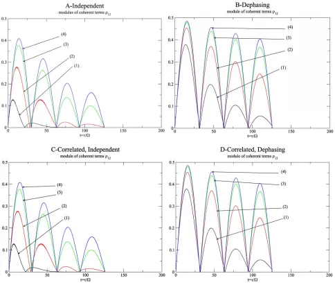
and ij = 0 for . In addition, we allow the system to run for almost two an a half -pulses more to see how the NOT gate evolves. Figure 1 shows the decoherence behavior (damping of the non diagonal matrix element 12
π
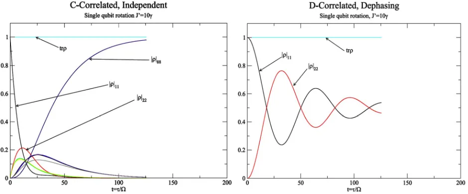
) for the cases (A), (B), (C) and (D), using different values for the damping parameter. In it, we can see a revival in the coherence with smaller am-plitude, which is due to the three and a half pulses ap-plied to the system. The effect of the environment is to reduce the amplitude of the coherent terms involved in the transitions, and to create new superposition of other states. Once enough time has passed, the destruction of the expected superposition will be absolute and new states take the entire probability of the system, like the state related to the element 88 in Figure 2.
The Figure 2 shows the behavior of the diagonal re-duced density matrix elements when dissipation is switched on, with = J10. Since one must have that
= 1tr , the damping of the matrix elements 11 and
22
G. V. LÓPEZ ET AL. 89
Figure 2. Diagonal elements of the reduced density matrix for =J10. To characterize the decoherence behavior of the off
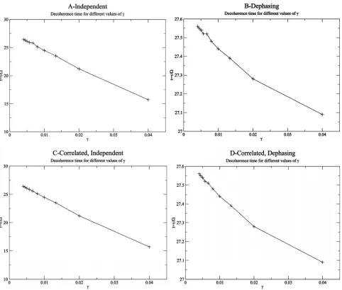
diagonal element of the reduced density matrix, assume that one defines the decay characteristic parameter as c as the time when the matrix element 12 has a value of
12 on the first pulse. Then, Figure 3 shows the
dependence of this characteristic parameter as a function of the dissipative parameter
max e
for our four cases. The behavior of this parameter as a function of the dissipative parameter can be fixed by a linear relation, c =
a b
b=
= 27.59 b
= 0
, where for the
inde-pendent cases (A) and (C), and for the dephasing cases (B) and (D).
=300.91,
a 27.57
= a 13.31,
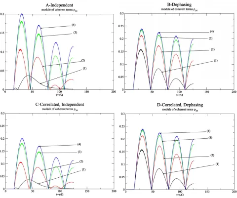
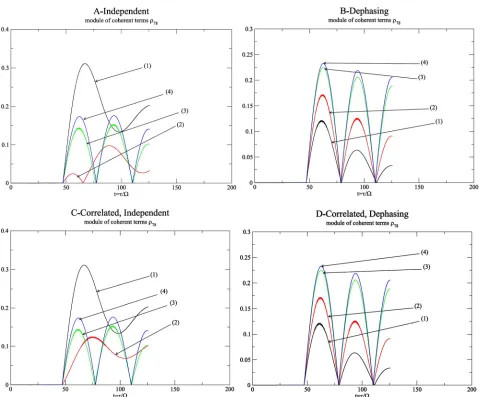
Other parameter which can help us to see the departure from the ideal ( ) behavior could be the distance
0 i
between the non diagonal matrix elements
12
of the ideal () and the dissipative cases (i, for ). Figure 4 shows the behavior of this distance for different values of
= A
,i
B , C , D indexed by (1) = J 10
, (2) =J30, (3) =J70 and (4) = J 100
. Of course, this distance increases as increases because the decoherence is taking place deeper. The maximum separation corresponds to the maximum on the coherence behavior as shown in Fig-ure 1.
4.2. Controlled-Not (CNOT) Quantum Gate
To get the CNOT quantum gate starting from the ground state 1 = 000 , one applies a π 2-pulse between this state and the state 3 = 010 , with resonant frequency
B
= J
, to get the superposition state
1 3
2π
. Then, one applies a resonant -pulse between the states
3 and 4 = 011 , with resonant frequency = C J 2 J 2
,
to get the final desired state
1 4
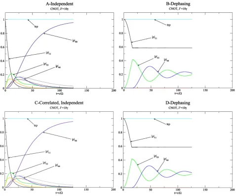
2 which meansthat the expected CNOT density matrix would be such that 11=14 =41=44 = 1 2, and all the other
ele-ments are equal to zero. In addition, one allows the sys-tem to have two and a half more resonant -pulses to have a better look of the CNOT behavior. Figure 5 shows the decoherence behavior (damping of the non diagonal matrix elements 34
π
) for the cases (A), (B), (C) and (D), using different the damping parameters. One observes from these figures that there is not significant difference between independent and correlated-independ- ent, and between dephasing and correlated-dephasing cases (similar behavior is observed for the other non diagonal matrix elements).
We note the peculiar behavior of the term 34 for the cases (A) and (C) of Figure 5, for a relatively high dis-sipation (labeled (1)). Before this superposition occurs, other elements of the density matrix have already been exited due to the interaction with the environment and the condition of Tr= 1. So, the other excited states
seems to have an important influence to slow the forma-tion of the superposiforma-tion, characterized by the term 34.
As the dissipation parameter goes weaker, a regular be-havior is observed. We can also see on Figure 5 that for short times, other states get exited besides the ones in-volved in the CNOT gate, therefore there are other states also overlapped with the states 3 and 4 . A revival in the superposition of 3 and 4 can be seen when enough of time has passed so that the other states excited by the environment have also went down (curve labeled with (1)). Figure 6 shows the diagonal reduced density matrix elements with =J10
= 1 tr
Figure 3. Characteristic time c as a function of dissipation parameter .
G. V. LÓPEZ ET AL. 91
Figure 4. Distance 0i between the ideal and dissipative coherent term 12 for different values of as a function
of time.
[image:7.595.59.539.317.718.2]JMP , one applies a
state
Copyright © 2012 SciRes. As we observed with the NOT quantum gate before, in
our simulations we observed for the CNOT gate that the dependence of the characteristic decay parameter c
with respect the dissipation parameter is linear for the non diagonal elements 13, 14 and 34, although
their parameters a and b have different values for differ-ent non diagonal elemdiffer-ents. However, these values are almost the same for the cases (A)-(C) and (B)-(D). In addition, the behavior of the distance ab 0i
B ,for cases for the non diagonal matrix elements is again very similar to that one found for the NOT quantum gate (Figure 5), that is, we observed and increasing of this distance as the dissipation gets stronger.
= A ,
i , C
D4.3. Controlled-Controlled-Not (C2NOT)
Quantum Gate
To get the C2NOT quantum gate starting from the ground
1 = 000 π 2-pulse between this state and the state 5 = 100 with resonant frequency = A J 2 J2 to get the superposition state
1 5
2. Then, one applies a resonant -pulse π between the states 3 and the state 7 = 110=
with resonant frequency B to get the desired superpo-sitional state
1 7
2π
. Finally, C2NOT operation
is achieved through a pulse between the state 7 and the state 8 , getting the state
1 8
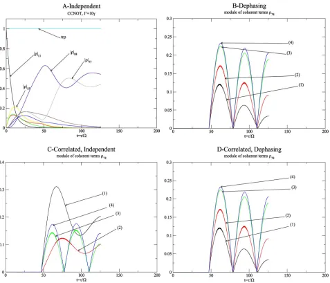
2. In addition, we allow the system to evolve for another al-most two an a half pulses to see the behavior of the C2NOT. The expected C2NOT density matrix would besuch that 11=18 =81=88 = 1 2 and all the other
elements equal to zero. Figure 7 shows the behavior of the non diagonal matrix elements 78 for the cases (A),
(B), (C) and (D), using different damping parameters. As in the CNOT gate, a similar strange behavior is seen for the coherent terms which appears later in the gate (57
[image:8.595.60.538.322.720.2]and 78) for the cases (A) and (C) at relatively high
G. V. LÓPEZ ET AL. 93
Figure 7. Non diagonal reduced density matrix element 78 for =J10 (1), =J 30 (2), =J 70 (3), and =J100 (4). dissipation parameter, that is, the state 8 is excited for
strong dissipation.
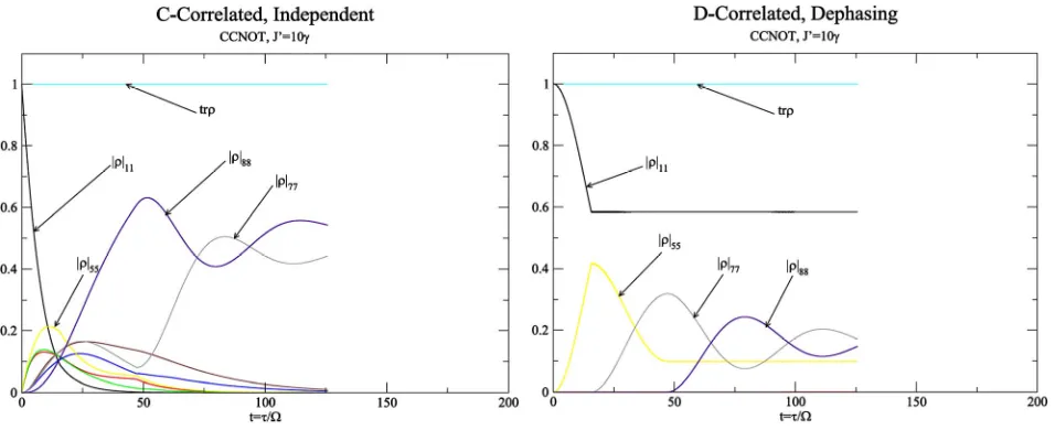
Figure 8 shows the diagonal reduced density matrix elements with =J10
= 1
tr
, for the four cases into consid-eration. Cases (A) and (C) showing the excitation of other diagonal elements to keep .
As for the NOT and CNOT quantum gates, in our simulation we observe a similar expected linear depend-ence of the characteristic decay parameter c with re-spect the dissipative parameter for the non diagonal elements, although the parameters a and b have different values for different non diagonal elements. The behavior of the difference a 0i
= 0
= 0
, between the non diagonal matrix elements of their ideal values and their dissipative values and for the cases
B , C , D = A ,i
is again similar as the other gates.
5. Purity Calculations
=
2P t tr
The purity function, , is a measure of how close a quantum system is from its description as a pure state quantum system and varies between 1 and 1d (d
the dimensionality of the density matrix). This function may decay with the decoherence since the system may move away from an initial pure state. Therefore, this function can be used to characterize the environment. Figure 9 shows the behavior of the purity for the CNOT gate using several dissipative parameters (the behavior of the purity is similar for the NOT and C2NOT quantum
Figure 8. Diagonal elements of the reduced density matrix for the C2NOT gate and
= 10
J .
G. V. LÓPEZ ET AL. 95
Figure 9. Purity for the CNOT quantum gate.
Figure 5, where the maximum values reached by the non diagonal matrix density elements are bigger for dephas-ing case than for independent case. Purity increases its value after the first decay for high damping values ( =J10
= 1
tr
) and for the independent case since for this value a particular state is exited (trying to keep ) as seen in Figure 6.
6. Conclusion
Within the Markov approximation for the study of quan-tum discrete system with environment, we have solved numerically the master equation for the reduced density matrix associated to our linear chain of three nuclear spin quantum computer interacting with the environment, and we have made the simulation of a particular single qubit transition (NOT gate), CNOT and C2NOT quantum gates
operating within this dissipative environment. Within the validity of this approximation, the coherence of these quantum logic gates have been determined, and we have calculated the associated decoherence time (using the first pulse applied to the system), c, as a function of a common dissipative parameter (all the dissipative pa-rameters appearing in the Lindblad part of the master equation were chosen proportional a single one), and it was found the expected linear dependence of this coher-ence time with respect this dissipative parameter, but with different decay rates for the non diagonal matrix elements and gates. The value of the dissipative parame-ter for the environment not to affect the performance of these quantum gates (within two cycles and a half after their formation) was found to be . We used the purity parameter to study its behavior of this chain of three nuclear spin system interacting with the environ-ment, and we have found an initial linear (or exponential) damping of the purity parameter for the independent case,
and an initial quadratic (or Gaussian) damping on its be-havior for the dephasing case, giving us an indication of strong (linear) or weak (quadratic) effect of the environ-ment in our system. For very strong dissipation, we found that purity may increase because, the condition
4
4 10
= 1
tr on the density matrix, sometimes implies strong
excitation of other state involved in the dynamics, caus-ing the system to try to return to a pure quantum state description.
REFERENCES
[1] G. López, M. Murgua and M. Sosa, “Quantization of One-Dimensional Free Particle Motion with Dissipation,” Modern Physics Letters B, Vol. 15, No. 22, 2001, pp. 965-742. doi:10.1142/S0217984901002750
[2] G. López and P. López, “Velocity Quantization Approach of the One-Dimensional Dissipative Harmonic Oscilla-tor,” International Journal of Theoretical Physics, Vol. 45, No. 4, 2006, pp. 734-742.
doi:10.1007/s10773-006-9064-9
[3] H.-P. Breuer and F. Petruccione, “The Theory of Open Quantum Systems,” Oxford University Press, Oxford, 2006.
[4] G. Lindblad, “On the Generators of Quantum Dynamical Semigroups,” Communications in Mathematical Physics, Vol. 48, No. 2, 1976, pp. 119-130.
doi:10.1007/BF01608499
[5] A. O. Caldeira and A. T. Legget, “Path Integral Approach to Quantum Brownian Motion,” Physica A, Vol. 121, No. 3, 1983, pp. 587-616. doi:10.1016/0378-4371(83)90013-4 [6] B. L. Hu, J. P. Paz and Y. Zhang, “Quantum Brownian
Motion in a General Environment: Exact Master Equation with Nonlocal Dissipation and Colored Noised,” Physical Review D, Vol. 45, No. 8, 1992, pp. 2843-2861.
doi:10.1103/PhysRevD.45.2843
Fisher, A. Garg and W. Zwerger, “Dynamics of the Dis-sipative Two-State System,” Reviews of Modern Physics, Vol. 59, No. 1, 1987, pp. 1-85.
doi:10.1103/RevModPhys.59.1
[8] W. G. Unruh and W. H. Zurek, “Reduction of a Wave Packet in Quantum Brownian Motion,” Physical Review D, Vol. 40, No. 4, 1989, pp. 1071-1094.
doi:10.1103/PhysRevD.40.1071
[9] A. Venugopalan, “Decoherence and Schödinger-Cat States in a Stern-Gerlach-Type Experiment,” Physical Review A, Vol. 56, No. 5, 1997, pp. 4307-4310.
doi:10.1103/PhysRevA.56.4307
[10] H. D. Zeh, “Toward Quantum Theory of Observation,” Foundations of Physics, Vol. 3, No. 1, 1973, pp. 109-116. doi:10.1007/BF00708603
[11] J. P. Paz and W. H. Zurek, “Environment-Induced Deco-herence, Classicality and Consistency of Quantum Histo-ries,” Physical Review D, Vol. 48, No. 6, 1993, pp. 2728-2738. doi:10.1103/PhysRevD.48.2728
[12] A. Rivas, A. D. K. Plato, S. F. Huelga and M. B. Plenio, “Markovian Master Equations: A Critical Study,” New Journal of Physics, Vol. 12, 2010, p. 113032.
doi:10.1088/1367-2630/12/11/113032
[13] F. Intravaia, S. Maniscalco and A. Messina, “Density- Matrix Operatorial Solution of the Non-Markovian Mas-ter Equation for Quantum Brownian Motion,” Physical Review A, Vol. 67, No. 4, 2003, p. 042108.
doi:10.1103/PhysRevA.67.042108
[14] S. Maniscalco and F. Petruccione, “Non-Markovian Dy-namics of a Qubit,” Physical Review A, Vol. 73, No. 1, 2006, p. 012111. doi:10.1103/PhysRevA.73.012111 [15] H.-P. Breuer, “Non-Markovian Generalization of the
Lindblad Theory of Open Quantum Systems,” Physical Review A, Vol. 75, No. 2, 2007, p. 022103.
doi:10.1103/PhysRevA.75.022103
[16] H.-P. Breuer, E.-M. Laine and J. Piilo, “Measure for the Degree of Non-Markovian Behavior of Quantum Proc-esses in Open Systems,” Physical Review A, Vol. 103, 2009, p. 210401.
[17] A. Rivas, S. F. Huelga and M. B. Plenio, “Entanglement and Non-Markovianity of Quantum Evolutions,” Physical Review Letters, Vol. 105, No. 5, 2010, p. 050403. doi:10.1103/PhysRevLett.105.050403
[18] W. H. Zurek, “Decoherence, Einselection, and the Quan-tum Origins of the Classical,” Reviews of Modern Physics, Vol. 75, No. 3, 2003, pp. 715-775.
doi:10.1103/RevModPhys.75.715
[19] W. H. Zurek, “Decoherence and the Transition from Quantum to Classical,” 2003, pp. 1-24.
[20] W. H. Zurek, “Decoherence and the Transition from Quantum to Classical,” Los Alamos Science, Vol. 27, 2002.
[21] H. D. Zeh, “There Is Not ‘First’ Quantization,” Physics Letters A, Vol. 309, No. 5-6, 2003, pp. 329-334.
doi:10.1016/S0375-9601(03)00209-3
[22] M. Zwolak, H. T. Quan and W. H. Zurek, “Quantum Darwinism in a Mixed Environment,” Physical Review
Letters, Vol. 103, No. 11, 2009, p. 110402. doi:10.1103/PhysRevLett.103.110402
[23] L. Mazzola, J. Piilo and S. Maniscalco, “Sudden Transi-tion between Classical and Quantum Decoherence,” Physical Review Letters, Vol. 104, No. 20, 2010, p. 200401. doi:10.1103/PhysRevLett.104.200401
[24] D. Solenov, D. Tolkunov and V. Privman, “Exchange Interaction, Entanglement, and Quantum Noise Due to Thermal Bosonic Field,” Physical Review B, Vol. 75, No. 3, 2007, p. 035134. doi:10.1103/PhysRevB.75.035134 [25] A. A. Slutskin, K. N. Bratus, A. Bergvall and V. S. Shumeiko,
“Non-Markovian Decoherence of a Two-Level System Weakly Coupled to a Bosonic Bath,” EPL, Vol. 96, No. 4, 2011, p. 40003. doi:10.1209/0295-5075/96/40003
[26] N. P. Oxtopy, A. Rivas, S. F. Huelga and R. Fazio, “Probing a Composite Spin-Boson Environment,” New Journal of Physics, Vol. 11, 2009, p. 063028.
doi:10.1088/1367-2630/11/6/063028
[27] D. Cohen, J. von Deft, F. Marquardt and Y. Imry, “The Dephasing Rate Formula in the Many Body Context,” 2009.
[28] Y. Hamdouni and F. Petruccione, “Time Evolution and Decoherence of a Spin-1/2 Particle Coupled to a Spin Bath in Thermal Equilibrium,” Physical Review B, Vol. 76, No. 17, 2007, p. 174306.
doi:10.1103/PhysRevB.76.174306
[29] Z. Gedik, “Spin Bath Decoherence of Quantum Entan-glement,” Solid State Communications, Vol. 138, No. 2, 2006, pp. 82-85. doi:10.1016/j.ssc.2006.02.004
[30] S. Das and G. S. Agarwal, “Decoherence Effects in In-teracting Qubits under the Influence of Various Environ-ments,” Journal of Physics B: Atomic, Molecular and Op-tical Physics, Vol. 42, No. 20, 2009, p. 205502. doi:10.1088/0953-4075/42/20/205502
[31] G. P. Berman, D. D. Doolen, D. I. Kamenev, G. V. López and V. I. Tsifrinovich, “Perturbation Theory and Nu-merical Modeling of Quantum Logic Operations with Large Number of Qubits,” Contemporary Mathematics, Vol. 305, 2002, pp. 13-41.
[32] A. Shabani and D. A. Lindar, “Completely Positive Post-Markovian Master Equation via a Measurement Ap-proach,” Physical Review A, Vol. 71, No. 2, 2005, p. 020101R. doi:10.1103/PhysRevA.71.020101
[33] I. de Vega, D. Alonso and P. Gaspard, “Two-Level Sys-tem Immersed in a Photonic Band-Gap Material: A Non-Markovian Stochastic Schrödinger-Equation Ap-proach,” Physical Review A, Vol. 71, No. 2, 2005, p. 023812. doi:10.1103/PhysRevA.71.023812
[34] G. V. López and L. Lara, “Numerical Simulation of a Controlled-Controlled-Not (CCN) Quantum Gate in a Chain of Three Interacting Nuclear Spins System,” Jour-nal of Physics B: Atomic, Molecular and Optical Physics, Vol. 39, No. 18, 2006, pp. 3897-3904.
doi:10.1088/0953-4075/39/18/019
[35] G. V. López, J. Quezada, G. P. Berman, D. D. Doolen and V. I. Tsifrinovich, “Numerical Simulation of a Quan-tum Controlled-Not Gate Implemented on Four-Spin Molecules at Room Temperature,” Journal of Optics B:
G. V. LÓPEZ ET AL. 97
Quantum and Semiclassical Optics, Vol. 5, No. 2, 2003, pp. 184-189. doi:10.1088/1464-4266/5/2/311
[36] G. V. López, T. Gorin and L. Lara, “Simulation of Grover’s Quantum Search Algorithm in an Ising-Nu-clear-Spin-Chain Quantum Computer with First-and- Second-nearest-Neighbor Couplings,” Journal of Physics B: Atomic, Molecular and Optical Physics, Vol. 41, No. 5, 2008, p. 055504. doi:10.1088/0953-4075/41/5/055504 [37] N. Y. Yao, et al., “Scalable Architecture for a Room
Temperature Solid-State Quantum Information Proces-sor,” 2002.
[38] S. Lloyd, “A potential Realizable Quantum Computer,” Science, Vol. 261, No. 5128, 1993, pp. 1569-1571. doi:10.1126/science.261.5128.1569
[39] F. H. L. Koppens, et al., “Driven Coherent Oscillations of a Single Electron Spin in a Quantum Dot,” Nature, Vol. 442, 2006, pp. 766-771.doi:10.1038/nature05065
Appendix
17 17
27 37 57 13 15
18
= 2 2
2 2
A B i t
i t
vN j j
e e
The evolution equation for the density matrix elements are given from Equation (12) by
d 1
= , , , = 1, ,8.
d i H L t i
(X1)Making the following definition
1 1
= , and = ,
vN H L
i i
51 15 (X2) one getsVon Neuman (vN) Part
21 31 11 12 13 = 2 2 i t i t vN e e (V1)
12 12
22 32
= 2 2
2 C
i t
vN j j
e
52 11
14 16
2 i t
e
13 1333 53 11
14 17
= B
vN j
(V2)
23 2 2 i t i t e e
(V3)
1454 12 13
2 14 24 34 18 = 2 2 2 B C i t i t
vN j j
e e
(V4)
15 55 11 16= A 2 2
vN j j
15 25 35 17 2 2 i t i t e e
16 1656 12 15
= A C
vN j
(V5) 26 36 18 2 2 i t i t e e (V6) (V7)
18 1828 38 58 14 16 17
= 2
A B C i t vN
e
42 62 21
22
12 26 24
= 2 2 i t i t vN e e (V8)
(V9)
23 2343 63 21
13 24 27
= 2 2
2 2
B C i t
i t
vN j j
e e
(V10)
24 44 64 22 23
24 14 28 = 2 2 i t B i t vN e e
(V11)
25 2545 65 21
15 27 26
= 2 2 A C i t i t vN e e (V12)
26 2646 66 22 25
16 28
= 2 2
2 2
A i t
i t
vN j j
e e (V13)
27 2747 67 23 25
17 28
= 2 2
A B C i t i t vN e e (V14)
28 2848 68 24 26 27
18
= 2 2
2 2
A B i t
i t
vN j j
43 33 13 = 2 2 i t i t vN e e
73 31 34 37 (V16)
34 44 74 14 = 2 2 2 C i t i tvN j j
e e
34 32 33 38 2
56 5666 76 52 55
16 58
= 2 2
2 2
C i t
i t
vN j j
e e
(V17)
35 75 31 37 36 2 j 35 45 ( ) 15 = 2 2 2 A B i t i t vN j e e
32 35 38
vN =
(V18) 36 36 46 76 16 2 2
A B C i t i t e e
(V19)
47 77 17 2 2 i t i t e e
37 37 33 35 38= A 2 2
vN j j
(V20)
48 78 18 2 2 i t i t e e
34 36 37
38
38= A C
vN j
84 4244= 2
i t
vN e
43 34 48 (V21) 242 i t
e
45 47 46
45= A B C
i t vN (V22)
85 41 25 35 2 2 i te
e
(V23)
46 42 45 36 48= 2 2
2
A B i t
vN j j
e
46 ( ) 86 ( ) 262 i t
e
43 45 37 48
47
47( ) 87 = 2 A C i t vN
e
(V24)
( )
27
2e i t
(V25)
48 4888 44 46 47
38
= 2 2
2
A i t
vN j j
e
28
2 i t
e
51 57 56
65 75 55 ( ) 15 = 2 2 i t i t vN e e (V26) (V27)
(V28)
= 2 i t
vN e
57 67 77 53 55
57
17 58
2
B i t
e
(V29)
58 5868 78 54 56 57
18
= 2 2
2 2
B C i t
i t
vN j j
e e (V30)
86 62 65
66
26 56 68
= 2 2 i t i t vN e e
(V31)
67 6787 63 65
27 57 68
= 2 2
2 2
B C i t
i t
vN j j
e e
(V32)
68 6888 64 66 67
28 58 = 2 2 B i t i t vN j e e (V33)
87 73 75
77
37 57 78
= 2 2 i t i t vN e e
(V34)
78 7888 74 76 77
38 58
= 2 2
2 2
C i t
i t
vN j j
e e (V35)
84 86 87
88
48 68 78
= 2 2 i t i t vN e e
(V36)
Lindblad Part
dent Case A: Indepen
= , ,
2 .
i i i i i i i i A B C
= 2 s s sss s
11 11 12 12 = ,= 2 ,
A B C A B C
(A1)
13 13
14 14
= 2 ,
= 2 2 ,
A B C A B C
(A2)
15 15
16 16
= 2 ,
= 2 2 ,
A B C A B C
(A3)
G. V. LÓPEZ ET AL. 99
17 18 2 ,2 2 ,
C C
16 16 17 17
18 18
= , = ,
= ,
A C A B
A B C
17 18 = 2 = 2 A B A B
22 11 23 = , 2 , C C (A4)
2223= 2
A B A B = 2
24 13 25 , 2 , C C (A5) 2425= 2
A B A B
26 15 27 ,2 2 ,
C C
26= A2 B
(A6)
27= A2 B
28= A2 B
2
28 C 17 (A7)
33 11 34 12 = , , B B (A8)
33 A C
34 = A C2
35 = A2 B
35 36 2 ,2 2 ,
C C (A9)
36 = A2 B
37 = 2
= 2 A C
37 15 38 16 , 2 , B B (A10)38 A C
22
3345= ,
2 2 ,
C C
44 44
45= 2
A B A B (A11)
46 35 47 25 2 , 2 , C B (A12) 46 47 = 2 = 2 A B A C 26 C 37
(A13)
48= A2 48 B
55 A 11 B
55 56 = ,= 2 ,
C C
(A14)
56 A 12 B
57 58= 2 ,
= 2 2 ,
A B C A B C
(A15) 57 13 58 14
66
556768 57
= ,
= 2 2 ,
, C C C (A16) 66 22 67 23
68= 24 2
A B A B A B 55 77 56 78 = ,
= 2 ,
C C (A17) 77 33 78 34 A B A B
88 A 44 B
66 77
= C .
(A18)
z z 2 z z z z
,i i i i i
(A19)
Case B: Pure Dephasing
= , ,
i i i A B C
= s s s s s s
= 0, = 1, ,8
ii i
13 15 15 , = , B A (B1)
12 12 13
14 14 = , = = , C B C
(B5)
(B8)
23 23 24 24
25 25 26 26
= , = ,
= , = ,
B C B
A C A
(B13)
27 27 28 28 = , = ,A B C A B
34 34 35 35
36 36
= , = ,
= ,
C A B
A B C
(B15)
37 A 37 38 A C 38
(B19)
= , = ,
(B21)
45= A B C 45, 46= A B 46,
(B24)
47 = A C 47, 48 = A 48,
56 56 57 57
58 58 = , = , = , C B B C (B26)
(B30)
67 = B C 67, 68= B 68,
(B33)
78= C 78,
Case C: Independent Correlated
(B35)
The Lindblad expression is given by
, = , ,
= jk2 j k 2 k j j k
j k A B C
s s s
ss s
where ii=i is as the case A, and it can be written as
where the the independent part A corresponds to the case
= A ind C corr,
A above and the correlated part is
= , ,
2 .
jk j k k j j k j k A B C
= 2
C corr
s s s
s s s
11= 18= 0,
c c
(C1)
12 15 13
13 15 12
= 2 2 ,
= 2 2 ,
c CA CB c BA BC
(C3)
14 16 17
15 13 12
= 2 2 ,
= 2 2 ,
c BA CA c AB AC
(C5)
16 14 17
17 14 16
= 2 2 ,
= 2 2 ,
c AB CB c AC BC
(C7)
22 52 25
32 23
= 2 2
2 2 , c AC CA BC CB (C9)
23 25 53
33 11 22
= 2 2
5434 122
2
BC 35
, (C11)24 26 27 = 2 2 2 c BA AC CA BC 25 23
55 11 22
= 2 2 2 c AB AC 2 ,
(C12)
56 12
27 2 2 , 26 24 36 2 AB AC BC CB
= 2 2
c
1315 2624
2 2 , = 2 c (C13) 27 57 37 2 AC BC
14 38 16 2 2 , 53 35 32 23 2 2 , BA CB 28= 2 58
c
AC
(C14)
BC2
33 = 2
c
AB
(C15)
BC2
3624 13
2 2 , BA
33 25, CB 34 = 2 54
c AB (C16) 37
CA2 CB2
35 = 2 55 2 11
2 2 c AB (C17) 32 AC
12 34 15 37 2 2 ,
13 27 2 2 2 , AC CB (C18)36 = 2 56
2 c AB 26 CB
37 57 36 = 2 2 c AB BC(C19) 34
14 17 2 , 64 46
47 32 23
2
2 2 ,
BA BC CB
(C20) 38 58 28 = 2 2 2 c AB CB
(C21)
44= 2
2 c
AB CA
AC274
43 42 ,
22 44 25 2 2 2 , (C22)
45 65 21
75 31
= 2 2
2 2 c AB AC c
(C23)
76 32 AC46= 2 66
2 2 AB 47 CB
(C24)
23 33 44 35 2 2 2 , 47 67 77 46 = 2 2 2 c AB AC BC (C25)
24 34 27 2 2 , CB 48 68 78 36 = 2 2 c AB AC BC (C26)
55 53 35
52
= 2 2
2 2 c AB BA AC CA 25, (C27)
56 54 36
26 15
= 2 2
2 2 2 , c
AB BA CA
CB 57
(C28)
57 37 15 54
27 56
= 2 2 2
2 2 , c BA AC CA BC
(C29)
58= 2 38 2 16 2 28 2 17 ,
c
BA CA
(C30)
66 64 46 52
76 67
= 2 2
2 2 ,
c
AB BA AC BC CB
CA 25
(C31)
67 47 25 64 53
77 55 66
= 2 2 2 2
2 2 ,
c BA AC BC (C32)
68 48 26 54
27 78 56
= 2 2
2 2 ,
c BA AC CA BC (C33)
77 53 35 74 47
76 67
= 2 2
2 2 ,
c
AB BA AC CA BC CB (C34)
78 54 36 48 37
68 57
= 2 2
2 2 ,
c
AB BA CA
CB (C35)
88 64 46 74 47
76 67
=
.
c
AB BA AC CA BC CB (C36)
Case D: Dephasing Correlated The Lindblad term is
, = , ,
= z z 2 z z z z ,
ij i j j i i j i j A B C
s s s s s s
with ii being the i as the case B (Pure dephasing), and one has ij =ji. This expression can be written as
= B d
e B
wher is the Lindblad term of the case B (pure dephasing), and the other term is given by
= , ,
2 ij i j 2 j i 2 i j i j i j A B C
=
d z z z z z z z z
s s s s s s s s
14 14 15
=
d
BC
(D1)
16 16 17 17
18 18
= 2 , = 2 ,
= 2 ,
d d
AC AB
d
AB AC BC
11 0, 12 = 0, 13 = 0,
= 2 , = 0,
d d d d
(D2)
22 23 23 24
25 25 26
= 0, = 2 , = 0,
= 2 , = 0,
d d d
BC d d AC
(D3)
G. V. LÓPEZ ET AL. 101
AC BC
27, 2728 28
= 2
= 2 ,
d
AB d
AB
35 36
= 2 ,
,
d AB
(D4)
33 34
36
= 0, = 0,
= 2
d d
d
AB AC BC
35
d d
38
= 2 AC ,
(D5)
37 = 0, 38
(D6)
C BC
45,
= 0,
d
44
45= 2
d
AB A
(D7)
46 46 47
48
= 2 , = 2
= 0,
d d
AB AC
d
47,
55 56 57
58 58
= 0, = 0, = 0,
= 2 ,
d d d
d
BC
66d = 0, 67d = 2 BC 68, 6d = 0
77d = 0, 78d = 0,
(D11)
88= 0.
d
(D8)
(D9)
8 , (D10)