doi:10.4236/am.2011.210173 Published Online October 2011 (http://www.SciRP.org/journal/am)
High Accuracy Arithmetic Average
Discretization for Non-Linear Two Point
Boundary Value Problems with a Source
Function in Integral Form
Ranjan K. Mohanty, Deepika Dhall
Department of Mathematics, Faculty of Mathematical Sciences, University of Delhi, Delhi, India E-mail: [email protected]
Received June 17, 2011; revised June 30, 2011; accepted July 6, 2011
Abstract
In this article, we report the derivation of high accuracy finite difference method based on arithmetic average
discretization for the solution of , 0 < x < 1, 0 < s < 1 subject to natural boundary
conditions on a non-uniform mesh. The proposed variable mesh approximation is directly applicable to the integro-differential equation with singular coefficients. We need not require any special discretization to ob-tain the solution near the singular point. The convergence analysis of a difference scheme for the diffusion convection equation is briefly discussed. The presented variable mesh strategy is applicable when the inter-nal grid points of the solution space are both even and odd in number as compared to the method discussed by authors in their previous work in which the internal grid points are strictly odd in number. The advantage of using this new variable mesh strategy is highlighted computationally.
1
0
, , , d
uF x u u
K x s sKeywords: Variable Mesh, Arithmetic Average Discretization, Non-Linear Integro-Differential Equation,
Diffusion Equation, Simpson’s 1
3Rd Rule, Singular Coefficients, Burgers’ Equation, Maximum
Absolute Errors
1. Introduction
We consider the non-linear differential equation with a source function in integral form:
1
0
, , , d , 0 , 1
uF x u u
K x s s x s . (1) The two point boundary conditions associated with (1) are given by:
0 0,
1u u 1 (2)
where 0, 1 are finite constants. We assume that K(x, s) is a real valued function of both variables in the range 0 ≤x, s ≤ 1.
Let
1
0, d
I x
K x sand
, ,
, ,
F x u u I x G x u u
Then we may re-write (1) as
, ,
, 0 1uG x u u x (3)
Keller [1] has given the conditions under which the differential Equation (3) together with the boundary con-ditions (2) has a unique solution. We assume that these conditions are satisfied in the problem that we are con-sidering. In addition, we assume that
6
0,1u x C
and
, 4
0K x s C ,1 .
Many physical problems from fluid mechanics, fluid dynamics, elasticity, magneto-hydrodynamics, plasma dynamics, oceanography, biological model, boundary layer theory, …etc are described mathematically by non- linear integro-differential equations. Davis and Rabi-nowitz [2], Philips [3], Linz [4], Lakshmikantham and
Rao [5], Atkinson [6], and Agarwal and O’Regan [7] have discussed various techniques for numerical integra-tion and methods for approximate soluintegra-tion of integro- differential equations and their applications to various physical models. Most of the nonlinear differential equa-tions cannot be solved analytically. So it is required to obtain efficient numerical methods. Jain et al. [8] have discussed variable mesh methods for the solution of two point nonlinear boundary value problems; however, their methods are not applicable to differential equations with singular coefficients. In recent years, Mohanty et al. ([9- 12]) have discussed a family of third order variable mesh methods for the solution of two point non-linear bound-ary value problems and obtained convergent solution for singular problems. More recently, Mohanty and Dhall [13] have proposed a three-point third order variable mesh method for the solution of non-linear integro-dif- ferential Equation (1), which is applicable only when the internal grid points of the solution region are odd in number. In this paper, we propose an efficient third order variable mesh method based on arithmetic average dis-cretization for the solution of non-linear integro-differ- ential Equation (1), which is applicable when the internal grid points of the solution region are both odd and even in number. In next section, we give mathematical details of the method. In Section 3, we discuss the application of the proposed method to an integro-differential equation with singular coefficients and study the convergence analysis. In Section 4, we give numerical results to jus-tify the utility of the proposed new strategy. Final re-marks are given in Section 5.
2. Mathematical Details of the
Discretization
We discretize the solution region [0,1] with the non- uniform mesh such that 0x0x1xN11
1
N
. Let 1 1 be the variable mesh size in x-di- rection, where k k k 0 . Grid points are given by
h x x
i
0 1
k
0 1
i k
k
x x h
, i1 1
N1. The mesh ratio is
1
0k hk hk
. When k 1, then it reduces to the
constant mesh case. The off-step points are defined by 1
2 2
k k k k
h
x x
and 1
2 2
k k k
h
x x
etc. Let the exact solution of u(x) at the grid point xk be denoted by
and u be the approximate value of .
kU u xk k k
Let us construct a numerical method for evaluating the
U
integral
10
d
x x
, where
x is a real-valued con-tinuous function in [0,1].
Using the derivation technique discussed in [13], we obtain a fourth order accurate integral formula based on Simpson’s 1
3rd rule (see Evans [14]).
1
1 2
1
1
d 4
6 0,1, 2,
k
k
x
k
k k x
h x x
k N
k ,
(4)
where k
xk , k1
xk1
xkhk1
,1
1 1
2 2 2
k k
k k
h
x x
, etc.
Then on the variable mesh the value of the integral
1
2
1
0 1
1
0
1
1 1
0 2
d d d
4 6
N
N x
x x
x x x
N k
k k
k k
d
x x x x x x x
h
x
(5)
can be found by the repeated application of (4).
Now we discuss the third order numerical method based on arithmetic average discretization for the differential Equation (3).
At the grid point xk, we denote
, ,
k k k k k
UG x U U G (say),
and
,
k k
k k
x x
G G
u u
.
Using Taylor expansion, from (3), we obtain
1 1
2
5
1 1
2 2
1
1
,
3 2
1
k k k k k
k k k
k k
k k
k
U U U
h
G G G O
k
h (6)
We need the following approximations:
1 1
2
1
2 k k k
U U U
, (7a)
1 1
2 1
2 k k
k
U U U
, (7b)
1 1
2 1
k k
k
k k
U U
h
U
, (7c)
1 21
k k
k k
U U U
h
1245
1
2
2 11
1 1
k k k k
k k k
U U U
h
2 2
3
1 1
2 2
3 ,
24 1
k k
k k k k k
k k
k
h
G G U U O h
(9a) kUk , (7e)
and let
2
3
1 1
2 2
3 ,
24 1
k
k k k k k
k k
k
h
G G U U O h
(9b)
1 1 1 1
2 2 2 2
, ,
k k k k
G G x U U
. (8)
From (9a) and (9b), it follows that It is then easy to see that
2
2
31 1
2 2
2 1 1 3 3 ,
2 24
IV
k k
k k k k k k k k k k k
k k
h h
G G U U U U U O h
1 (10a)
2
2
31 1
2 2
1 1 3 3
2 24
IV
k k
k k k k k k k k k k
k k
h h
G G U U U U O h
, 1 (10b)
2 3
2 ,
k k k k k k
U U ah U O h
Now, let 1, (12a)
2
1 1
2 2
k k k
k k
U U ah G G
, (11a)
2
3
3 1 ,
6
1
k
k k k k k k
k
h
U U b U O h
(12b)
1 1
2 2
k k k
k k
U U bh G G
, (11b) Further, we define
, ,
k k k k
G G x U U (13)
where “a” and “b” are parameters to be determined. With the help of (10a) and (10b), from (11a) and (11b),
we obtain and with the help of (12a) and (12b), it follows that
2
2 3
2 3 1
6
k
k k k k k k k k k k k
h
G G ah U b U O h , 1 (14)
Then at each internal grid point xk, the differential Equation (3) is discretized by
1 1
2 1
1
2 2
1
1 ,
3 2
k k k
k k k k k k k k
k k
h
U U U G G G T k
1 1 N (15) where
5k k
T O h , provided k 1.
Now with the help of the approximations (9a), (9b)
and (14), from (6) and (15), we obtain the local trunca-tion error
4
2 2
1 3 1 8 1 6 1 ,
72
k
k k k k k k k k k k k k k k
h
T a U b UO h5
1 (16)The proposed numerical method (15) to be of
3 k O h , the coefficient of in (16) must be zero and we obtain the values of parameters4 k
h
tial equation
1
2 2
0
, d ,
0 , 1
d u du
A r B r u f r K r s dr
dr
r s
s(17)
1 2
1 2
, ,
8 6(1
k k k k
k
a b
)
where A r
,B r
2r r
and the local truncation error given by (16) becomes
5k k
T O h , k 1. . For = 1 or 2, the
equation above represents cylindrical or spherical prob-lem, respectively. Replacing the variable x by r and ap-plying the formula (15) to the integro-differential
equa-3. Application to Singular Problems
2
1 1 1 1 1 1 1 1
2 2 2 2 2 2
1 1 1 1 1 1
2 2 2 2 2 2
1
3 1
0, 1 1 2
k k
k k k k k k
k k k k k k
k
k k k k k k k
k k k k k k
h
U U U A U B U f I
A U B U f I A U B U f I T k
N
(18)
where
,
,
,
k k k k k k k k
U u r A A r B B r f f r ,
1 2 1
0 1
1
0
, d , d
N
N
r r r
k k k k
r r r
I I r K r s s K r s s
,
2
21 1 1 1 1 1 1 1 1 1 1 1
2 2 2 2 2 2 2 2 2 2 2 2
1 8
k k k k k
k k k k k k k k k k k k
h
U U A U B U f I A U B U f I
,
2
1 1 1 1 1 1 1 1 1 1 1 1
2 2 2 2 2 2 2 2 2 2 2 2
1 6 1
k k k k k
k k k k k k k k k k k k
k
h
U U A U B U f I A U B U f I
,
nd
eme (18) is directly applicable to sin-gu
he scheme (18), we use the fol-lo
a
5k k
T O h . te that the sch No
lar problem (17) and do not require any fictitious points outside the solution region to compute the scheme. The scheme is also applicable when the internal grid points of the solution region are both even and odd in number as compared to the scheme discussed by Mo-hanty and Dhall [13] in which the internal grid points are strictly odd in number.
For convergence of t wing approximations:
2 2
3 1
2 2 8
k k k k
k k k
k
h h
k
I I I I O
h , (19a)
2
3 1
2 2 8
k k
k k k
k
h h
k
I I I I O h
, (19b)
2 2
3 1
2 2 8
k k k k
k k k
k
h h
k
A A A A O
h , (19c)
2
3 1
2 2 8
k k
k k k
k
h h
k
A A A A O h
. (19d)
Similarly, we can define the approximations for 1 2 k
B
and 1 2 k
f
, where
, ,
, , , e
k k k k
k k
d d
A A r B B r
dr dr
d K
f f r K r s
dr r
tc
and
1
1 2
0 1
1
0
, d
, d , N
N
k k k
r r r
k
r r r
d
I I r K r s s
dr
K r s s
1
1 2
0 1
1 2
2
0
, d
, d . N
N
k k k
r r r
k
r r r
d
I I r K r s s
dr
K r s s
Using the approximations (19) in (18), neglecting high order terms and simplifying we get the modified scheme in compact form
1
11
1 0
k k k k k
k k k k
k
sub U diag U
sup U T
(20)
where
2
2
2
2 2
2 3
6 3 2 8
6 2
1
2 72
1 1
, 48
k k k k k k
k k k k k
k k k
k k
k k k k k
k k k k
k k k k k k k
h h h h
sub A A A A
h h
B B
A h
A h A B
A B h
1247
2 2 2 2 2
2 2 2 2 3
1 1 1 1 1 1
6 6 4 3 4 8
1 1 1 1
1 2 ,
36 2 48
k k k k k k k k k k k k k k k k
k k k k k k
k k k k k k k k k k k k k
k k k
h B
h h h h B
diag h A A A B
A h B h B h
A A
kB hk k
2 2 2 2
2 2 2 3
6 3 2 8 6 2
1 1
2 ,
72 48
k k k k k k k k k k k
k k k k k k k
k k k k k k k k k k
k k k k k
h h h h h h
sup A A A A B B
1
A h A
A A B h
B h
2 2 2
2 2
2
1 1
3
6 4
1 1
1 ,
12 4
k k k k
k k k
k k k
k k k k k k
k k k k
B h
h
f I
A h
h f I h f I
k k k
and
In
e boundary values 5 .k k
T O h
corporating th U00, UN11, can be writ-the difference Equation (20) in ma
ten as
(21) where
trix form
DP U
T
hk 0
k,1 k, 1
D
are tri-diagonal matrices of order
and P = [subk, diagk, supk] N and
1 1
0, , ,2 1,
1
1 TN N N
sub sup
,
T1, 2, , N
U U U , hk T T1, ,2
0,0, ,0
T 0 are vectors.
U T
,T
T
1, , ,2
T N
u u u
u U which satisfies
N and
Let
DP u
0 (22) Let ek ukUknce of 1, ,e2 U
btracting (21) f
be the discretization error (in the abse round of errors) at the grid point rk and
be the error vector.
), we obtain the error equa-tion
,
TN
e
E u
Su rom (22
e
DP E
T
hk (23) Let Ak G1, Ak G2, Ak G3, Bk H1, Bk H2,3 k
B H , where G1, G2, G3, H1, H2 and H3 are some positive constants. If pi, j be the (i, j)th-element of P, then
k k
hk 2
3 , 1 1
1,G O h k N
(24a) 2
, 1 1 1
1 1 2
6 6
k
k k k k
h
p G
2
2 1
kh Gk H
2
2
3
, 1 1 2 1 1
1
1 2 , 2 1
6 6
k k k
k k k k k
h
p G h G H G O h k
Thus for suffic , the matrix (D r-educible (see V oung [16]).
,
N (24b)
khk
iently small hk arga [15] and Y
+ P) is i r
Let Sk be the sum of elements of the kth-row of (D + P), then
2
1 2
2
31 2 2 3 ,
6 6 6
k k
k k
k k k k k k k k k k
h h
S A h A B A O
1
h k (25a)
2
2
1 2
2
1 1 2 3 2 3 ,
6 6 6
k k
k k
k k k k k k k k k k k
h h
S A h A B A O h k N
1
3 , 2 1
1. 2k
k k k k k
h
S B O h k N (25c) 2
Let 1* 1min k k N
G A
, 1
1maxk N k
G A
, 1* 1min k
k N
H B
,
1 1max k k N
H B
, then 0 < G1*≤ G1 ≤ and 0 < H1*≤ H1≤
1
G
1
H.
It is straightforward to show that for sufficiently small hk, (D + P) is Monotone (see Varga [15] and Young [16]). Hence (D + P)–1 exists and (D + P)–1≥0.
From error Equation (23), we have
1
k
h
E D P T
for sufficiently small hk, it is easy to show that (26) Thus
2 3
2 1*, 16 k k k h H k
, (27a) k
S
3 2
2 1*,6
k
k k k
S H kN, (27b)
h
21 hk , 2 1 S H1* k N
2
k k k 1. (27c)
Since
1 i k, 0
D P and
,1 i k
k
D P 1 . Sk 1,N
1 1
i N,
hence
1
2 , 1* 1 6 , 1 2 3 i k
k k k k
k
S H h
D P (28a)
1
2 , 1* 1 6 , 3 2 i k
k k k k
k N
S H h
D P Further, (28b)
1 N 1 2 2 1*1 2 ,
min 1 1 1
k k k k
k N S ,
2 1
i k
k H h
i N
D P(29
For any matrix M, we define
)
, 1 i k k m
, 1 max N i N Mwhere mi k, is the (i, k)th-element of M and
1 max k i i N h T T .With the help of (28a), (28b), (29), from (26), we ob-tain
5 2 1* 36 1 1 1
2 3 3 1 3 2 k
k k k
k k k O h H h O h E (30 This establishes the third order convergence of the
method (20).
merical Results
In this section, we consider another ne method for the solution of non-linear in Equation (1) as
)
4. Nu
w variable mesh tegro-differential
1 1 2 1 1 2 22 3 k 3 k
2
4
1 1
1
1 2 2
1 2 2
, 1 1
k k k k k
k k
k k
k k k
k
U U U
h
F F
h
2 2
2 3 k 3 k
k
I I O h
N (31) where k
1 1 1
2 2 2 2
, ,
k k k k
F F x U U
1,
1 1, 1, 1
F F x U U ,
2 2 2 2
k k k k and
1
, d ,
1 1
.k k k
0 s
I I x
K x s s k N The approximations associated with 1
2 k
F
defined by (7a)-(7d). The order of accuracy of the method (31) is of
are already
2 k O hwe replace the i
. For evaluating the integral associated with (31), ntegral by the trapezoidal rule (see Evans [14]).
1 1 2 0 1 1 0 1 1 0d d d
2
N
N x
x x
x x x
N k
k k k
d
x x x x x x x
h
x (32)In this section, we have solved two benchmark prob-lems using the proposed method described by equation (15) and compared our results with those obtained by using the variable mesh method discussed by Mohanty and Dhall [13] only for the cases whe internal grid points are odd in number. We have also puted our
ts using uniform mesh (when
n com
resul k 1
y be ob
) for all values e boundary conditions ma tained using the exact solution as a test procedure. The linear difference equation has been solved using a tri-diagon lver, whereas non-linear difference equations have been solved using the Newton-Raphson method (see Kelly [17] and of N. Th
1249
Ev aph
the iterations were stopped when absolute error tolerance
1,
ans [18]). While using the Newton-R son method,
≤10–12 was achieved.
The unit interval [0,1] in the space-direction is divided into (N + 1) points with
0x0x1xN xN1
where
1
k k k
h x x
and
1
0, 1, 2, , .k hk hk k N
We may write
1 0 1 1 1 0
1 1 1 1 2 1 2
1 N N N N N
N N N
x x x x x x x x
h h h h
1 1. (33) For simplicity, we consider
k
(a constant), k = 1,
(N + 2), we can compute the value of h1 from (34). This is the first mesh spacing on the left of the boundary and the remaining mesh is determined by
2, , N, then from (33) we have
1 1
1 . 1 N
h
(34)
By prescribing the total number of mesh points to be
1
k k
h h ,
oose the va k = 1, 2, , N. For variable mesh, we ch lues of
1.2.
All computations were carr g dou-ble precision arithmetic.
ied out usin
Example 4.1
1 2
2 2
d d
2 d
d
u u
u r r
r r
r r
0 2
4 e e d , 0 1,
s
r rs
r s r
polar coordinates) (35)
(Linear equation in
The exact solution is given by
2r u r r e
. The
maximum absolute errors are tabulated in Table 1 for various values of N.
Example 4.2
2
2 2
d d d
2 d
u u u
u u
r d d 2 4 e
r r
r
r r r r
13
0 2
2 e 2 e d , 0 1,
s
r rs
r
r r s
r
(Model Burger’s equation in polar coordinates) (36)
The exact solution is given by
2e r u r r
. The maxi- mum absolute errors are tabulated in Table 2 for various values f o N.
5. Final Remarks
s
umerical methods of accuracy of based on ar e discretizations for t lution of the non-linear integro-differential Equation (1). Mohanty and Dhall [13] have developed a thi
esh method based on Numerov type
ich is only applicable to the solution space having odd
nu oposed va
e but applicable to the
lution space having both odd and even number of in-ternal grid points. In addition, the proposed methods are directly applicable to singular problems and we do not
require any fictitious points near the boundaries to
and appli tabulate
either in increasing or in de-creasing order. So it is not possible to estimate the order of convergence of the proposed method. Order of con-vergence can be estimated for unifo m mesh using the formula
U new n
ing three variable mesh points, we have discussed a
3k
O h
he so
ithmetic averag r
rd order variable discretization, m
wh
mber of grid points. Although the pr riable sh method involve more algebra,
m so
corporate the singular point. The numerical results indi-cate that the proposed method is computationally nearly equal to the method discussed in [13] cable to the solution space with all internal grid points. We have d maximum absolute errors for different mesh sizes. Our mesh sizes are
h1 h2
1 2
h1 h2the maximum absolute errors for two grid mesh widths log e e log h h , where and are e e
1
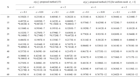
h and h2, respectively. For ex: in Table 2, let us con-sider the case 1, 0.01, N = 30 and N = 60, i.e.
1
1 30
h h (say) and 1 2
60
h h (say) and the corre-
Table 1. The maximum absolute errors for Example 4.1.
3
k
O h -proposed method (20) 2
k
O h -proposed method (31)
1
2 1 2
N
0.1
0.01 0.1 0.01 0.1 0.01 0.1 0.01
20 0.2062E–4 0.3334E–4 0.2528E–4 0.2800E–3 0.1906E–3 0.4772E–3 0.2040E–3 0.2240E–2
25 0.1519E–4 0.2511E–4 5E–4 *0.10.1810E–4 0.9455E–4 6E
34E
*0.1022E–4 *0.9075E–5 *0.1289E–4 *0.1618E
4 0.8811E–5 0.1199E–4 0.1116E
0.8989E–5 0.7612E–5 0.9217E–5 0.7880E 23E
0.887 45E
29E
88E 112E–3 0.1384E–4 E
28E
24E
7E 78E–4
28E–5 0.981 E–4 0.1
888E
64E–5 0.9179E–4 0.1148E–4 0.9831E–4 0.1143E–4
*0.1416E–4 *0.240 723E–4 *0.937 –4 0.1665E–3 0.1209E–3 0.1783E–3 0.8935E–3
–4 0.1507E–3 0.2864E–4 0.1614E–3 0.3438E–3
–4
–4 0.1402E–3 0.2224E–4 0.1502E–3 0.8741E–4
–4 0.1299E–3 0.1599E–4 0.1391E–3 0.5240E–4
45 *0.8910E–5 *0.7588E–5 *0.9148E–5 *0.78 –5 –5 0.1238E–3 0.1522E–4 0.1322E–3 0.3338E–4
50 0.8599E–5 0.6423E–5 5E–5 0.63 –5 0.1161E–3 0.1451E–4 0.1243E–3 0.1448E–4
55 *0.8066E–5 0.8110E–5 *0.5612E–5 0.5666E–5 *0.8366E–50.8420E–5 *0.440.45
60 0.7501E–5 0.4892E–5 0.7977E–5 0.28
65 *0.7070E–5 0.7123E–5 *0.4024E–5 0.4088E–5 *0.7316E–50.7362E–5 *0.2480.25
70 0.6699E–5 0.3236E–5 0.6886E–5 0.22
75 *0.6084E–5 0.6128E–5 *0.2392E–5 0.2422E–5 *0.6304E–50.6332E–5 *0.10.1907E
80 0.5511E–5 0.1772E–5 0.5834E–5 0.16
30 0.1149E–4 0.1216E–4 0.1491E–4 0.42
35 0.1082E–4 0.9128E–5 0.1348E–4 0.1661E
40 0.1030E–
–5
–5 0.1 0.1188E–3 0.1360 –4
–5 0.1059E–3 0.1325E–4 0.1135E–3 0.1284E–4
–5
–5 0.1022E–3 0.12 0.1092E–3 0.1252E–4
2E–4 0.1227 051E–3 0.1216E–4
–5
–5 0.9512E–4 0.1190E–4 0.9926E–4 0.1182E–4
*: Results obtained by using the method discussed in [13].
m absolute errors for Example 4.2
Table 2. The maximu .
3
k
h
-O 2
k
O h
-proposed method (15) proposed method (15) [for uniform mesh k1] 1
2 1 2
N
0.1
0.01 0.1 0.01 0.1 0.01 0.1 0.01
10 0.3582E–5 0.2318E–6 0.4054E–5 0.2022E–6 0.3318E–6 0.2421E–7 0.3844E–6 0.2100E–7
15 *0.4818E–6 0.4972E–6 *0.8872E–7 0.8959E–7 *0.1366E–60.1422E–6 *0.8801E–7 0.8889E–7 0.5756E–7 0.6250E–8 0.7224E–7 0.8181E–8
20 0.1104E–6 0.5934E–7 0.1951E–6 0.3283E–7 0.1929E–7 0.1412E–8 0.1616E–7 0.1012E–8
25 *0.1488E–7 0.1525E–7 *0.2740E–70.2785E–7 *0.5720E–70.5790E–7 *0.6472E–8 0.6503E–8 0.7782E–8 0.9215E–9 0.8269E–8 0.5440E–9
30 0.4865E–8 0.1987E–8 0.1354E–7 0.2173E–8 0.3116E–8 0.3812E–9 0.3880E–8 0.4004E–9
35 *0.4096E–8 0.4133E–8 *0.4312E–90.4344E–9 *0.8176E–80.8218E–8 *0.7414E–9 0.7437E–9 0.8868E–9 0.5381E–10 0.1614E–8 0.7818E–10
40 0.3373E–8 0.5659E–10 0.6534E–8 0.2147E–9 0.8617E–9 0.5733E–11 0.9210E–9 0.1817E–10
45 *0.3001E–8 0.3008E–8 *0.4228E–100.4234E–10 *0.6122E–80.6166E–8 *0.8845E–100.8872E–10 0.5417E–9 0.3230E–11 0.7106E–9 0.7117E–11
50 0.2743E–8 0.2606E–10 0.5657E–8 0.5971E–10 0.4413E–9 0.1006E–11 0.4818E–9 0.4343E–11
55 *0.2170E–8 0.2174E–8 *0.1911E–100.1918E–10 *0.4810E–80.4828E–8 *0.4804E–100.4815E–10 0.2830E–9 0.8716E–12 0.3636E–9 0.1156E–11
60 0.1676E–8 0.1210E–10 0.4138E–8 0.4104E–10 0.1978E–9 0.7677E–12 0.2442E–9 0.8821E–12
*: Results obtained by ethod 13]
[image:8.595.57.538.443.708.2]1251
order co of n ed
n other cases, e found that the order of the convergence of the method for uniform mesh case is nearly e
6. Acknowledgements
The authors thank the anonymous reviewers fo r constructive suggestions, which greatly improved the stand f the
This researc por he ty
Delhi der r nt 01
423.
7. R
rence
[1] . Kelle al Tw oun
e P lai n,
[2] P. J. Davi bi th ri
tion, ion Pr Yor
1970.
[3] . Phil I h
for Solving In
puter J l. 1 0, .
.3.2
of the nvergence method ca be estimat as 3.97 which is nearly equal to 4.0. Similarly i
w
qual to four.
r thei ard o paper.
h was sup ted by “T Universi of ” un esearch gra No. Dean (R)/R & D/2 1/
efe
s
H. B r, “Numeric Methods for o Point B d-ary Valu roblems”, B sdell, Londo 1968.
s and P. Ra nowitz, “Me od of Nume cal Integra ” 2nd Edit , Academic ess, New k,
G. M lips, “Analysis of Numerical terative Met ods tegral and In
ournal, Vo
tegro-Differential Eq 3, No. 3, 197
uations,” pp. 297-300
Com
doi:10.1093/comjnl/13 97
[4] P. Linz, “A r S in
ro-Dif qua N
44. Method fo Approximate olution of L ear Integ ferential E tions,” SIAM Journal on u-merical Analysis, Vol. 11, No. 1, 1974, pp. 137-1 doi:10.1137/0711014
[5] V. Lakshmikantham and M. R. M. Rao, “Theory of Inte-gro-Differential Equations,” Gordon and Breach, London, 1995.
[6] K. E. Atkinson, “The Numerical Solution of Integral Equations of the Second Kind,” Cambridge University Press, Cambridge, 1997.
doi:10.1017/CBO9780511626340
M App nic eer ,
1984, pp. 273-286. doi:10.1016/0045-7825(84)90009-4
[7] R. P. Agarwal and D. O’Regan, “Integral and Integro- Differential Equations: Theory, Method and Applica-tions,” Gordon and Breach, London, 2000.
[8] M. K. Jain, S. R. K. Iyenger and G. S. Subramanyam, “Variable Mesh Methods for the Numerical Solution of Two Point Singular Perturbation Problems,” Computer
ethods in lied Mecha s and Engin ing, Vol. 42
[9] R. K. Mohanty, “A Family of Variable Mesh Methods for dr) and the Solution of Nonlinear s with Singularity,”
Journal atics ol.
182, No. 1, 2005, pp. 173-187.
doi:10.1016/j.cam.2004.11.045
the Estimates of (du/
Two Point Boundary Value Problem
of Computational and Applied Mathem ,V
[10] R. K. Mohanty and N. Khosla, “A Third Order Accurate Variable Mesh TAGE Iterative M the Num
S T No gul y
Va em
Mathematics, V 26
doi:10.1080/002
ethod for
nlinear Sin ar Boundarerical olution of wo Point
lue Probl s,” International Journal o
ol. 82, No. 10, 2005, pp. 1 1-1273. f Computer
07160500113504
[11] R. K. Mohanty and N. Khosla, “Application of TAGE
I Effi Or
-tic Average Variable Mesh Discretization for Two Point
N Bo ue Ap
-matics and Computations, Vol. 172, No. 1, 2006, pp.
1 :1 .2
terative Algorithms to an cient Third der Arithme
on-Linear undary Val Problems,” plied Mathe
48-162. doi 0.1016/j.amc 005.01.134
[12] R nt of Non-Uniform e
P et is or
. K. Moha oint Arithm
y, “A Class ic Average D
Mesh Thre cretization f
( , ,
y f x y y) and the es d Mathematics and Computations , No.
p doi:10.1016/j.am 71
timates of , Vol. 183
y ,” Applie
1, 2006, p. 477-485. c.2006.05.0
[13] R. K
V sh cat E
Iterative Method y
Value Problem ge tio al
Form,” Applied Mathematics and Computations, Vol. 215,
. Mohanty and ariable Me
D. Dhal Discretization
l, “Third Order and Appli
Accurate ion of TAG for the Non-Lin
s with Homo
ear Two-Point B neous Func
oundar ns in Integr
2009, pp. 2024-2034. doi:10.1016/j.amc.2009.07.046
[14] G. Evans, “Practical Numerical Integration,” John Wiley & Sons, New York, 1993.
[15] R. S. Varga, “Matrix Iterative Analysis,” Springer-Verlag, Berlin, 2000. doi:10.1007/978-3-642-05156-2
[16] D. M. Young, “Iterative Solution of Large Linear Sys-tems,” Dover Publication, New York, 2003.
or Solving Nonlinear blems,” International
[17] C. T. Kelly, “Iterative Methods for Linear and Non-linear equations,” SIAM Publication, Philadelphia, 1995. [18] D. J. Evans, “Iterative Methods f
Two Point Boundary Value Pro