Numerical study of the linear and nonlinear dynamics near l1 and l2 points in the earth moon system

(1)

NUMERICAL STUDY OF THE LINEAR AND NONLINEAR

Department of Engineering Sciences, “Aleksand

ARTICLE INFO ABSTRACT

Studies of the restricted three

interactions in the solar system. The Lagrangian points have important applications in astronautics, since they are equilibrium points of the equation of moti

satellite or a space station. Zero velocity curves were plotted for constant values of were used to define areas of the Lagrange points of the Circular Restricted Three equations of mo

eigenvalues to investigate the stability. The invariant manifold structures of the collinear libration points for the spatial restricted three

dynamical phenomena from a geometric point of view. Earth, Moon and Earth

numerically integrated.

INTRODUCTION

The simplicity and elusiveness of the three-body problem in its various forms have attracted the attention of mathematicians for centuries. Among the giants of mathematics who have tackled the problem and made important contributions are Euler, Lagrange, Laplace, Jacobi, Le Verrier, Hamilton, Poincaré, and Birkhoff. Today the

three-enigmatic as ever and although much has been discovered already, the recent developments in nonlinear dynamics and the spur of new observations in the solar system have meant a resurgence of interest in the problem and the derivation of new results. If two bodies in the problem move in circular, coplanar orbits about their common centre of mass and the mass of the third body is too small to affect the motion of the other two bodies, the problem of the motion of the third body is called the Circular Restricted Three-Body Problem. At first glance this problem may seem to have little application to motion in the solar system. After all, the observed orbits of solar system objects are noncoplanar and noncircular. Euler and Lagrange were both awarded the Prix de l’Académie Royale des Sciences

*Corresponding author: Azem Hysa,

Department of Engineering Sciences, “Aleksand University, Durrës, Albania

ISSN: 0975-833X

Article History:

Received 04th_{October, 2015} Received in revised form

05th_{November, 2015}

Accepted 29th_{December, 2015}

Published online 31st January,2016

Citation: Azem Hysa, 2016. “Numerical study of the linear and nonlinear dynamics near Current Research, 8, (01), 25289-25294.

Key words:

Collinear libration points, Zero velocity curve, Periodic orbit.

RESEARCH ARTICLE

LINEAR AND NONLINEAR DYNAMICS NEAR

THE EARTH-MOON SYSTEM

*Azem Hysa

of Engineering Sciences, “Aleksandër Moisiu” University, Durrës, Albania

ABSTRACT

Studies of the restricted three-body problem can help in understanding the dynamics of three interactions in the solar system. The Lagrangian points have important applications in astronautics, since they are equilibrium points of the equation of motion and very good candidates to locate a satellite or a space station. Zero velocity curves were plotted for constant values of

were used to define areas of the Lagrange points of the Circular Restricted Three equations of motion were linearized to find the eigenvectors and eigenvalues.

eigenvalues to investigate the stability. The invariant manifold structures of the collinear libration points for the spatial restricted three-body problem provide the framewor

dynamical phenomena from a geometric point of view. In order to generate a trajectory around the Earth, Moon and Earth-Moon system, the two-dimensional nonlinear equations of motion were numerically integrated.

is an open access article distributed under the Creative Commons Attribution License, which distribution, and reproduction in any medium, provided the original work is properly cited.

body problem in its various forms have attracted the attention of mathematicians for centuries. Among the giants of mathematics who have tackled the problem and made important contributions are Verrier, Hamilton, -body problem is enigmatic as ever and although much has been discovered already, the recent developments in nonlinear dynamics and the spur of new observations in the solar system have meant a rgence of interest in the problem and the derivation of new If two bodies in the problem move in circular, coplanar orbits about their common centre of mass and the mass of the third body is too small to affect the motion of the other two the problem of the motion of the third body is called the . At first glance this problem may seem to have little application to motion in the solar system. After all, the observed orbits of solar system coplanar and noncircular. Euler and Lagrange were both awarded the Prix de l’Académie Royale des Sciences

Department of Engineering Sciences, “Aleksandër Moisiu”

de Paris in 1772 for their work on the three

Euler was the discoverer of the collinear equilibrium points, now known as L1, L2 and L3 (

Lagrange had a more general approach, revealing also the triangular (equilateral) equilibrium points

1873). At these points the gravitational pulls are in balance. Any infinitesimal body at any point of the Lagrangian points would be held there without getting pulled closer to either of massive bodies. Interest in the dynamics around t

points has been increasing in the last decades, as

the Sun-Earth and Earth-Moon systems have been selected for a wide variety of spatial missions (

Breakwell et al., 1974; Gómez

Masdement 2005). In 2010, the two ARTEMIS spacecraft

became the first man-made vehicles to exploit trajectories in the vicinity of an Earth-Moon libration point, operating successfully in this dynamical regime from August 2010 through July 2011, libration point

part of “The Global Exploration Roadmap” released by NASA and, as recently as June 2012, NASA has identified the collinear L1 and L2 libration points in the Earth

potential locations of interest for future human spa operations. Within the context of manned spaceflight activities, orbits near the Earth-Moon L1

lunar surface operations and serve as staging areas for future missions to near-Earth asteroids and Mars.

International Journal of Current Research

Vol. 8, Issue, 01, pp.25289-25294, January, 2016

INTERNATIONAL

Numerical study of the linear and nonlinear dynamics near L1 and L2 in the earth-moon system”,

DYNAMICS NEAR L

1

AND L

2

POINTS IN

ër Moisiu” University, Durrës, Albania

body problem can help in understanding the dynamics of three-body interactions in the solar system. The Lagrangian points have important applications in astronautics, on and very good candidates to locate a satellite or a space station. Zero velocity curves were plotted for constant values of C. The curves were used to define areas of the Lagrange points of the Circular Restricted Three-Body Problem. The tion were linearized to find the eigenvectors and eigenvalues. We computing the eigenvalues to investigate the stability. The invariant manifold structures of the collinear libration body problem provide the framework for understanding complex In order to generate a trajectory around the dimensional nonlinear equations of motion were

ribution License, which permits unrestricted use,

r work on the three-body problem. Euler was the discoverer of the collinear equilibrium points,

(Euler 1763, 1764, 1765), while

Lagrange had a more general approach, revealing also the triangular (equilateral) equilibrium points L4 and L5 (Lagrange ). At these points the gravitational pulls are in balance. Any infinitesimal body at any point of the Lagrangian points would be held there without getting pulled closer to either of massive bodies. Interest in the dynamics around the Lagrangian points has been increasing in the last decades, as L1 and L2 of Moon systems have been selected for a wide variety of spatial missions (see Farquhar 1972; 1974; Gómez et al., 1991; Canalias and

). In 2010, the two ARTEMIS spacecraft made vehicles to exploit trajectories in Moon libration point, operating successfully in this dynamical regime from August 2010 through July 2011, libration point missions were included as part of “The Global Exploration Roadmap” released by NASA and, as recently as June 2012, NASA has identified the libration points in the Earth-Moon system as potential locations of interest for future human space operations. Within the context of manned spaceflight activities, 1 and/or L2 points could support lunar surface operations and serve as staging areas for future

Earth asteroids and Mars.

INTERNATIONAL JOURNAL OF CURRENT RESEARCH

(2)

EQUATIONS OF MOTION AND METHODOLOGY

We consider the motion of the three bodies with masses and under the action of mutual gravity in three-dimensional Euclidean space. The mass of the third body-typically an asteroid, a comet, a spacecraft, or just a particle-is assumed to be negligible. The restricted three body problem is a model of the motion of the third body, affected by the gravitational attraction of two massive bodies (primaries), which describe circular orbits around their common center of masses. In order to further simplifty the problem, nondimensional quantities are used to calculate the path of the third body. The system is nondimensionalized using the following characteristic quantities: total mass, = + ; the distance between the primaries = + ; and, characteristic time, ∗= / . The nondimensional distances to the primaries are = and

= (1 − ), where = / is the ratio between the mass of one primary and the total mass of the system. So the distance between and is normalized to one. The two main bodies have a total mass that is normalized to one. Their masses are denoted by = (1 − ) and = , respectively.

The gravitational constant has been normalized to one, and the unit of time is defined such that the period of the motion of the primaries is 2 . Choose a rotating coordinate system so that the origin is at the centre of mass and and are fixed on the x-axis at (− , 0,0) and (1 − , 0,0), respectively. Let

( , , ) be the position of the third body in the rotating frame. When the movement of the third body is only studied in the plane of motion of the primaries ( = 0), the problem becomes circular planar restricted three body problem (PCRTBP). There are several ways to derive the equations of motion for this system. An efficient technique is to use the covariance of the Lagrangian formulation. This method gives the equations in Lagrangian form.

The motion ( ( ), ( ), ( )) of the third body relative to the co-rotating is described by the second order differential equations:

̈ = 2 ̇ + = 2 ̇ +

̈ = −2 ̇ − = −2 ̇ −

̈ = =

… … … … . . (1)

where is the effective potential function,

=1

2( + ) + 1 −

+ … … … (2)

and , , are the partial derivatives of with respect to the variables , , , respectively and

= ( + ) + +

and = ( + − 1) + + ,

are the distances from the third body to the primaries respectively. Equation (1) is a set of three second-order, nonlinear, coupled ordinary differential equations that are a mathematical representation of the CRTBP.

LAGRANGE POINTS AND ZERO VELOCITY CURVE

The Lagrange points L1, L2, L3, L4, and L5 of the CRTBP are the equilibrium solutions of (1). This Lagrange points are stationary only in the rotating frame and are critical points of the function (effective potential). The first Lagrange points, L1, L2, and L3, all lie on the -axis. Consider equilibria along the line of primaries where = = 0. In this case the effective potential function has the form

( , 0, 0) = −1

2 −

(1 − )

| + |−| + − 1|

It can be determined that ( , 0, 0) has precisely one critical point in each of the following three intervals along the x-axis: (i) (−∞, − ), (ii) (− , 1 − ) and (iii) (1 − ,∞). This is because ( , 0, 0) → −∞ as → ±∞, as → − , or as

→ 1 − . So

= −(1 − )( + )

| + | −

( + − 1)

| + − 1| = 0 … … … (3)

This has one solution in each of the following three intervals along the -axis. These solutions can be calculated numerically as they are the roots of polynomials. If ≠ 0 and = 0, it follows that = = 1 and so there are two Lagrangian points, denoted L4, and L5, located at the third vertex of the two equilateral triangles with the two primary masses as vertices.

The exact coordinates are: = ( , , ) = − ,√ , 0 and

= ( , , ) = − ,√ , 0 .

The system (1) has a first integral called the Jacobi integral, which is given by:

( , , , ̇, ̇, ̇) = 2 − ( ̇ + ̇ + ̇ ).

The usefulness of the Jacobi constant can be appreciated by considering the locations where the velocity of the third body is zero. In this case we have

( , , ) = 2 ( , , ) … … … (4)

(3)

Hill’s region ( , ) = {( , , )| ( , , ) ≥ /2}. The boundary of ( , ) is the zero velocity surface. The intersection of this surface with the ( , ) − plane is the zero velocity curve. The third body can move only within this region.

[image:3.595.51.270.283.348.2]

For the Earth-Moon system, = 0.01215 is know and we can solve the equation (3) numerically in Matlab and we find the location of the Lagrangian points (L1, L2, and L3). The locations of the equilateral triangle libration points are much easier to compute. The value of the Jacobi integral at point ( = 1,2,3,4,5) will be denoted by . The non-dimensional rotating frame coordinates ( , , ) of each of the five libration points for the Earth-Moon system value of appear in Table 1 along with the value associated with a stationary located at each point of equilibrium.

Table 1. Earth-Moon libration point rotating frame locations and “energy” values

0.8369 0 0 3.1883

1.1557 0 0 3.1722

-1.0051 0 0 3.0121

0.48785 +0.866 0 2.9880

[image:3.595.39.277.414.645.2]

0.48785 - 0.866 0 2.9880

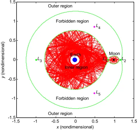
Figure 1 shows the location of the libration points and the zero velocity curve at the energy level of for the Earth-Moon system. In this figure, there are three mains realms; namely the inner region, outer region and the forbidden region.

Fig. 1. The five libration points and the zero velocity curve at for the Earth-Moon system

The plot suggests that the barrier between the Earth and the Moon is just opening at the energy . This is the reason for the name . It is the first point where the Jacobi surface begins to “tear”. The barrier between the Earth and the Moon has now reseeded, and there is a “neck” near through which a trajectory might pass. In fact the linearized dynamics at show it to be a fixed point of “center×saddle” type, and while

most orbits will be ejected from this neck region, the presence of the center manifold in the nonlinear problem suggests that we may be able to find periodic orbits in the neck, which orbit

or .

LINEARIZATION OF THE CRTBP AT THE

LAGRANGE POINTS

Because the Circular Restricted Three-Body Problem is non-linear dynamics, there is no general, easy analytical solution. But, some particular solutions such as linearization or perturbation method can give restricted analytical solution, and some numerical methods, such as differential corrector and Poincare map, can also useful for finding advantageous trajectory and periodic orbits. Because the CRTBP has no analytical solution, it is necessary to numerically equations of motion in order to propagate a three-body orbit. This first requires that the equations be formulated as a system of ODEs. We introduce the state vector x and its time derivative ̇. These are six-element column vectors, containing the position and velocity and the velocity and acceleration, respectively.

̇ = =

⎝ ⎜ ⎜ ⎛

̇

2 ̇ + −2 ̇ +

⎠ ⎟ ⎟ ⎞

= … … … … . . (5)

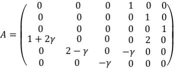
Analysis of orbit stability also requires numerical methods. We begin by defining the A matrix, which is the Jacobian of the state derivative ̇. This matrix is defined generally as:

= ̇ … … … . (6)

In addition to describe the instantaneous dynamics of orbit, the matrix is used to define the state transition matrix, Φ( , ). This matrix maps deviations from the initial state forward to time t. It is defined by the differential equation: Φ̇ ( , ) =

Φ( , ) with the initial condition Φ = . The state transition matrix must be integrated along with the state. This most easily done by creating one long state vector, = [ ,Φ] , where the elements of Φ have been reshaped into a 36 × 1 column vector. A special case of the state transition matrix is the monodromy matrix, . This is defined as the matrix mapping initial deviations forward by one orbital period: =Φ( , ). The monodromy matrix is important because it contains information about the stability along the entire orbit. In the CRTBP, the matrix is greatly simplified, as most of the derivatives are zero. After deriving expressions for each of the derivatives, we get a matrix of the following form:

=

⎝ ⎜ ⎜ ⎛

0 0 0 0 0 0 0 0 0

1 0 0 0 1 0 0 0 1 1 + 2 0 0

0 2 − 0

0 0 −

0 2 0

− 0 0

0 0 0⎠ ⎟ ⎟ ⎞

… … … . (7)

where = (1 − )/| + | + /| + − 1| .

-1.5 -1 -0.5 0 0.5 1 1.5

x (nondimensional)

y

(

n

o

n

d

im

e

n

s

io

n

a

l)

L₁ L₂ L₃

L

4

L₅

Earth Moon

Forbidden region

[image:3.595.306.483.657.726.2]

(4)

RESULTS AND CONCLUSIONS

Using for the Earth-Moon system and plugging the coordinates for into the system matrix gives a constant, whose eigenvalues and eigenvectors are

= +2.9316 = −2.9316 = +2.3341

= − 2.3341 = +2.2686 = −2.2686 and = ⎝ ⎜ ⎜ ⎛ −0.2933 0.1350 0 −0.8598 0.3957 0 ⎠ ⎟ ⎟ ⎞ , = ⎝ ⎜ ⎜ ⎛ −0.2933 −0.1350 0 0.8598 0.3957 0 ⎠ ⎟ ⎟ ⎞ = ⎝ ⎜ ⎜ ⎛

−0.1058 − 0.0000i −0.0000 − 0.3793i

0

−0.0000 − 0.2469i 0.8854 0 ⎠ ⎟ ⎟ ⎞ = ⎝ ⎜ ⎜ ⎛

−0.1058 + 0.0000i −0.0000 + 0.3793i

0

−0.0000 + 0.2469i 0.8854 0 ⎠ ⎟ ⎟ ⎞ = ⎝ ⎜ ⎜ ⎛ 0 0 0 – 0.4034

0 0 0.9150 ⎠ ⎟ ⎟ ⎞ , = ⎝ ⎜ ⎜ ⎛ 0 0 0 + 0.4034

0 0 0.9150 ⎠ ⎟ ⎟ ⎞

respectively, which is the classical " × "

behavior we expect at . The linear analysis tells us that has a one dimensional stable direction (manifold), and one dimensional unstable direction (manifold), and a two dimensional center (manifold). Repeating this analysis at and gives

= −2.1582 = +2.1582 = +1.8624 = −1.8624 = +1.7859 = −1.7859 = ⎝ ⎜ ⎜ ⎛ 0.3556 0.2242 0 −0.7676 −0.4838 0 ⎠ ⎟ ⎟ ⎞ , = ⎝ ⎜ ⎜ ⎛ −0.3556 0.2242 0 −0.7676 0.4838 0 ⎠ ⎟ ⎟ ⎞ = ⎝ ⎜ ⎜ ⎛

−0.1536 + 0.0000i −0.0000 − 0.4474i

0

−0.0000 − 0.2861i 0.8333 0 ⎠ ⎟ ⎟ ⎞ = ⎝ ⎜ ⎜ ⎛

−0.1536 – 0.0000i −0.0000 + 0.4474i

0

−0.0000 + 0.2861i 0.8333 0 ⎠ ⎟ ⎟ ⎞ = ⎝ ⎜ ⎜ ⎛ 0 0 0 + 0.4886

0 0 −0.8725 ⎠ ⎟ ⎟ ⎞ , = ⎝ ⎜ ⎜ ⎛ 0 0 0 − 0.4886

0 0 −0.8725 ⎠ ⎟ ⎟ ⎞ and = −2.1582 = +2.1582 = +1.8624 = −1.8624 = +1.7859 = −1.7859 = ⎝ ⎜ ⎜ ⎛

−0.3146 – 0.0000 0.0000 – 0.6292

0 0.0000 – 0.3178

0.6357 0 ⎠ ⎟ ⎟ ⎞ = ⎝ ⎜ ⎜ ⎛

−0.3146 + 0.0000 0.0000 + 0.6292

0

0.0000 + 0.3178 0.6357 0 ⎠ ⎟ ⎟ ⎞ = ⎝ ⎜ ⎜ ⎛ −0.1159 −0.9778 0 0.0205 0.1732 0 ⎠ ⎟ ⎟ ⎞ , = ⎝ ⎜ ⎜ ⎛ 0.1159 −0.9778 0 0.0205 −0.1732 0 ⎠ ⎟ ⎟ ⎞ = ⎝ ⎜ ⎜ ⎛ 0 0 0 – 0.7052

0 0 0.7090 ⎠ ⎟ ⎟ ⎞ , = ⎝ ⎜ ⎜ ⎛ 0 0 0 + 0.7052

0 0 0.7090 ⎠ ⎟ ⎟ ⎞

(5)

[image:5.595.39.287.53.274.2] [image:5.595.39.288.313.534.2]

Fig. 2. Halo orbits around the point and in the Earth-Moon system

Fig. 3. Stable (cyan) and unstable (magenta) manifolds associated with and Halo orbits in the Earth-Moon system

The instability of Halo orbits and similar periodic solutions can be exploited to analyze paths to and from every point on a given orbit. While there are infinitely many of these paths, they all belong to a well-defined set called a manifold. Matlab programming was used to develop manifolds for the CRTBP. Suitable values are 1e-12 for RelTol and 1e-10 for AbsTol. The manifolds associated to the periodic orbits are centered on the manifolds of the points. These 2-dimensional subspaces are here called M , , M , , M , and M , . Figure 3 shows four manifolds in the Earth-Moon system.

The first, in cyan, is the stable manifold M , of point in the the outer region. This is set of trajectories moving forward in time that asymptotically approach the Halo orbit. In contrast, the second plot in magenta depicts the unstable manifold

M , , which departs the Halo orbit over time. The interior manifolds M , and M , are stable and unstable manifolds of Earth-Moon Lagrange point, respectively. If the third body is on a stable manifold, its trajectory winds onto the orbit and, if it is on the unstable one, it winds off the orbit. This aspect is very important for the design of missions about the libration points, for instance, in the Earth-Moon system. The stable and unstable manifolds for a symmetric orbit are themselves symmetric about the axis. This is because the two experience equal and opposite rotation rates: counter-clockwise for forward time (unstable) and clockwise for backward time (stable). In order to generate a trajectory around the Earth and Moon for the CRTBP, the two-dimensional nonlinear equations of motion were numerically integrated.

̇ = ̇ =

̇ = 2 + − (1 − )( + )+ ( + − 1)

̇ = −2 + − (1 − ) +

… … . . (8)

The state-space representation of the equations of motion (Equation 8) was programmed into Matlab. The set of four, first order, nonlinear equations were numerically integrated using the RK4 method. The value of corresponds to a body (third body) traveling around the Moon and the Earth or the Earth-Moon system. Moderately stringent tolerances are necessary to reproduce the qualitative behavior of the orbit. Suitable values are 1e-11 for RelTol and 1e-11 for AbsTol.

Fig. 4. The path of the third body around the Earth

Figures (4) and (5) show, in rotating coordinates two periodic orbits which begin near the Earth or Moon, respectively, and seem to stay in orbit around them. The initial conditions for these orbits are: (0) = 0.12, (0) = 0, (0) = 0, (0) = 3.2901 and (0) = 1.06, (0) = 0, (0) = 0, (0) = 0.4638, respectively.

0.8 0.85 0.9 0.95 1 1.05 1.1 1.15 1.2

-0.1 -0.05 0 0.05 0.1 0.15

y

(

no

n

d

im

en

s

io

n

a

l)

L

1 L2

Moon ZVC

L

1 L2

Moon ZVC

-4 -3 -2 -1 0 1 2

-3 -2 -1 0 1 2 3

L

2

L

2

Moon Moon

L

1

L

1

L

4

L

4

L

5

L

5

Earth Earth

Inner region Inner region region region Forbidden Forbidden

L

3

L

3

Outer region Outer region

y

(n

on

dim

en

sio

na

l)

-0.2 -0.1 0 0.1 0.2

-0.25 -0.2 -0.15 -0.1 -0.05 0 0.05 0.1 0.15 0.2 0.25

y

(

n

on

d

im

e

n

s

io

n

al)

[image:5.595.309.561.426.643.2]

(6)

[image:6.595.42.284.55.269.2]

Fig. 5. The path of the third body around the Moon

Fig. 6. Long integration of the transfer orbit for t=700 time units

The trajectories are very sensitive to initial conditions it is hoped that by playing with the initial data a an orbit with the desired trajectory could be found. Once an orbit is found which goes from the Earth side of to the Moons, the orbit is

integrating forward forward gives an orbit which starts near the Earth and goes around the Moon. If we integrate the system longer an even more interesting picture develops. To find the desired orbit we begin with initial conditions: (0) = 0.83,

(0) = 0, (0) = 0, (0) = 0.1444 near .

If the system is integrated this way for a long time (forward and backward) we get the pictures in Figure 6.

Acknowledgements

The author is thankful to the reviewers for their valuable suggestions to enhance the quality of my article.

REFERENCES

Amanda, H.F, Kathleen, Howell F. 2014. Representations of higher-dimensional Poincaré maps with applications to spacecraft trajectory design, Acta Astronautica, 96, 23–41. Canalias E, Delshams A, Masdemont J.J and Roldán P. 2006. The scattering map in the planar restricted three body problem, Celestial Mechanics and Dynamical Astronomy, 95:155–171 DOI 10.1007/s10569- 006-9010-4.

Dellintiz M, Ober-Blo ̈baum S, Post M, Schu ̈tze O and Thiere B. A 2009. multi-objective approach to the design of low thrust space trajectories using optimal control, PACS: 95.10.Ce, 02.60.Pn, 45.20.Jj, 45.80.+r, 45.10.Db.

Folta DC, Pavlak ThA, Haapala AF, and Howell KC. 2013. Preliminary design considerations for access and operations in earth-moon L_1/L_2 orbits, AAS 13-339.

Gidea M, Deppe F, and Anderson G, 2007. Phase space reconstruction in the restricted three-body problem, Publ. Natl. Astron. Obs. Japan, Vol. 9, 55.

Gomez G, Koon WS, Lo MW, Marsden J E, Masdemont J and SD. Ross. 2004. Connecting orbits and invariant manifolds in the spatial restricted three-body problem, Institute of Physics Publishing, Nonlinearity 17, 1571–1606, PII: S0951-7715(04)67794-2.

Murray CD and Dermott SF. 1999. Solar System Dynamics. Cambridg University press, 1st edition, 0-52157295-9 (hc.). 521-57597-4 (pbk.).

Posnitskii SP, 2008. On the stability of triangular Lagrangian points in the restricted three- body problem, The Astronomical Journal, 135:187–195.

Truesdale N. 2012. Using Invariant Manifolds of the Sun-Earth L2 Point for Asteroid Mining Operations, Spaceight Dynamics, ASEN, 5050.

0.85 0.9 0.95 1 1.05 1.1

-0.1 -0.05 0 0.05 0.1 0.15

y

(

n

o

nd

imen

s

io

na

l)

Moon

-1.5 -1 -0.5 0 0.5 1 1.5

y

(

n

o

nd

im

e

n

s

io

n

a

l)

L₁ L₂ L₃

L₄

L₅

Earth Moon

Forbidden region

Forbidden region Inner region Outer region

Outer region

[image:6.595.43.283.307.534.2]