A Nonlinear Autoregressive Scheme for Time Series Prediction via Artificial Neural Networks

(1)

ISSN Online: 2327-5227 ISSN Print: 2327-5219

DOI: 10.4236/jcc.2018.69002 Sep. 7, 2018 14 Journal of Computer and Communications

A Nonlinear Autoregressive Scheme for Time

Series Prediction via Artificial Neural Networks

Rohit Raturi

1

, Hayk Sargsyan

2

1_{Regional Development Center, KPMG USA LLP, Montvale, NJ, USA}

2_{Institute of Informatics, National Academy of Sciences of Armenia, Yerevan, Armenia}

Abstract

This article is devoted to a time series prediction scheme involving the nonli-near autoregressive algorithm and its applications. The scheme is imple-mented by means of an artificial neural network containing a hidden layer. As a training algorithm we use scaled conjugate gradient (SCG) method and the Bayesian regularization (BReg) method. The first method is applied to time series without noise, while the second one can also be applied for noisy data-sets. We apply the suggested scheme for prediction of time series arising in oil and gas pricing using 50 and 100 past values. Results of numerical simula-tions are presented and discussed.

Keywords

Nonlinear Autoregression, Time Series, Prediction, Data Analysis, Deep Learning, Scaled Conjugate Gradient Method, Bayesian Regularization Method

1. Introduction

Any branch of science which deals with observational data, requires a repeatedly usage of the mathematical concept of time series. Time series are formed by dis-crete measurements of a specific quantity at successive time instants. They are used in such disciplines as statistics [1] including statistical physics and me-chanics; astronomy including astrophysics, celestial mechanics and cosmology

[2]; oceanography [3]; econometrics and mathematical finance including actu-arial mathematics [4] [5]; meteorology and climatology [6]; seismology [7]; bi-ology [8]; engineering [9]; earth science and geomechanics [10], etc. Examples of time series include (in an order corresponding to the disciplines above) positions of particles under Brownian motion; tidal heights; assets of a company; speed How to cite this paper: Raturi, R. and

Sargsyan, H. (2018) A Nonlinear Autore-gressive Scheme for Time Series Prediction via Artificial Neural Networks. Journal of Computer and Communications, 6, 14-23. https://doi.org/10.4236/jcc.2018.69002

Received: July 24, 2018 Accepted: September 4, 2018 Published: September 7, 2018

(2)

DOI: 10.4236/jcc.2018.69002 15 Journal of Computer and Communications

and direction of a weather flow; seismic activity; population of species; load-deformation dependence of structures; displacement of the crust of the Earth.

The mathematical analysis of time series is a very important branch of statis-tics. A proper mathematical analysis may reveal the most important features of the temporal measurements and use the output to make a meaningful insight. The most desirable insight might be a prediction of future behavior of a pheno-mena/process based on the past data. We learn that from the ancient time hu-mans were able to do astronomical, meteorological, seismic, etc. predictions. For example, based on the seismic activity of a specific region, many centuries ago people on different continents were able to predict a time frame when the high-est-risk seismic behavior will occur in that region and thus had an opportunity for safe evacuation. Another example, the analysis of astronomical data gathered by known astronomers such as Tycho Brahe, Johann Kepler was able to for-mulate his law, which was laid in the foundations of celestial mechanics much later.

All this and much more are now easily performed based on the fundamental methods of contemporary statistical analysis. One of the most powerful methods allowing analyzing time series and make predictions, is the nonlinear au-to-regression algorithm (NAR). For a detailed introduction into the subject, see

[11] [12] and the related references therein. The algorithm was developed to analyze periodically sampled data [13] [14] (more often equally or regularly spaced term is used). However, recently the algorithm has been extended to be applicable for analyzing equally or regularly spaced data [15]. The algorithm and its modifications are used by several authors to train artificial neural networks for predictive analysis of time series with many applications [16] [17].

In this article we apply the nonlinear autoregressive model for a predictive analysis of time series arising in gas and oil pricing. The data used in this paper are freely available at the Macrotrends webpage1_{. The paper is organized as} fol-lows. We first briefly describe the nonlinear autoregressive model we use in Sec-tion 2. In SecSec-tion 3 we present the results of numerical simulaSec-tions performed in MatLab. In particular, among others, it is established how the performance of the algorithm for a specific time series depends on the number of data used for forecasting future values of the series.

2. Nonlinear Autoregressive Model: Main Relations and

Characteristics

The nonlinear autoregressive model is defined for an order p∈. Thus, the nonlinear autoregressive model of order p is defined as [17]

( )

(

1 ,

) (

2 , ,

)

(

)

( )

,

f t =F f t− f t−  f t p− +ε t

where f t

( )

is the current value and, apparently, f t i i

(

−

)

, =1,2, ,_ p is the

(3)

dependence of the current value on the past p values of the time series,

ε

_{is a}

white noise. This means that every current value depends on the previous p

values.

The main aim of any method of statistical analysis is the low-error approximation of F. In the simplest case, F is a linear function, leading to

( )

0

(

) ( )

1 ,

p i i

f t F F f t i ε t

=

= +

∑

− +

where F0 and F ii, 1,2, ,=  p are given constants.

Structure of the Nonlinear Autoregressive Model Based Artificial

Neural Network

The nonlinear autoregressive model based neural network, is a feed-forward network aiming to approximate F in the above definition. The feed-forward algorithm is defined by [17]

( )

(

) (

)

(

)

ˆ ˆ _{1 ,} _{2 , ,} _,

f t =F f t− f t−  f t p− (1)

( )

0

( )

1 1

ˆ N _i _k p _ik _,

i k

f t α αA β w f t

= =

 

= + _ + _

 

∑

(2)

where α =i, 1,2, ,i  N are constants, A is the activation function, wik are the weights, βk are the biases.

NAR methods are efficiently used for forecasting as deterministic models, as well as stochastic models. In this study, we consider a three-layer neural network, in which the feed-forward algorithm (1), (2) is learned using the well-known supervised learning algorithm scaled conjugate method developed in [18], as well as the Bayesian regularization presented in [19] in details.

3. Application of the Nonlinear Autoregressive Model for

Prediction of Gas and Oil Prices

Let us proceed with the implementation of the algorithm described in the previous two sections. For simplicity, let the time series of past values be composed of 50 data. This means that the nonlinear autoregressive model of order p = 50 must be involved. To measure the error between the target and output, we use the mean square error function

(

)

(

)

2

1

Er ,i i N i i , i

o t o t

=

∑

−

with oi being the outputs and ti being the targets. We also compute the correlation coefficient to compare the statistical properties of the analysis for different order NAR models:

(

)

( )

1

(

)

(

)

1 _.

Er , Er ,

N

i i i

i i

C o o t t

o o t t =

= − −

⋅

∑

(4)

[image:4.595.214.535.273.463.2] [image:4.595.211.540.490.687.2]

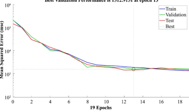
Figure 1. At this, the best performance occurs at 13th_{iteration and is equal to} 1512.9115. The gradient and validation check results are plotted in Figure 2. It is evident that the gradient is a locally decreasing function of epochs, which means that if more iterations are involved, the error should be decreased. On the other hand, we see that the validation checks increase when the number of epochs increases.

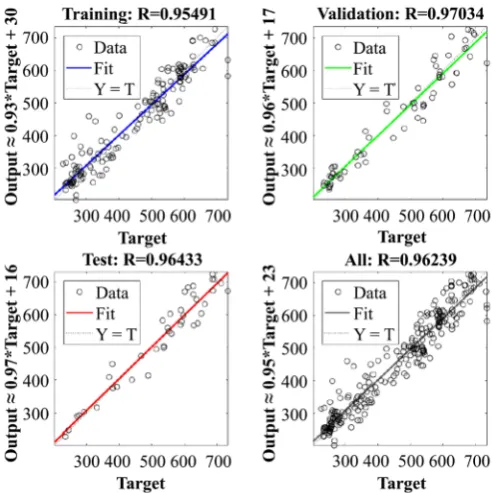
From Figure 3, where the error histogram is plotted, it is easy to observe that near the zero error (i.e., when the target and output are equal) the training errors for positive difference is comparably higher than for negative difference. It is also noteworthy that the training regression plot shows a high efficiency of the fitting tool of the algorithm (see Figure 4).

Finally, let us summarize the main result of the numerical simulation. As it is

Figure 1. Performance of the neural network: p = 50.

Figure 2. The training state, i.e., gradient and validation checks against iteration number:

(5)

[image:5.595.217.532.73.248.2]

Figure 3. Error histrogram: the dependence of the target and output difference on time instances: p = 50.

Figure 4. Training regression: p = 50.

[image:5.595.249.496.294.541.2]

(6)

[image:6.595.208.540.78.253.2] [image:6.595.210.540.292.481.2]

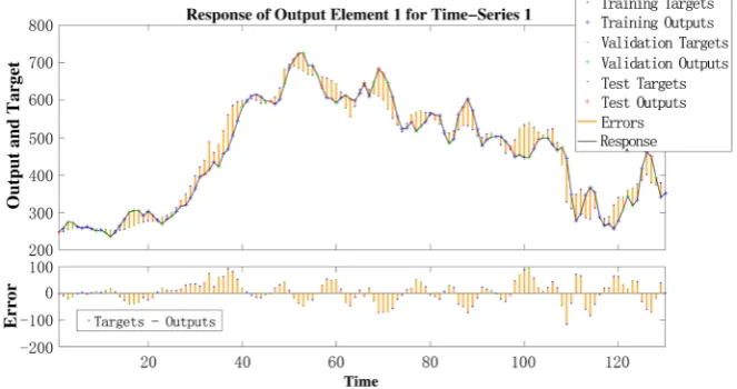
[image:6.595.211.534.510.703.2]

Figure 5. Output element response for the time series: p = 50.

Figure 6. Autocorrelation of error: p = 50.

(7)

[image:7.595.230.518.73.242.2]

Figure 8. The training state, i.e., gradient and validation checks against iteration number:

[image:7.595.229.516.290.451.2]

p = 100.

Figure 9. Error histrogram: the dependence of the target and output difference on time instances: p = 100.

[image:7.595.276.473.500.708.2]

(8)

[image:8.595.219.529.72.251.2]

Figure 11. Output element response for the time series: p = 100.

Figure 12. Autocorrelation of error: p = 100.

4. Conclusion

In this article we show the efficiency of the nonlinear autoregression algorithm based artificial neural network in time series analysis and prediction. As a particular model we choose the time series generated by daily prices of gas and oil (the data are freely available at www.mactrotrends.com). The artificial neural network consists of 3 layers: an input layer, a hidden layer, an output layer. Using the scaled conjugate gradient method to learn the neurons, we test the algorithm for 50 and 100 number of past values. The main characteristics of the neural network performance are reported. In particular, a significant improve is observed in validation and regression, the gradient is decreased, the target/output error is decreased almost two time and autocorrelation error is decreased almost 2.5 times.

Acknowledgements

[image:8.595.227.521.287.462.2]

(9)

that helped to improve the presentation of the material.

Conflicts of Interest

The authors declare no conflicts of interest regarding the publication of this pa-per.

References

[1] Anderson, T.W. (1994) The Statistical Analysis of Time Series. Wiley-Interscience, Hoboken, NJ.

[2] Maoz, D., Sternberg, A. and Leibowitz, E.M. (1997) Astronomical Time Series. Kluwer Academic Publishers, Help: IPA for Dutch.

[3] Emery, W.J. and Thomson, R.E. (2014) Data Analysis Methods in Physical Oceano-graphy. 3rd Edition, Elsevier, Amsterdam, Netherlands.

[4] Zivot, E. and Wang, J.H. (2002) Modeling Financial Time Series with S-PLUS. Springer-Verlag, Berlin.

[5] Diebold, F.X. (2017) Time-Series Econometrics: A Concise Course. University of Pennsylvania, Pennsylvania.

[6] Duchon, C. and Hale, R. (2011) Time Series Analysis in Meteorology and Clima-tology: An Introduction. Wiley-Blackwell, Hoboken, NJ.

[7] Chelidze, T., Vallianatos, F. and Telesca, L. (2018) Complexity of Seismic Time Se-ries: Measurement and Application. Elsevier, Amsterdam, Netherlands.

[8] Tapinos, A. (2012) Time Series Data Mining In Systems Biology. A Thesis Submit-ted for the Degree of Doctor of Philosophy, The University of Manchester, Man-chester.

[9] Abdelhamid, T.S. and Everett, J.G. (1999) Time Series Analysis for Construction Productivity Experiments. Journal of Construction Engineering and Management, 125, 87-95. https://doi.org/10.1061/(ASCE)0733-9364(1999)125:2(87)

[10] Trauth, M. (2015) MATLAB Recipes for Earth Sciences. 4th Edition, Springer, Ber-lin. https://doi.org/10.1007/978-3-662-46244-7

[11] Lu, S. and Chon, K.H. (2003) Nonlinear Autoregressive and Nonlinear Autoregres-sive Moving Average Model Parameter Estimation by Minimizing Hypersurface Distance. IEEE Transactions on Signal Processing, 51, 3020-3026.

[12] Brockwell, P.J., Dahlhaus, R. and Trindade, A.A. (2005) Modified Burg Algorithms for Multivariate Subset Autoregression. Statistica Sinica, 15, 197-213.

[13] Udny, Y.G. (1927) On a Method of Investigating Periodicities in Disturbed Series, with Special Reference to Wolfer’s Sunspot Numbers. Philosophical Transactions of the Royal Society A, 226, 636-646. https://doi.org/10.1098/rsta.1927.0007

[14] Walker, G. (1931) On Periodicity in Series of Related Terms. Proceedings of the Royal Society A, 131, 518-532. https://doi.org/10.1098/rspa.1931.0069

[15] Bos, R., De Waele, S. and Broersen, P.M.T. (2002) Autoregressive Spectral Estima-tion by ApplicaEstima-tion of the Burg Algorithm to Irregularly Sampled Data. IEEE Transactions on Instrumentation and Measurement, 51, 1289-1294.

https://doi.org/10.1109/TIM.2002.808031

[16] Potdar, K. and Kinnerkar, R. (2017) A Non-Linear Autoregressive Neural Network Model for Forecasting Indian Index of Industrial Production. IEEE Region 10

Symposium (TENSYMP), Cochin, India, 14-16 July 2017.

(10)

[17] Tealab, A., Hefny, H. and Badr, A. (2017) Forecasting of Nonlinear Time Series Using ANN. Future Computing and Informatics Journal, 2, 39-47.

https://doi.org/10.1016/j.fcij.2017.05.001

[18] Moller, M.F. (1993) A Scaled Conjugate Gradient Algorithm for Fast Supervised Learning. Neural Networks, 6, 525-533.

https://doi.org/10.1016/S0893-6080(05)80056-5