University of Central Florida University of Central Florida
STARS
STARS
Electronic Theses and Dissertations, 2004-2019
2018
Towards High-Performance Big Data Processing Systems
Towards High-Performance Big Data Processing Systems
Hong ZhangUniversity of Central Florida
Part of the Computer Sciences Commons
Find similar works at: https://stars.library.ucf.edu/etd
University of Central Florida Libraries http://library.ucf.edu
This Doctoral Dissertation (Open Access) is brought to you for free and open access by STARS. It has been accepted for inclusion in Electronic Theses and Dissertations, 2004-2019 by an authorized administrator of STARS. For more information, please contact [email protected].
STARS Citation STARS Citation
Zhang, Hong, "Towards High-Performance Big Data Processing Systems" (2018). Electronic Theses and Dissertations, 2004-2019. 5966.
TOWARDS HIGH-PERFORMANCE BIG DATA PROCESSING SYSTEMS
by
HONG ZHANG
M.S. University of Wyoming, 2015
A dissertation submitted in partial fulfilment of the requirements for the degree of Doctor of Philosophy
in the Department of Computer Science in the College of Engineering and Computer Science
at the University of Central Florida Orlando, Florida
Summer Term 2018
c
ABSTRACT
The amount of generated and stored data has been growing rapidly, It is estimated that 2.5 quintil-lion bytes of data are generated every day, and 90% of the data in the world today has been created in the last two years. How to solve these big data issues has become a hot topic in both industry and academia.
Due to the complex of big data platform, we stratify it into four layers: storage layer, resource management layer, computing layer, and methodology layer. This dissertation proposes brand-new approaches to address the performance of big data platforms like Hadoop and Spark on these four layers.
We first present an improved HDFS design called SMARTH, which optimizes the storage layer. It utilizes asynchronous multi-pipeline data transfers instead of a single pipeline stop-and-wait mech-anism. SMARTH records the actual transfer speed of data blocks and sends this information to the namenode along with periodic heartbeat messages. The namenode sorts datanodes according to their past performance and tracks this information continuously. When a client initiates an upload request, the namenode will send it a list of “high performance” datanodes that it thinks will yield the highest throughput for the client. By choosing higher performance datanodes relative to each client and by taking advantage of the multi-pipeline design, our experiments show that SMARTH significantly improves the performance of data write operations compared to HDFS. Specifically, SMARTH is able to improve the throughput of data transfer by 27-245% in a heterogeneous virtual cluster on Amazon EC2.
Secondly, we propose an optimized Hadoop extension called MRapid, which significantly speeds up the execution of short jobs on the resource management layer. It is completely backward
com-cloud show that MRapid can improve performance by up to 88% compared to the original Hadoop.
Thirdly, we introduce an efficient 3-level sampling performance model, called Hedgehog, and fo-cus on the relationship between resource and performance. This design is a brand new white-box model for Spark, which is more complex and challenging than Hadoop. In our tool, we employ a Java bytecode manipulation and analysis framework called ASM [1] to reduce the profiling over-head dramatically.
Fourthly, on the computing layer, we optimize the current implementation of SGD in Spark’s MLlib by reusing data partition for multiple times within a single iteration to find better candidate weights in a more efficient way. Whether using multiple local iterations within each partition is dynamically decided by the 68-95-99.7 rule. We also design a variant of momentum algorithm to optimize step size in every iteration. This method uses a new adaptive rule that decreases the step size whenever neighboring gradients show differing directions of significance. Experiments show that our adaptive algorithm is more efficient and can be 7 times faster compared to the original MLlib’s SGD.
At last, on the application layer, we present a scalable and distributed geographic information system, called Dart, based on Hadoop and HBase. Dart provides a hybrid table schema to store spatial data in HBase so that the Reduce process can be omitted for operations like calculating the mean center and the median center. It employs reasonable pre-splitting and hash techniques to avoid data imbalance and hot region problems. It also supports massive spatial data analysis like K-Nearest Neighbors (KNN) and Geometric Median Distribution. In our experiments, we evaluate the performance of Dart by processing 160 GB Twitter data on an Amazon EC2 cluster. The experimental results show that Dart is very scalable and efficient.
ACKNOWLEDGMENTS
I would first like to express my sincere gratitude to my adviser, Professor Liqiang Wang for his patient guidance, continuous encouragement and significant support during my Ph.D study. He not only inspired me in research, but also gave me many advices on life and future career.
I would like to thank my current and former committee members, Dr. Damla Turgut, Dr. Jun Wang, Dr. Shunpu Zhang, and Dr. Boqing Gong. I am very grateful for their invaluable advice and patience with me over these days. Genuine thanks to each of them for the extraordinary amount of time and knowledge they were willing to provide on my dissertation.
I dedicate this thesis to my family: my parents Linsheng Zhang and Fenglan Zhao, as well as my wife Rui Guo, for their endless love, selfless care and support. Thanks to my lovely daughter Rosie who inspires me to keep going and brings me full of happiness every day.
I would like to thank all the former and current graduate students in Dr. Liqiang Wang’s research group. They are Zixia Liu, Siyang Lu, BingBing Rao, Hongyi Ma, He Huang, Ping Guo, Chao Liang, Zhibo Sun, Yifan Ding, Yandong Li, and Ehsan Kazemy.
Last but not least, I would like to thank all my collaborators for discussions I had with them and ideas they gave to me. They are Dr. Hai Huang, Dr. Chen Xu, Weidong Wang, Yong Yang, Lei Chen, and Xiang Wei.
TABLE OF CONTENTS
LIST OF FIGURES . . . xi
LIST OF TABLES . . . xv
CHAPTER 1: INTRODUCTION . . . 1
1.1 Storage Layer . . . 2
1.2 Resource Management Layer . . . 3
1.3 Computing Layer . . . 6
1.4 Methodology Layer . . . 8
CHAPTER 2: LITERATURE REVIEW . . . 11
2.1 HDFS System and Data Uploading . . . 12
2.2 Resource Management and Scheduling . . . 14
2.3 Performance Modeling . . . 18
2.4 Structured Big-data Store . . . 20
CHAPTER 3: ENABLING MULTI-PIPELINE DATA TRANSFER IN HDFS . . . 23
3.2 Global Optimization for Data Transmission . . . 26
3.3 Local Optimization for Data Transmission . . . 27
3.4 Cost-Benefit Analysis . . . 28
3.5 Fault Tolerance . . . 32
3.5.1 Fault Tolerance for Original HDFS . . . 32
3.5.2 Fault Tolerance for Multi-Pipelines . . . 33
3.5.3 Buffer Overflow Problem . . . 34
3.6 Experiments . . . 34
3.6.1 Two-Rack Cluster Scenario . . . 35
3.6.2 Bandwidth Contention Scenario . . . 40
3.6.3 Heterogeneous Cluster Scenario . . . 42
3.7 Conclusions . . . 43
CHAPTER 4: AN EFFICIENT SHORT JOB OPTIMIZER ON BIG-DATA PLATFORM . 45 4.1 Distributed Mode . . . 46
4.2 Improved Uber Mode . . . 51
4.3 Job Submitting Framework and Speculative Execution . . . 53
4.4.1 Experimental Results on A3 Cluster . . . 59
4.4.2 Experimental Results for A2 Cluster . . . 63
4.5 Conclusions . . . 66
CHAPTER 5: TUNING PERFORMANCE FOR BIG-DATA PLATFORM . . . 67
5.1 Hedgehog Structure . . . 67
5.2 Performance Model . . . 70
5.3 Experiments . . . 71
5.4 Conclusions . . . 71
CHAPTER 6: AN ADAPTIVE STOCHASTIC GRADIENT DESCENT ALGORITHM ON BIG-DATA PLATFORM . . . 72
6.1 Background . . . 72
6.2 Design and Implementation . . . 76
6.2.1 Parallel SGD with iterative local search . . . 78
6.2.2 68-95-99.7 Rule . . . 79
6.2.3 Parallel SGD with Adaptive Momentum . . . 80
6.3 Experiments . . . 84
6.3.2 Experiments with Adaptive Learning Rate . . . 88
6.3.3 Experiments with Different Size of Partitions . . . 92
6.4 Conclusions . . . 93
CHAPTER 7: AN EFFICIENT GEOSPATIONAL AND TEMPORAL ANALYTICS FRAME-WORK . . . 94 7.1 System Structure . . . 95 7.2 Methodology . . . 96 7.2.1 Geographic mean . . . 97 7.2.2 Geographic midpoint . . . 97 7.2.3 Geographic Median . . . 97 7.3 Data Analysis . . . 102 7.3.1 K Nearest Neighbors . . . 103 7.3.2 Spatial distribution . . . 103 7.4 Experiments . . . 104
CHAPTER 8: CONCLUSION AND FUTURE WORK . . . 112
APPENDIX A: COPYRIGHT PERMISSION INTERNATIONAL CONFERENCE ON PARALLEL PROCESSING . . . 114
APPENDIX B: COPYRIGHT PERMISSION
INTERNATIONAL PARALLEL AND DISTRIBUTED PROCESSING SYM-POSIUM . . . 116
APPENDIX C: COPYRIGHT PERMISSION
INTERNATIONAL CONFERENCE ON CLOUD ENGINEERING . . . 118
APPENDIX D: COPYRIGHT PERMISSION
INTERNATIONAL CONFERENCE ON CLOUD COMPUTING . . . 120
LIST OF FIGURES
Figure 1.1: Structure of distributed computing platform. . . 1
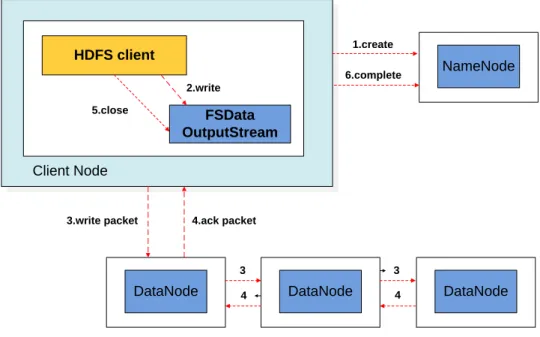
Figure 2.1: Workflow of an HDFS file write operation. . . 11
Figure 2.2: Hadoop job submission. . . 15
Figure 2.3: 5-Level Structure for Spark Application. . . 18
Figure 2.4: Memory Structure in Spark 1.6+. . . 19
Figure 2.5: Representations of Horizontal table and Vertical table. . . 21
Figure 3.1: Workflow of a SMARTH file write operation. . . 24
Figure 3.2: Data Transmission of HDFS . . . 29
Figure 3.3: Data transmission of SMARTH . . . 31
Figure 3.4: Comparison of uploading time on different clusters with and without network throttling. . . 36
Figure 3.5: Comparison of small instances’ uploading time when throttled bandwidth between two racks varies. . . 37
Figure 3.6: Comparison of medium instances’ uploading time when throttled bandwidth between two racks varies. . . 38
Figure 3.7: Comparison of large instances’ uploading time when throttled bandwidth
be-tween two racks varies . . . 38
Figure 3.8: Relationship between bandwidth throttling and performance improvement. . . 39
Figure 3.9: Comparison of small instances’ uploading time when the number of nodes with 50Mbps throttling varies. . . 41
Figure 3.10:Comparison of uploading time for medium and large clusters when the num-ber of nodes with 50Mbps throttling varies. . . 41
Figure 3.11:Comparison of uploading time for small and medium clusters when the num-ber of nodes with 150Mbps throttling varies. . . 42
Figure 3.12:Comparison of uploading time of different data size in a heterogeneous cluster. 43 Figure 4.1: Resource request in Hadoop. . . 47
Figure 4.2: Resource request in D+ Mode of MRapid. . . 48
Figure 4.3: Hadoop’s Uber mode. . . 52
Figure 4.4: U+ Mode in MRapid. . . 53
Figure 4.5: Speculative execution in MRapid. . . 54
Figure 4.6: WordCount performance when varying the number of files but fixing the file size to 10MB. . . 59
Figure 4.7: WordCount performance by fixing the number of files to 4 but varying file size. 60 Figure 4.8: WordCount performance when fixing the input size to 60 MB. . . 61
Figure 4.9: TeraSort performance with different numbers of rows. . . 62
Figure 4.10:PI performance when varying the number of seeds. . . 63
Figure 4.11:WordCount performance when varying the number of containers for each core. 64 Figure 4.12:WordCount performance with different numbers of nodes. . . 65
Figure 5.1: System Architecture of Hedgehog. . . 68
Figure 6.1: Gradient Descent with Iterative Local Search. . . 78
Figure 6.2: Accuracy of different numbers of local iterations in every global iteration. . . 85
Figure 6.3: Performance of different numbers of local iterations. . . 86
Figure 6.4: Data distributions with different scaling factor. . . 87
Figure 6.5: Accuracy of different scaling factor . . . 87
Figure 6.6: Performance with and without adaptive learning rate. . . 88
Figure 6.7: Performance of different input data sizes. . . 89
Figure 6.8: Performance of different initial learning rate . . . 90
Figure 6.9: Performance of different minibatch rate. . . 91
Figure 6.10:Two datasets with different distributions. . . 92
Figure 7.1: System architecture of Dart. . . 95
Figure 7.2: Data distributions. . . 105
Figure 7.3: Performance comparison of calculating mean and median. . . 106
Figure 7.4: Performance comparison between mean and median. . . 108
Figure 7.5: Results of KNN and Distribution. . . 109
LIST OF TABLES
Table 3.1: Amazon EC2 instance types . . . 35
Table 4.1: Notations used in the estimation algorithm . . . 56
Table 4.2: Microsoft Azure instance types. . . 58
CHAPTER 1: INTRODUCTION
The proliferation of massive datasets and the surge of interests in big data analytics have popular-ized a number of novel distributed data processing platforms such as Hadoop and Spark. How to optimize the performance of big data platforms is a big challenge to a system user.
Figure 1.1: Structure of distributed computing platform.
The performance analysis technology for big data platform is the key to explore the hidden value in the big data. The traditional analysis method is to investigate the log information generated by the original big data platform after execution, detect and improve performance bottleneck. But such a method cannot effectively solve complex problems. Therefore, we stratify a big data system into four layers: storage layer, resource management layer, computing layer, and methodology layer, as shown in Figure 1.1 and improve their performance separately. The dissertation is organized based on the optimizations we designed for these four layers.
1.1 Storage Layer
The storage layers employs Hadoop Distributed File System (HDFS), a distributed file system in Hadoop, to store the input and output data for applications. Hadoop provides a distributed, scalable, and portable file system written in Java for the Hadoop framework, called HDFS. There are some major differences from other distributed file systems,e.g., highly fault-tolerant, and can be easily deployed on low-cost hardware. Due to the partitioning of data across commodity hosts, Hadoop can easily distribute computation with tens of thousands of servers in a cluster.
Like other distributed file systems like PVFS, and GFS, HDFS stores input data and file metadata separately as a master/slave architecture. Metadata are stored in a specific server called NameNode; application data are stored across multiple machines called DataNodes. For reliability, these input files are replicated three copies by default.
HDFS contains a single namenode that manages the entire file system, and one or more datanodes serve read and write requests from client systems. HDFS assumes that all nodes in a cluster are ho-mogeneous and can process requests with similar speed. However, in real world, the performance of (e.g., network, disks, and CPU) nodes could be different from one another due to various reasons, e.g., different generations of hardware, different virtual resource allocation, resource contention in virtualized environments. We found that this disparity in performance amongst datanodes within an HDFS cluster can significantly hamper its write performance when handling upload of data files from client local file system, especially when the storage cluster is configured to use replicas.
Therefore, we propose an asynchronous multi-pipeline file write protocol called SMARTH to re-place the traditional stop-and-wait protocol in HDFS [2]. Instead of transferring data blocks one by one and waiting forACK(acknowledgement) packets from all datanodes involved in the transmis-sion, SMARTH (Smart HDFS) builds a new pipeline after it finishes sending the current block to
the first datanode in the pipeline so that it can start sending the next data block right away. This new design makes better use of the network capacity of the client as well as the datanodes’ accessing bandwidth within the cluster. In order to minimize the time of the file importing process, we intro-duce a flexible sorting algorithm of datanodes based on real-time and historical datanode accessing status (including network and storage I/O). We employ the heartbeat mechanism to report the data transmission speed on each client to the namenode every three seconds. Based on the collected information, the namenode can give a good estimate of which set of datanodes a client should use for best performance. When the replication factor of an HDFS cluster is greater than one, which is often used in production environments, we optimize the way that a client interacts with each of the datanodes in a pipeline to allow additional parallelism in data transfer. However, this also changes the way that HDFS ensures data fault tolerance, and thus, we revise its fault tolerance method so that the new way is compatible with the asynchronous multi-pipeline protocol.
We simulate various network conditions using bandwidth throttling on Amazon EC2, we demon-strate that the asynchronous multi-pipeline algorithm is able to remove the single pipeline barrier and effectively overlap data transfer in different pipelines for HDFS file write operations. Over-all, SMARTH is able to improve the throughput of data transfer by 27- 245% in a heterogeneous virtual cluster of Amazon EC2.
1.2 Resource Management Layer
Resource Management Layer is a resource management platform that allows multiple data pro-cessing engines such as interactive SQL, real-time streaming, data science and batch propro-cessing to handle data in a single platform. Here we employ Hadoop Yarn for managing computing resources in Hadoop cluster. The fundamental idea of Hadoop Yarn is to separate the resource management and computation process into different daemons. One of the most significant benefits is that we can
execute different computing engines such as MapReduce and Spark in the same platform without interference.
In the YARN architecture, ResourceManager (RM) usually runs on a dedicated machine and sup-ports High Availability (HA) by running one or more RMs in Standby mode. The RM monitors the status and available resources of DataNodes and assign resources among users’ applications. The RM also decides how to allocate resources among multi-tenants by different kinds of scheduling algorithms.
However, we found that the original Yarn is inefficient and exists some performance bugs, espe-cially for short job. Although Hadoop is designed to process very large data sets, a majority of jobs are short in the real world. For example, the MapReduce jobs at Google in 2004 took 634 seconds on the average, and over 80% of Yahoo’s jobs finished within 10 minutes [3][4][5]. This is mainly due to the input data size being small, especially when it is spread across the entire HDFS cluster and processed in parallel. Moreover, SQL-like query systems, such as Pig and Hive, that operate on top of MapReduce could break a longer running job into a collection of shorter jobs [6][7]. More recently, Uber mode was introduced in Hadoop 2 to specifically deal with jobs with small input size (less than 1 data chunk, to be precise). This special mode runs all tasks of a job within one container. However, even Uber mode is not efficient enough to handle small jobs. We summarize the inefficiencies of running short jobs on Hadoop as follows:
• Hadoop scheduler does not take data locality into account for short job, thus unnecessary data transfer could significantly slow down the execution of short jobs.
• One-time task setup and tear down overheads, which are often negligible in a long running job, can no longer be overlooked for short jobs.
scalability, but waiting a few seconds here and there adds up quickly. Short-circuiting these paths can be beneficial for short jobs.
• In Uber mode, running all tasks sequentially within a single container does not take full advantage of all local resources.
• Moreover, in Uber mode, intermediate data incur disk I/Os, such as spill operation, could significantly degrade performance.
In this study, we propose an efficient short job optimization on Hadoop, calledMRapid, to speed up the execution of MapReduce short jobs [8]. In our system, we design two improved modes based on Hadoop: Improved Distributed (D+) mode and Improved Uber (U+) mode. Our contributions are summarized as follows:
• In D+ mode, we design a new scheduler to schedule Map tasks according to the resource distribution situation and data locality. When an ApplicationMaster requests resources from Yarn, instead of waiting for report from NodeManager, our new scheduler allocates resources according to the current resource availability and data distribution in ResourceManager, and responds the request in the same heartbeat, rather than waiting for at least two heartbeats in Hadoop. Our algorithm not only avoids load imbalance problem for short jobs, but also reduces the communication cost. The benefits of spreading out Map tasks and data-locality awareness are significant, especially when a short job can be executed in one wave.
• In U+ mode, rather than executing Map tasks sequentially, we run multiple Map tasks in parallel on the same node. The degree of parallelism depends on the available resources on the node.
• We design a job submission framework, which reserves an ApplicationMaster pool for reuse and avoids the long waiting time to initialize new ones for short jobs.
• For a short job, deciding which mode (D+ or U+) runs faster is a grand research challenge. Our job submission framework handles it by supporting speculative execution. Specifically, the framework can execute an application initially in both D+ and U+ modes. During the execution, a profiler records the execution and data I/O information for each mode. When the framework is confident that one mode is behind the other, the slower one will be terminated. The winner mode can be designated to the short jobs for the future run.
1.3 Computing Layer
Our Computing Layer provides several software frameworks, such as Hadoop MapReduce and Spark, to process big data applications using certain programming models.
Hadoop MapReduce is a computing model for processing large data sets in parallel. MapReduce paradigm is composed of a Map function that performs filtering and sorting of input data and a Reduce function that performs a summary operation. The input data are always split into several blocks, which are executed simultaneously.
Apache Spark[9] is another open source big data processing framework, which claims that when comparing to Hadoop, it runs up to 100 times faster based on in memory processing and 10 times faster on disk [10].
There are several advantages compared to other distributed computing platform like Hadoop and Storm. First of all, along with in-memory data storage, the performance of Spark is several times faster than other big data platforms. Secondly, instead of just “map” and “reduce”, Spark defines
it also supports many program languages like Java, Scala and Python. Last but not least, it has an abundant ecosystem to support users to write more complex applications easily.
However, when a user submits an application, there are too many parameters to be considered such as the number of cores per executor, memory size per executor, and the number of executors. How to configure these parameters relies on the user’s experience. For instance, considering a case where a cluster contains 10 DataNodes, and each DataNode has 16 cores and 128 GB memory together, we first reserve 1 core and 8 GB memory for OS, Hadoop and Spark. Consequently there are 15 cores and 120 GB per node left to allocate. Then the user can determine how many cores be assigned to each task by “spark.task.cpus”, which is 1 by default. We assume 1 core for each task is reasonable for the user’s application so that the user can execute 15 tasks in parallel in each DataNode. Therefore we can easily calculate how much memory assigned to each task (120 / 15 = 8 GB), however we also need to consider other overheads, so 7 GB per task makes more sense. If 7 GB is not enough for each task, an “out of memory” error will occur, and the user must increase the memory size per task and recalculate the number of tasks per DataNode. Here we assume 7 GB per task is large enough, then decide how many tasks are executed in each executor. Tasks executed in the same executor can share memory and other resource, but too many tasks being processed in the same jvm could lead to poor performance. Here we assume 5 cores per executor is a reasonable configuration. Since we have 15 cores available in each DataNode, 15 / 5 = 3 executors can be allocated in each node, and each executor contains 5×7=35 GB memory.
we propose an efficient 3-level sampling performance model, called Hedgehog, and focus on the relationship between resource and performance [11]. This design is a brand new white-box model for Spark, which is more complex and challenging than Hadoop. In our tool, we employ a Java bytecode manipulation and analysis framework called ASM [1] to reduce the profiling overhead dramatically.
1.4 Methodology Layer
The methodology layer is to carry out complex operations and design a set of API for a specific domain based on the computing layer. Spark is a powerful open-source processing engine which provides abundant APIs for different domains, such as Spark SQL, Spark Streaming, Spark MLlib, Spark GraphX, and SparkR.
In the context of Spark, the driver of a Spark application can be regarded as a specialized parameter server that updates and distributes parameters in a synchronized way. However, unlike parameter server frameworks that are usually implemented on highly efficient MPI, Spark’s synchronous iterative communication pattern is based on MapReduce between the driver and workers, which makes it an inefficient platform for machine learning algorithms using SGD.
Therefore, we design an adaptive fast-turn stochastic gradient descent algorithm, called FTSGD for methodology layer, which works more efficiently on the platforms that rely on iterative commu-nication such as Spark and Hadoop to speed up the convergence of machine learning algorithms, e.g., linear regression, logistic regression, and SVM.
Another API we designed in methodology layer is a spatial analyzing system, called Dart, on top of Hadoop and Spark in purpose of solving spatial tasks like K-nearest neighbors (KNN) and geometric median distribution for social media analytics [12].
In big data computing, Hadoop-based systems have advantages in processing social media data[13]. In this study, we use two geographic measures, the mean center and the median center, to summa-rize the spatial distribution patterns of points, which are popular measurements in geography[14]. The method has been used in a previous study to provide an illustration of social media users’ awareness about geographic places[15]. The mean center is calculated by averaging the x and
sensitive to outliers, which represent a user’s occasional travels to distant places. The median center provides a more robust indicator of a user’s daily activity space by calculating a point from which the overall distance to all involved points is minimized. Therefore, the median center calculation is far more computing intensive. One social media user’s activity space comprises geographic ar-eas in which he/she carries out daily activities such as working or living. The median center thus shows a gravity center of that person’s daily life.
The major advantages of Dart lie in: (1) Dart provides a computing and storage platform that is optimized for storing social media data like Twitter data. It employs a hybrid table design in HBase that stores geographic information into a flat-wide table and text data into a tall-narrow table, respectively. Thus, Dart can get rid of the unnecessary reduce stage for some spatial operations like calculating mean and median centers. Such a design not only cuts down users’ development expenditures, but also significantly improves computing performance. In addition, Dart avoids load imbalance and hot region problems by using pre-splitting technique and uniform hashes for row keys. (2) Dart can conduct complex spatial operations like the mean center and median center calculations very efficiently. Its methodology layer is a completely flexible and totally extensible module, which provides a better support to the upper analysis layer. (3) Dart provides a platform to help users analyze spatial data efficiently and effectively. Advanced users also can develop their own analysis methods for information exploration.
We evaluate the performance of Dart on Amazon EC2[16] with a cluster of 10 m3.large nodes. We demonstrate that our grid algorithm for the calculation of median center is significantly faster than the algorithm implemented by traditional GIS, and we can gain an improvement of 7 times on a 160 GB Twitter dataset and 9 to 11 times on a synthetic dataset. For instance, it costs 1 minute to compute the mean or the median center for 1 million users.
research related to my research work and their limitations. Chapter 3 discusses an innovative asyn-chronous data transmission approach called “SMARTH” is introduced to greatly improve the write operation’s performance in HDFS. We then present an efficient short job optimization on Hadoop, calledMRapid, to speed up the execution of MapReduce short jobs in Chapter 4. In Chapter 5, we propose an efficient 3-level sampling performance model, called Hedgehog, and focus on the re-lationship between resource and performance. We design an adaptive fast-turn stochastic gradient descent algorithm, called FTSGD for methodology layer in Chapter 6. In Chapter 7, another API we designed is a spatial analyzing system, called Dart, on top of Hadoop and Spark in purpose of solving spatial tasks like K-nearest neighbors (KNN) and geometric median distribution for social media analytics. Finally this dissertation is concluded in Chapter 8.
CHAPTER 2: LITERATURE REVIEW
In this section, I briefly review the current research related to my research work and their limitations with regards to the performance improvement for big data systems such as Hadoop and Spark.
This dissertation is related to the four research areas in optimizing performance of a big data platform: (1) HDFS System and Data Uploading; (2) Resource Management and Scheduling; (3) Performance Modeling; (4) Structured Data Store.
` HDFS client Client Node 1.create 2.write 5.close 6.complete NameNode
DataNode DataNode DataNode
3.write packet 4.ack packet
3 3
4 4
FSData OutputStream
2.1 HDFS System and Data Uploading
An HDFS cluster is comprised of a namenode and one or more datanodes. In this section, we give a comprehensive analysis about how a client communicates with the namenode and datanodes when uploading data to HDFS. As shown in Figure 2.1, there are 6 steps to upload data from a local file system into HDFS.
1. Creating a file into the file system’s namespace. The client first makes acreate()HDFS call, which results in a ClientProtocol RPC being invoked to create a new file on the namenode. Before the creation of the file in the namespace, the namenode conducts several checks,e.g., whether the file already exists, whether the user has the right to create the file, and whether safe mode is disabled. If all these checks pass, the namenode would create the corresponding file in the file system’s namespace; otherwise it would throw an exception. 2. Splitting data into packets and inserting into a data queue.To write data to HDFS, client
applications consider the data file as a standard output stream. This data stream is fragmented into blocks, each of which has a default size of 64MB. In turn, each block is split into 64KB packets by default when being transmitted onto the network. When the client writes a new block, aDataStreamerthread would send anaddBlock()call to the namenode to ask for a new block ID and the datanode IDs to store the block. After the corresponding packets are generated, the client sends these packets to a FIFO queue and then to the datanodes.
3. Sending packets to Datanodes. DataStreameruses the datanode IDs to build a pipeline between the client and these datanodes, streams the packets to the first datanode in the pipeline one by one, and stores these packets into another queue called ACK queue in case some datanodes require retransmitting due to packet loss. When the first datanode receives a packet, it verifies the packet’s checksum, stores the packet, and transfers it to the next
datan-ode in the pipeline. This procedure will repeat until the packet reaches the last datandatan-ode at the end of the pipeline.
4. Sending acknowledgement (ACK) back to the client. When the last datanode obtains
the packet, it would send an ACK through the pipeline in a reverse order. The client has a thread calledPacketResponder that is responsible for receiving response ACKs. If the PacketResponderthread receives a packet ACK from all datanodes, it removes this packet from the ACK queue.
5. Closing the output stream. When the client has flushed all data into the output stream, it callsclose()on the stream, and waits for all packets’ ACKs.
6. Completing file write. When all packets’ ACKs are received by the PacketResponder thread, it wakes up the client. The client would send a complete signal to the namenode to complete this file write operation.
In Steps 3 and 4, the client has to wait until it received all ACKs through the pipeline, during which the client could not optimally make use of network capacity.
Although a rich set of research has been published on improving the performance of Apache Hadoop nowadays, there is little work in literature to analyze and improve the file transmission paradigm in the HDFS architecture. Xu et al.[17] tries to figure out a cost model to describe the data import and verify this cost model with practical evaluations. In their approach, Instead of opening an input stream to the local file and passing it along to the first datanode through a socket, the original data storage can be directly accessed by datanodes.
There are some literatures related to file write that mainly focus on adjustments to Hadoop param-eters and codes to adapt HDFS to a specific scenario. For instance, Shafer et al. [18] analyze the
in inefficient HDFS usage. Their paper focuses on adjustments of Hadoop parameters to boost the overall efficiency of MapReduce applications. CoHadoop[19] is a lightweight extension of Hadoop that controls where data are stored. It uses hints given by applications to locate data files to improve efficiency. HDFS+[20] is an extended distributed file system from existing HDFS that can accept concurrent writes with multi data sources. In HDFS+, files are divided into fragments not sent in a sequence order, instead, each fragment can be written individually by a client.
A number of other research work have been proposed to make Hadoop more efficient than the original Hadoop. Islam et al.[21] introduce a novel design of HDFS using Remote Direct Memory Access (RDMA) on InfiniBand. The design is able to provide low-latency and high throughput for HDFS write operations as it leverages the RDMA capability of high performance network like InfiniBand. Yee et al.[22] introduce a generic socket API called Hadoop Filesystem Agnos-tic API (HFAA) to allow Hadoop to integrate with any distributed file system over TCP sockets. This socket API can eliminate the demand to customize Hadoop’s Java implementation, and move the implementation responsibilities to the file system. Hadoop-A[23] introduces a novel network-levitated merge algorithm to merge data without repetition and disk access to optimize data pro-cessing throughput of Hadoop.
2.2 Resource Management and Scheduling
Yarn, a cluster resource manager, is a key component of Hadoop 2, and MapReduce is one of computing frameworks that runs on Yarn. In this section, we give a comprehensive overview of the job submission process. As shown in Figure 2.2, there are 6 steps to submit a job.
Figure 2.2: Hadoop job submission.
1. Job Submission:To submit a new job, a client first communicates with the ResourceManager (RM) to generate a new job ID. which in turn checks the specification of the job, uploads input splits, job Jar file, and configuration to HDFS. The client then submits the job to the RM.
2. ApplicationMaster (AM) Allocation: When the RM receives the job submission request, the scheduler allocates a container to set up and launches an AM instance.
3. Launching AM:The designated NodeManager (NM) of the allocated container launches AM for the job. Once AM is started, it downloads input splits, job Jar file, and configuration from
HDFS, and initializes itself.
4. Request Containers: If the job is not configured to run in Uber mode, the AM requests containers for Map and Reduce tasks from the RM, which schedules resources based on data locality that allocates each task to be near its input data. Hadoop employs CapacityScheduler by default, which allows multiple tenants to share a large cluster and allocate resources under constraints of specified capacities for each user.
5. Task Assignment: After tasks have been assigned to run in certain containers by the RM’s scheduler, the AM starts the containers by contacting the corresponding NMs.
6. Task Execution: After downloading configuration and Jar file from HDFS, the Map or Re-duce task is executed as a Java application in JVM.
Submitting job in Hadoop system is inefficient and time-consuming due to creating containers and piggybacking requests and responses to transfer periodic heartbeat messages.
There are four research areas in optimizing performance related to our research: short job schedul-ing [5, 24, 25], data-locality awareness [26, 27, 28], cache mechanism [29], and reusschedul-ing resource [30].
Elmeleegy [5] designed a system called Piranha that avoids checkpointing intermediate results to disk. It also supports a simple fault-tolerance mechanism, and employs self-coordination to reduce the cost of high-latency polling protocol. However, this system reduces only cost of spilling data into disk, and the Uber mode is not considered. Yaoet al.[24] propose a job-size based scheduling algorithm. It leverages the knowledge of workload patterns to reduce average job response time by dynamically tuning the resource sharing among users. But this approach cannot reduce useless overhead caused by Hadoop itself. Yan et al. [25] implement an optimized version of Hadoop
pull-model task assignment mechanism with a push-model approach. This system just reduces the communication between Driver to NameNode and JobTrack to TaskTrack, but cannot reuse previous jobs’ execution environment to speed up.
Hammoudet al. [26] designed a Locality-Aware Reduce Task Scheduler (LARTS), which collo-cate Reduce tasks with the maximum required data after recognizing input data locations and sizes. This method is useful only when the input data are skewed, and the performance improve is not significant. Zhanget al. [27] proposed a next-k-node scheduling (NKS) method to reserve nodes for Map tasks to satisfy node locality policy. It is not enough for short job by just considering data locality. Maestro [28] is another scheduling algorithm that schedules map tasks in two waves: first, it fills the empty slots of each data node based on the number of hosted map tasks; second, runtime scheduling takes into account the probability of scheduling a map task depending on the replicas of the task’s input data. But for many short jobs, there is only one wave to be executed.
Spark [31][32] is a fast and general engine that can be deployed on Hadoop Yarn. It organizes data into a distributed data structure called resilient distributed dataset (RDD), which can be cached in memory, and be reused across different computations. But we observed that the performance of Spark on Yarn is still slow for short jobs because of the high overhead to launch containers for AMs and executors.
HJ-Hadoop [30] is designed to exploit multicore parallelism at the intra-JVM level, while limiting the number of JVMs created on each node. In our U+ mode, we employ a similar technique, which executes Map tasks of a container in parallel rather than a sequential way.
Besides optimizing MapReduce performance, Hadoop can be improved in many other aspects, such as network [33], HDFS [2], middleware [34], and query optimization [12].
2.3 Performance Modeling
A Spark program includes 5 hierarchical levels: application, job, stage, task, and operation, which is shown in Figure 2.3. Instead of having job as the highest level in Hadoop, the highest level for Spark is application, which is submitted by a client to the resource manager and is launched in an ApplicationMaster container. An application can contain more than one jobs, the number of which depends on the number of actions,i.e., each action is executed by a job.
RDD 0 RDD 1 RDD 2 Stage 0 Stage 1 Job 0 Task 0 Task 1 Task 2 Task 3 Job 1, … … Application Shuffle
Figure 2.3: 5-Level Structure for Spark Application.
On the application level, all jobs are merged into one package, which makes it easier to design and more efficient to execute a recursive application such as machine learning application. Each job is triggered by one action, which always returns the result to the driver. In each job, due to the number
of shuffling operations, it can be divided into many stages. Spark must shuffle data between two neighboring stages, which is also called wide dependency. A stage may contain multiple tasks, each of which handles one partition of data. Each RDD usually consists of many partitions, thus multiple tasks in each stage may run in parallel on compute nodes. For each task, it still executes several narrow dependent operations, which indicates that operations are executed like pipelining without network shuffling. The lowest level is operation. In general, the lower the level is, the less execution information Spark collects since the overhead is more expensive.
sp ark.memo ry .fr actio n 60% Storage Memory Execution Memory
User Managed Memory Spark Managed Memory spark.memory.storageFraction
(50%)
Figure 2.4: Memory Structure in Spark 1.6+.
Ever since Apache Spark version 1.6.0, Spark memory is divided into three regions to manage: user memory, storage memory, and execution memory [35], as shown in Figure 2.4. User memory completely depends on the user-defined function. The quality and feature of the user code has direct effection on this part of memory usage. Storage Memory is used for both cached data and “broadcast” variables. This type of memory is related to data reusing and broadcasting. Execution Memory stores the intermediate shuffling data on both Map side and Reduce side. The boundary
between the storage memory and the execution is not fixed, which means if one kind of memory is insufficient, it can borrow space from the other. How to decide the memory fraction for each memory region is a very challenging problem since the memory usage is totally case by case, and there are so many influencing factors making it hard to analyze.
Starfish [36] is a white-box performance model for Hadoop, which instruments the application and builds the relationship between execution performance and configurations by formulas. However, the overhead of the instrumentation method is too expensive, furthermore, its covering for wide-range applications and formalization makes it inaccurate for some types of applications. There are other existing researches to analyze the performance model but typically not focus on the internal structure and comprehensive process analysis [37, 12, 38, 39, 8].
2.4 Structured Big-data Store
Efficient management of social media data is important in designing data schema. There are two choices when using NoSQL database: tall-narrow, or flat-wide[29]. The tall-narrow paradigm is to design a table with few columns but many rows, while the flat-wide paradigm is to store data in a table with many columns but few rows. Figure 2.5 shows a tall-narrow table and its corresponding realization in the flat-wide format.
For a flat-wide schema, it is easy to extract a single user’s entire information in a single row, which can easily fit into a MapReduce program. For a tall-narrow table, each row contains a single record of a user’s entire information to avoid data imbalance layout and too much data stored in just a single row.
Key Q1 Q2 Q3
u1 a Null b
u2 Null c Null
u3 Null b a
u4 b Null Null
Key Qualifier Value
u1 Q1 a u1 Q3 b u2 Q2 c u3 Q2 b u3 Q3 a u4 Q1 b
Figure 2.5: Representations of Horizontal table and Vertical table.
For sparse data, the tall-narrow table is a common way and can support e-commerce type of ap-plications very well[40]. In addition, HBase only splits at row boundaries, which also contributes to the users’ choice of tall-narrow tables[29]. Using a flat-wide table, if a single row outgrows the maximum of a region size, HBase cannot split it automatically, which makes data stored in that row overloaded.
In our system, we employ a hybrid schema, in which we store geographic data by a flat-wide table, and store other data like text data by a tall-narrow table. Since numerical location information is significantly smaller than text data, each user’s location data can easily fit into a region size (256M by default). Our design can make complex geographic operations more efficient due to removing the reduce stage from a MapReduce job.
Some GIS over Hadoop and HBase have been designed to provide convenient and efficient query processing. However, they do not support complex queries like geometric median. A few systems employ Geographic Index like grid, R tree, and Quad tree to improve the processing, which are,
unfortunately, not helpful for calculating geometric median efficiently.
SpatialHadoop[41] extends Hadoop and consists of four layers: language, storage, MapReduce, and operations. The language layer supports a SQL-like language to simplify spatial data query. The storage layer employs a two-level index to organize data globally and locally. The MapReduce layer allows Hadoop programs to exploit index structure. The operations layer provides a series of spatial operations like range query, KNN, and join. Hadoop-GIS[42] is a spatial data warehousing system that also supports a query engine called REQUE, and utilizes global and local indexes to improve performance. MD-HBase[43] is a scalable data management system based on HBase, and employs a multi-dimensional index structure to sustain an efficient insertion throughput and query processing. However, these systems are incapable of offering a good data organization structure for social network like Twitter, and their index strategies cannot calculate the geometric median efficiently due to an extra load on data management, index creation and maintenance.
CG_Hadoop[44] is a suite of MapReduce algorithms, which covers five different geometry spatial operations, namely, polygon union, skyline, convex hull, farthest pair, and closest pair, and uses the spatial index in SpatialHadoop [41] to achieve good performance. Zhang et al. [45] implements several kinds of spatial queries such as selection, join, and KNN using MapReduce and proves that MapReduce is appropriate for small scale clusters. Lu et al. [46] designs a mapping mechanism that exploits pruning rules to reduce both the shuffling and computational costs for KNN. Liu et al. [47] employs the MapReduce framework to develop a scalable solution to the computation of a local spatial statistic (G∗i(d)). GISQF[48] is another spatial query framework on SpatialHadoop [41] to offer three types of queries, Longitude-Latitude Point queries, Circle-Area queries, and Aggregation queries. Yet, there is no operation or discussion for calculating geometric median on top of Hadoop and HBase.
CHAPTER 3: ENABLING MULTI-PIPELINE DATA TRANSFER IN
HDFS
In this work, we introduce an improved HDFS design called SMARTH1. It utilizes asynchronous multi-pipeline data transfers instead of a single pipeline stop-and-wait mechanism. SMARTH records the actual transfer speed of data blocks and sends this information to the namenode along with periodic heartbeat messages. The namenode sorts datanodes according to their past perfor-mance and tracks this information continuously. When a client initiates an upload request, the namenode will send it a list of “high performance” datanodes that it thinks will yield the highest throughput for the client. By choosing higher performance datanodes relative to each client and by taking advantage of the multi-pipeline design, our experiments show that SMARTH significantly improves the performance of data write operations compared to HDFS. Specifically, SMARTH is able to improve the throughput of data transfer by 27-245% in a heterogeneous virtual cluster on Amazon EC2.
3.1 Asynchronous Multi-pipeline Protocol
In the original HDFS design, when a client wants to write a data block to an HDFS cluster, it receives a list of datanodes from the namenode to form a pipeline. The data block travels from the client to each of the datanodes sequentially, and the client will only mark a block as completed when the ACK packets from all the datanodes in the pipeline are received. Therefore, the effective bandwidth of the pipeline is limited by the slowest datanode in the pipeline.
1The content in this chapter was in part reproduced from the following article: Hong Zhang, Hai Huang, Liqiang Wang, SMARTH: Enabling Multi-pipeline Data Transfer in HDFS, 43rd International Conference on Parallel Process-ing, 2014. The copyright form for this article is included in Appendix A
` FSData OutputStream Client Node 1.create 2.write 5.close 6.complete NameNode
DataNode DataNode DataNode
3.write packet
4.ack packet
3 3
4 4
DataNode DataNode DataNode
3 3 4 4 4.ack packet PipeLine2 PipeLine1 HDFS client
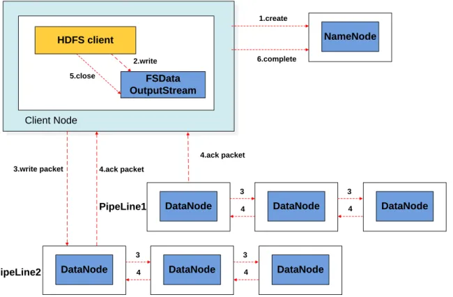
Figure 3.1: Workflow of a SMARTH file write operation.
The way that SMARTH handles data write operations is shown in Figure 3.1. Step 1 is similar to Hadoop. When the client writes a block, it first asks for a block ID and a list of datanodes to store the data. The SMARTH namenode then chooses a high-bandwidth node relative to the client as the first datanode in the pipeline (based on historical information, which we will describe later). In step 2, the client splits data blocks into same size packets and puts them into a data queue.
During data transmission, the client sends these packets to the first datanode, and after storing them locally, this datanode forwards them to the second datanode and so on and so forth until the
last datanode receives all the packets (step 3). When the first datanode receives all the packets of a certain block, it sends back a special ACK packet calledFIRST_NODE_FINISH_ACK (FNFA)to the client. This packet indicates to the client that the entire block has been received and stored by the first datanode in the pipeline. Instead of waiting for ACKs from the other datanodes, the client continues to send the next data block by requesting another block ID and datanodes from the namenode. This results in a new pipeline being formed for sending the next data block. Additional pipelines can be formed if the client can send packets to the first datanode quicker than the speed that the packets travel to the other datanodes in the pipeline.
After creating a pipeline, we create an ACK queue and a PacketResponder thread for it. Each pipeline transfers ACKs back to the corresponding PacketResponder thread (step 4). As the PacketResponderthread receives an ACK from its pipeline, it removes the corresponding packet from its ACK queue. At the client, we use a set to enumerate all active pipeline objects. When the PacketResponderthread receives all ACKs, it will be removed from this set. When the pipeline set is empty, we close output stream (step 5) and complete this uploading (step 6).
Using this method to upload files to HDFS, the client can fully utilize its bandwidth capacity and reduce idle time on waiting for ACK messages. Thus, the speed of the asynchronous pipeline transmission is now determined not by the minimum bandwidth amongst client and datanodes but the network speed between the client and the first datanode in the pipeline. In the following subsections, we describe how SMARTH namenode finds the “best” first datanode for each client while keeping the cluster balanced.
3.2 Global Optimization for Data Transmission
Traditional HDFS represents a network topology as a tree structure [49]. When the client requests a list of datanodes for storing a data block, the namenode chooses the target nodes according to this network topology tree,e.g., to optimize for performance and to maximize data fault tolerance. However, it cannot accurately capture the real-time network condition as this information is usually not directly correlated with the network topology.
In SMARTH, client records the transmission speed of data blocks to all the first datanodes in transfer pipeline that it had communicated before and sends these records to the namenode every three seconds by remote procedure calls (RPCs), following the default heartbeat mechanism in Hadoop. When the client subsequently requests datanodes to place additional data blocks, the namenode utilizes this information to choose a set of best performing datanodes in the cluster according to our global optimization algorithm shown below.
Algorithm 3.1 describes SMARTH namenode’s global optimization algorithm for choosing datan-odes. When the namenode receives a request to upload files from a client, it calculates the maxi-mum number of pipelines allowed for the client, and assign it to a variablen. Our design selects a datanode randomly from thenbest performing nodes for this client as the first datanode so that we can guarantee the bandwidth between the client and the first datanode is relatively higher in the pipeline. The second replica is selected from a different rack and the third replica is placed on the same rack as the second.
Algorithm 3.1Algorithm for global optimization
1: num= the number of active datanodes
2: repli= the number of replica factor
3: n=num/repli//the maximum pipeline size
4: if (namenode has transmission records for the client) then
5: TopN = top n datamodes in terms of transfer speed
6: // the number of datanodes we have choosen
7: results= 0
8: while (results!= repli) do
9: if (results== 0) then
10: targets[0] = randomDatanode(TopN)
11: else if (results == 1) then
12: targets[1] = randomRemoteRackNode()
13: else if (results == 2) then
14: targets[2] = nodeOnSameRack(targets[1])
15: else
16: targets[results] = randomDatanode()
17: end if
18: results++
19: end while
20: else
21: targets= employ the original HDFS method to select datanodes
22: end if
3.3 Local Optimization for Data Transmission
Since network status varies all the time, we utilize a local optimization algorithm to sort the datan-odes order in pipeline by the newly records and give a chance to test the bandwidth performance of nodes with poor performance previously.
Algorithm 3.2 shows details of local optimization algorithm executes in the client node. We use block transfer records locally to calculate the transmission speed for each datanodes assigned to TransSpeed, and employ sort algorithm to reorder the targets set. We calculate a random number rbetween 0 to 1 to decide whether to swap the first datanode with another datanode in pipeline so that we can update the transmission records of that node. In this way, we may keep transmission
Algorithm 3.2Algorithm for local optimization
1: repli= the number of replica factor
2: TransSpeedVector= the transmission speed of every nodes intargets 3: sorttargetsin descending order byTransSpeedVector
4: r= a random number between 0 to 1
5: if (r>threshold) then
6: //the target index to switch the first datanode 7: index= a random integer between 1 torepli−1
8: swap(targets[0],targets[index])
9: end if
information for all datanodes updated occasionally. In our algorithm, ifris greater thanthreshold that is assigned to 0.8, we use another random integer indexto choose which datanode to switch with the first one.
3.4 Cost-Benefit Analysis
To pinpoint how SMARTH outperforms HDFS, we analyze a file write operation in details and compare the two designs step by step. Data transfer between a client and datanodes for the original HDFS is shown in Figure 3.2. When the number of replica is greater than one, datanodes will forward each packet to the next datanode along the pipeline until the last datanode receives it. Client will wait for ACKs from all datanodes in the pipeline before it can start sending the next data block.
Client Datanode1 Datanode2 Datanode3 data ACK Namenode Communicate Data queue Create packets ACK queue Network
Figure 3.2: Data Transmission of HDFS
Assume that data file size isD, block size isB, and data file size is greater than one block, the file is split intopD/Bqblocks. Assume that the packet size isP, the number of packets transferred is pD/Pq.
Let Tn denote the communication time between client and namenode for each block. Let Tc de-note the average production time (read data from local file, compute the checksum and append the data and checksum to a packet) for a packet by the client. When the datanode receives a packet,
it verifies the checksum and writes the packet to the local disk that takes Tw on average. Let Bmin represent the minimum bandwidth between client and the first datanode and amongst adja-cent datanodes. Since the size of ACK packets is smaller than the data packets, and the time of transferring ACKs and the time of sending data packets overlaps, we only need to take the packet transmission time into account.
As the production and the transmission of packets are executed by different threads, there is an overlap between the production time and the transmission time of packets. If the average pro-duction time of packets is greater than or equal to the average packet transmission time along the pipeline, there is no packet waiting for sending on data queue. The total production time for all packets is the major factor to the whole importing time. In this scenario, Tc>=P/Bmin, and the total time consuming is shown in Formula (3.1). However, even in the small instance, to produce a packet is very fast compared with the speed to send a packet in our experiments.
T =Tn∗pD/Bq+ (Tc+Tw)∗pD/Pq (3.1)
If the packet production time is less than the packet transmission time, there must exist blocking on data queue. So the total cost relies on the minimum bandwidth amongst client and datanodes. In this scenario,Tc<P/Bmin, and Formula (3.2) shows the total time consuming.
T =Tn∗pD/Bq+ (P/Bmin+Tw)∗pD/Pq (3.2)
From the analysis above, we know that the time of importing file is determined by the production time or the transmission time of packets, depending on which is larger.
data FNFA Network Data queue Create packets ACK queue
Client Datanode1 Datanode2 Datanode3
Namenode Communicate
ACK
Figure 3.3: Data transmission of SMARTH
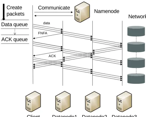
Figure 3.3 shows the process of data transmission for SMARTH. When the first datanode receives all packets of a block, it sends a FNFA back to the client, and the client can then create a new pipeline to prepare for transmitting the next block. Assume the bandwidth between the client and the first datanode is Bmax. If the average production time of packets is greater than or equal to the packet average transfer time from the client to the first datanode (Tc>=P/Bmax), the speed of seeding a packet is slower than the speed of producing a packet. Then there is no blocking in data queue, and the total time consuming is as Formula (3.1) shown.
client to the first datanode (Tc<P/Bmax), the total cost relies on the bandwidth between the client to the first datanode as Formula (3.3) shows.
T =Tn∗pD/Bq+ (P/Bmax+Tw)∗pD/Pq (3.3)
It is obvious thatBmax is greater than or equal toBmin. So our improved HDFS is more efficient than the existing one. We can also find out that idle time waiting for ACK is reduced when we compare Figure 3.2 with Figure 3.3.
3.5 Fault Tolerance
3.5.1 Fault Tolerance for Original HDFS
Since Hadoop is often deployed on a large cluster of commodity nodes, being able to automatically handle faults is a crucial part of its design. This section provides an overview of the fault tolerance mechanism in original HDFS and then discusses our own fault tolerance approach for the multi-pipeline design in SMARTH.
Algorithm 3.3 shows how a typical process handles errors during uploading files to HDFS. When the client catches an error in the process of transmitting a block, it first checks the validity of parameters, and closes all streams related to the block. Then it moves all packets in ACK queue back to data queue. It picks the primary datanode from active datanodes in pipeline, and uses it to recover the other datanodes. If fails, picks another primary datanode and recover again until recovering the block successfully or throwing an exception. At the end, the client recreates the ResponseProcessorthread for receiving remaining ACKs.
Algorithm 3.3Algorithm for fault tolerance of HDFS
1: checks the validity of parameters
2: close all streams related to the block
3: moves all packets in ACK queue back to data queue
4: success= false
5: while (!success) do
6: if (targetsis not empty) then
7: return an exception
8: else
9: primaryNode= the first datanode intargets
10: add new datanodes to replace error nodes intargets 11: success=recoverBlock(primaryNode,targets)
12: if (!success) then
13: remove primaryNodefromtargets
14: end if
15: recreate block streams
16: end if
17: end while
18: recreateResponseProcessorthread
3.5.2 Fault Tolerance for Multi-Pipelines
Since we employ an asynchronous multi-pipeline design, we need to replace the original fault tolerance mechanism with a new design.
Algorithm 3.4Algorithm for fault tolerance of SMARTH
1: stop the current block transfer
2: moves all packets in ACK queue back to data queue
3: while (errorPipelineSet is not empty) do
4: recover one error pipeline as Algorithm 3.3
5: remove the error pipeline fromerrorPipelineSet 6: end while
7: start transferring the interrupted block
Algorithm 3.4 shows our approach to handle the multi-pipeline fault tolerance. When an error occurs in a pipeline, SMARTH adds the error pipeline into an error pipeline set. It firstly stops the current block sending, and starts a recovery process to recover error pipelines in this set. Each
pipeline’s recovery process is similar to the original single pipeline recovery of HDFS. If the error pipeline is recovered, we delete the error pipeline from the error pipeline set. We continue recover-ing error pipeline until the error pipeline set is empty, then the client restart sendrecover-ing the interrupted block.
3.5.3 Buffer Overflow Problem
In SMARTH, since we employ global optimization and local optimization, the first data node is always a high bandwidth node compared with other datanodes. So the client can send data to the first datanode quickly, but the first datanode cannot send packets quickly to the second datanode. Therefore it is possible that the buffer in the first datanode overflows. When the size of data file is large, and the bandwidth varies considerably from node to node, the buffer of the high bandwidth nodes has higher chance for overflow.
We limit the pipeline size to a maximum number ( the cluster size / the number of replica), and if a datanode is already in a pipeline, it cannot be added into other pipelines created by the same client. Then each datanode belongs to only one pipeline, and its buffer is set to be 64 MB,i.e., the default size of block, for each client.
3.6 Experiments
The study was conducted using Amazon EC2’s compute instances. Amazon EC2 supports servers of different types such as small, medium, and large instances. These instances differ in the number of cores, the memory allocated to them, bandwidth, and price (see Table 3.1). An Elastic Compute Unit (ECU) is an EC2-specific unit to express the computational performance of a CPU core. 1 ECU is the equivalent CPU capacity of a 1.0-1.2 GHz 2007 Opteron or Xeon processor.
Table 3.1: Amazon EC2 instance types
Instance Type Memory ECUs Network
Small 1.7 GB 1 ≈216Mbps
Medium 3.75 GB 2 ≈376Mbps
Large 7.5 GB 4 ≈376Mbps
We use four different clusters in our evaluations. Three of the clusters are homogeneous consisted of one namenode and nine datanodes, i.e., of small, medium, or large instances. The other cluster is heterogeneous consisted of 3 small, 4 medium, and 3 large instance nodes, where one medium instance is the namenode and the others are datanodes. Each node runs CentOS Linux Server 6.2 with kernel 2.6.32-220, and the original Apache Hadoop version 1.0.3. We use Amazon EC2 ephemeral storage to store our data file.
Our goal in this study is to evaluate the impact of various network conditions on both HDFS and SMARTH. We employ a Linux utility calledtc, which is used to control network traffic, to limit both ingress and egress bandwidth between VMs.
3.6.1 Two-Rack Cluster Scenario
For a large cluster, a common practice is to employ its nodes across multiple racks, or even across multiple data centers, for load balancing and fault tolerance reasons. Network bandwidth between nodes in the same rack is often greater than the bandwidth between nodes across racks. To con-sistently simulate this behavior (as EC2 does not expose VM’s physical location), we throttle the network bandwidth of nodes usingtc.
The default strategy of HDFS is to place the first replica on the client node itself if the client is a datanode; otherwise, the namenode picks nodes that are not too full or busy. The second replica is
placed on a different rack from the first and the third is placed on the same rack as the second, but on a different node. Although this strategy offers a good reliability, it is at the cost of performance.
(a) default bandwidth in small cluster (b) bandwidth throttling in small cluster
(c) default bandwidth in medium cluster (d) bandwidth throttling in medium clustere
(e) default bandwidth in large cluster (f) bandwidth throttling in large cluster
Figure 3.4: Comparison of uploading time on different clusters with and without network throt-tling.
In our experiments, our file sizes vary from 1GB to 8 GB, and we measure the time to upload the files in both original HDFS and SMARTH using an HDFS put command. We have performed
these experiments on small, medium, and large instances. Figure 3.4(a) and Figure 3.4(b) show that the file size is proportional to the time consumed when importing file to HDFS and SMARTH in small cluster without and with bandwidth throttling of 100 Mbps between two racks. The same conclusion can be also found in medium and large instances from Figures 3.4(c) and 3.4(d), Figures 3.4(e) and 3.4(f). Due to these results, we only consider the input file size is 8 GB in the rest of the paper when we measure the performance of HDFS and SMARTH.
Figures 3.4(c) and 3.4(e) as well as Figures 3.4(d) and 3.4(f) also show that the file importing performance of large cluster is roughly the same with the performance of medium cluster. That is because the medium cluster and large cluster have the same networking capacity. Figures 3.4(a), 3.4(c), and 3.4(e) show that there is no big gain if the cluster’s network status is homogeneous, where network is in the default bandwidth and without throttling.
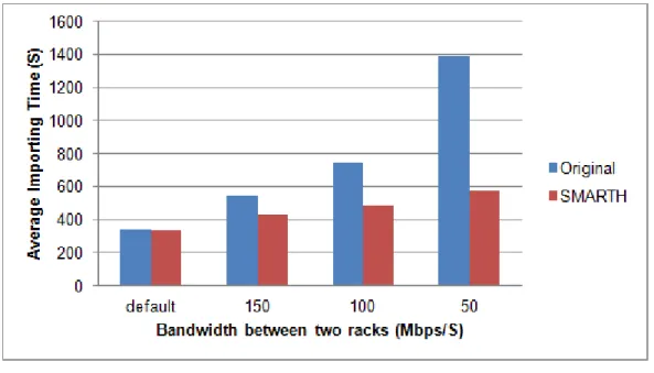
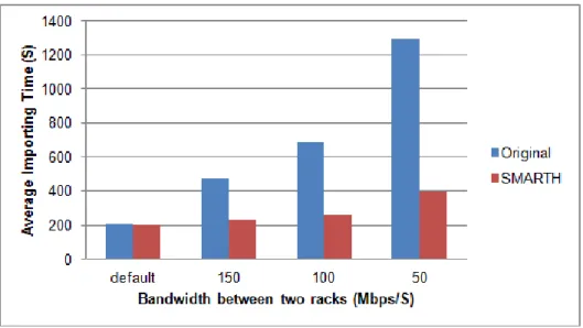
Figure 3.5: Comparison of small instances’ uploading time when throttled bandwidth between two racks varies.
Figure 3.6: Comparison of medium instances’ uploading time when throttled bandwidth between two racks varies.
Figure 3.7: Comparison of large instances’ uploading time when throttled bandwidth between two racks varies
Figure 3.5 shows the file write times on Hadoop and SMARTH when we throttle the network to different bandwidth in a small cluster. As Figure 3.5 shows, the more we throttle the network, the better the performance of SMARTH is compared to HDFS. The new design of SMARTH gains an improvement of 130% when the bandwidth throttling is at 50 Mbps; even when the bandwidth throttling is 150 Mbps, the performance can improve about 27%. We have measured the file write speed in medium and large clusters and observe similar big gains. Figure 3.6 and Figure 3.7 show that SMARTH achieves an improvement of 225% in medium cluster and outperforms HDFS by 245% in large cluster when the network bandwidth is throttled to 50 Mbps.
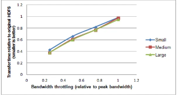
Figure 3.8: Relationship between bandwidth throttling and performance improvement.
Figure 3.8 shows the relationship between how much we throttle the network bandwidth of nodes in small, medium and large clusters and the improvement of SMARTH. The benefit of our design depends on the extent of bandwidth throttling between two racks. When the network bandwidth between nodes in the same rack is much greater than the network bandwidth between nodes in
different ranks, SMARTH can gain more benefit. In a large cluster, where nodes are often allo-cated in different data centers, network performance between a pair of nodes can vary even more significantly within the cluster.
3.6.2 Bandwidth Contention Scenario
In the real world, the bandwidth between nodes in the same rack still varies all the time, and some other procedures also can occupy the bandwidth and contend with Hadoop program. In this scenario, if some nodes with lower network capacity are selected as datanodes to transfer blocks, they can degrade the performance of file write. In SMARTH, we would select the faster nodes as the first datanode and when the first datanode receives the full block, the client builds a new pipeline to continue the file write in order to avoid the idle wait time of the client network and make the best use of the bandwidth between the client and datanodes.
Figure 3.9 shows the time spent during file write when we vary the number of nodes with 50 Mbps throttling from 0 to 5. As shown in Figure 3.9, even there is only one node whose bandwidth is lower than other datanodes, SMARTH can outperform the traditional Hadoop cluster by 78%. We also