On the quasi yield surface concept in plasticity theory

For Peer Review

On the quasi-yield surface concept in plasticity theory

Journal: Zeitschrift für Angewandte Mathematik und Mechanik

Manuscript ID zamm.201600133.R2

Wiley - Manuscript type: Original Manuscript

Date Submitted by the Author: 12-Jan-2017

Complete List of Authors: Soldatos, Dimitris; Demokritos University of Thrace, Department of Civil Engineering

Triantafyllou, Savvas; University of Nottingham,

Keywords: Rate-independent plasticity, quasi-yield surface, integrability conditions, holonomy, large plastic deformations

For Peer Review

On the quasi-yield surface concept in plasticity theory

1

2

Dimitris Soldatos1 and Savvas P. Triantafyllou2

3

1

Department of Civil Engineering, Demokritos University of Thrace, 12 Vasilissis Sofias

4

Street, Xanthi 67100, GREECE 5

2

Centre for Structural Engineering and Informatics, Faculty of Engineering, The University of

6

Nottingham, University Park, Nottingham, NG72RD, UK

7

8

Key words Rate-independent plasticity, quasi-yield surface, integrability conditions, holonomy,

9

large plastic deformations

10

11

In this paper we provide deeper insights into the concept of the quasi-yield surface in plasticity

12

theory. More specifically, in this work, unlike the traditional treatments of plasticity where

13

special emphasis is placed on an unambiguous definition of a yield criterion and the

14

corresponding loading-unloading conditions, we place emphasis on the study of a general rate

15

equation which is able to enforce elastic-plastic behavior. By means of this equation we discuss

16

the fundamental concepts of the elastic range and the elastic domain. The particular case in which

17

the elastic domain degenerates into its boundary leads to the quasi-yield surface concept. We

18

exploit this concept further by discussing several theoretical issues related to it and by introducing

19

a simple material model. The ability of the model in predicting several patterns of the real

20

behavior of metals is assessed by representative numerical examples.

21

22

23

24

For Peer Review

1. Introduction

26

27

In a very recent paper, Xiao et al. [38] posed the question of whether one can construct 28

rate equations which describe rate-independent elastic-plastic behavior, so that it’s 29

essential features, namely the yield criterion and the loading-unloading irreversibility, 30

would not be introduced as extrinsic restrictive conditions, but instead will be derived 31

directly by these equations. In the course of their analysis, Xiao et al. [38], derived a 32

material model which had the ability of simulating several patterns of the real behavior 33

of metals. These patterns comprised - but were not limited to - the prediction of plastic 34

(irreversible) deformations at any stress level no matter how small the latter may be, and 35

a continuous stress-deformation curve at the point of elastic-plastic transition. (For an 36

alternative way of predicting a continuous stress-deformation curve where emphasis is 37

placed in rate-dependent response see the recent works by Hollenstein et al. [11] and 38

Jabareen [12]). 39

Our motivation for this paper is to provide deeper insights into the answer of the 40

question posed by Xiao et al. in [38]. More specifically, in this work, on the basis of 41

some ideas which go back to the classic paper by Lubliner [16] - see also Lubliner in 42

[17,18] - we discuss a purely mathematical approach to elastic-plastic behavior, in 43

which the basic ingredients of plasticity theory follow upon studying the properties of a 44

suitably formulated differential equation. Within this context we pay special attention to 45

a rather old concept, which has passed largely unnoticed within the literature of 46

For Peer Review

The basic steps of this study are as follows: In Section 2, we consider a general 48

differential equation which aims to model rate-independent irreversible response and by 49

means of it and an additional assumption underlying the loading-unloading behavior, 50

we introduce the central concept of advanced plasticity theories, namely the elastic

51

range (see Pipkin and Rivlin [30]; see also Lubliner [19,20]; Luchessi and Podio- 52

Guidugli [24]; Bertram and Kraska [5]; Bertram [4]; Panoskaltsis et al. [27]). Several 53

basic concepts of plasticity such as the loading rate, the elastic domain and the yield 54

surface are also discussed within this framework. In Section 3, we deal with the 55

particular case in which the basic equation is formulated in a way such as the elastic 56

domain is degenerated to its boundary to form a surface; this surface is the 57

aforementioned quasi-yield surface (Lubliner [18,19]). In Section 4, we provide 58

additional insights to the quasi-yield surface concept upon introducing a material model. 59

Finally, in Section 5, we demonstrate the ability of the model in predicting several 60

patterns of the elastic-plastic behavior of metals by means of representative numerical 61

examples. 62

63

64

2. Elastic and plastic processes; elastic range and domain

65

66

As a starting point we assume a homogeneous body undergoing finite deformation whose 67

reference configuration - with points labeled by X - occupies a region B in the ambient 68

space Ω. We define a motion of B in Ω as an one-parameter family of 69

For Peer Review

( ) ( , ), , .

t =

ϕ

t =

ϕ

t ∈B ∈ Ω

x X X X x (1)

71

Then, the deformation gradient is the two-point tensor F, defined as the tangent map of 72

(1), that is 73

: , i.e. i ( , )

iI I

T T B T t

X

ϕ

ϕ ∂

= → Ω =

∂

X x

F F X (2)

74

where T B_X and T_xΩ stand for the tangent spaces at X∈Band x∈Ω, respectively. 75

If one assumes a referential description of the dynamical processes, the local 76

mechanical state over the material point X can be determined by the second Piola-77

Kirchhoff stress tensor S and the internal variable vector Q. We assume that the state 78

(configuration) space S over the point X forms a local (6+Q)-dimensional manifold - 79

where Q is the number of independent components of Q - with points denoted by ( , ).S Q

80

A local process (at X) is defined as a curve in S, that is as a mapping 81

: I S t, ( ( ), ( )),t t

Ψ ∈ → → S Q

82

where I is the time interval of interest. The direction and the speed of the process are 83

determined by the tangent vector Ψ& :S→T ,S with Ψ&( )t =( ( ), ( )),S& t Q& t where TS is the 84

tangent space of S. Since the stress rate (S& =S&( ))t is always known, the component 85

(= ( ))t

Q& Q& of Ψ& has to be determined. The latter may be assumed to be a function of the

86

present values of the state variables and the stress rate, that is 87

( , , ),

=

Q& A S Q S& (3)

88

where A:S×TS →T ,S is a vector field in ,S which may be interpreted as a tensorial 89

function of the state variables. In general, Eq. (3) introduces Q non-holonomic constraints 90

For Peer Review

deal with elastic-plastic (irreversible) response is desirable. However, from a 92

mathematical stand point it may result in integrability problems. In order to surpass this, 93

we further assume that the dependence of Aon S& is linear, that is 94

( , ) : ,

=

Q& L S Q S& (4)

95

where L is a tensor field in .S Motivated by the classical formulations of plasticity - see, 96

e.g. [21, pp. 107,108] - we assume that the function L can be further decomposed as a 97

tensor product as 98

( , )= ( , )⊗ ( , ),

L S Q A S Q ΛΛΛΛ S Q

99

where A is a tensor field and ΛΛΛΛ:S→T S∗ is a one-form, so that Eq. (4) can be expressed 100

as 101

( , )[ ( , ) : ]

=

Q& A S Q ΛΛΛΛ S Q S& (5)

102

We note that Eq. (5) is invariant under a replacement of t by −t and accordingly 103

enforces reversible response (see [29] for further details). On the other hand, plastic

104

behavior is an irreversible one, a fact which calls for an appropriate modification of the

105

rate equation (5). In order to accomplish this goal, we further assume this equation is able 106

of simulating two different types of possible material processes, namely quasi-static and 107

dynamic ones. More precisely, a material process Ψ may be defined as quasi-static if

108

,

=

Q& 0 that is, if it lies entirely in a (6-dimensional) submanifold of S, defined by

109

.;

const

=

Q a non quasi-static process is one which results in a change of the internal 110

variable vector (Q& ≠0) and may be defined as a dynamic process. Herein, the terms

111

quasi-static and quasi-dynamic are being used in complete analogy with classical

112

thermodynamics, see, e.g., [40]. The concept of a quasi-static process leads to the concept 113

of a quasi-static range which is defined at every material state of the material manifold Q

For Peer Review

which comprises all material states (S Q∗, ∗) that can be reached from the current material 115

state ( , )S Q by a quasi-static process, that is 116

{( , ) / , },

Q= S Q∗ ∗ ∈S S∗ = +S dS Q∗ =Q

117

where dS is an infinitesimal stress increment which can be interpreted as a one-form in 118

S. In view of this definition, the quasi-static range can be determined as the union of the 119

submanifolds Q₁ and Q₂ of S, which are defined as 120

1 {( , ) / ( , ) or ( , ) },

Q = S Q∗ ∗ ∈S A S Q∗ ∗ =0 ΛΛΛΛ S Q∗ ∗ =0 (6) 121

where it is implied that the point (S Q∗, ∗) is attainable from ( , ),S Q and 122

2 {( , ) , where ( , ) : 0}

Q = S Q∗ ∗ ∈S S Q∗ ∗ can be attained by a process withΛΛΛΛ S& = (7)

123

As a first step, we disregard the (trivial) cases A S Q( ∗, ∗)=0 and ΛΛΛΛ(S Q∗, ∗)=0 i.e. we 124

assume that A S Q( ∗, ∗)≠0 and ΛΛΛΛ(S Q∗, ∗)≠0,and we focus on the solutions of the 125

equation 126

( , ) :ΛΛΛΛ S Q S& =0 (8) 127

which upon defining the Pfaffian form (see, e.g. [1, pp. 439-444]) 128

:d ,

ω=ΛΛΛΛ S (9)

129

results in the following Pfaffian equation 130

0.

ω= (10)

131

Then if the Pfaffian (one-form) (10) is completely integrable, there exists at the 132

neighborhood of the current material state a scalar function (integrating factor) 133

: S

µ → and a five-dimensional submanifold of S, defined by F( , )S Q =const. - see 134

For Peer Review

( , )=µ( , )∂F.

∂

S Q S Q

S

Λ Λ Λ

Λ (11)

136

The submanifold F( , )E Q =const. is defined - see Eisenberg and Phillips [10]; see also 137

[17,18] - as the loading surface (at Q). Clearly, a process which lies entirely on the 138

loading surface, that is one in which ∂F : =0

∂S S& is a quasi-static one while processes with

139

: 0

F

∂ _≠

∂S S

& are dynamic ones.

140

Rate-independent plasticity - see, e.g., [16] - is closely tied to the concepts of loading 141

and unloading. In order to involve these concepts in the analysis we make the further

142

assumption that a process with ∂F : <0,

∂S S

& results in quasi-static response (Q& =0) and

143

may be defined as elastic unloading, while a (dynamic) process with ∂F : >0,

∂S S

& _which

144

results in Q& ≠0, may be defined as plastic loading. The limiting case ∂F : =0,

∂S S

& _{may be}

145

defined as neutral loading. These concepts can be put together upon replacing the 146

Pfaffian form

ω

in Eq. (5) by a fundamental concept in plasticity theory, namely that of 147

the loading rate -R see, e.g., [16] - which may be defined as

148

: .

F

R=∂

∂S S &

149

Then Eq. (5) can be replaced by

150

( , ) R , =

Q& A S Q (12)

151

where ⋅ stands for the Macauley bracket defined as

2

x x

x = + and it has been 152

For Peer Review

We note that Eq. (12) is invariant under a replacement of t by ( ),ϕ t where ( )ϕ t is any 154

monotonically increasing, continuously differentiable function and accordingly enforces 155

rate-independent response. Moreover, Eq. (12) constitutes the underlying equation of a 156

general model of rate-independent elastic-plastic behavior called generalized plasticity

157

(see Lubliner [20]; see also the later works given in [22,23,26,27,35]). 158

By means of Eq. (12) and by assuming that ∂F( , )≠

∂S S Q 0 in S we can define another

159

fundamental concept, that of the elastic range E - see, e.g., [30,19,20,24] - as the 160

submanifold of S which contains the points which can be reached from the current stress 161

point as 162

.

{( , ) / ( , ) or 0}.

const

E= S Q ∈S A S Q _Q= =0 R≤

163

164

REMARK 1: The present approach, which is based upon postulating a differential

165

equation for the evolution of the internal variable vector and the subsequent derivation of

166

the elastic range by involving the concept of loading-unloading, differs vastly from the

167

standard approaches to the elastic range concept (see, e.g., [20,22,26,27]; see also [3,4]), 168

where the elastic range is considered as a primary concept and the rate-equations are 169

specified afterwards by imposing some regularity requirements and the rate-170

independence property. In this sense, the present approach resembles the general internal 171

variable approach to material irreversible behavior discussed in Lubliner [16]. 172

173

REMARK 2: It is stressed that Eq. (5), although is adequate to define the quasi-static

174

For Peer Review

process with ∂F : <0,

∂S S

& _{is an (elastic) unloading process, that is in such a process the}

176

equality Q& =0 holds; as a matter of fact, this assumption introduces the concept of 177

loading-unloading irreversibility in rate-independent plasticity. 178

179

REMARK 3: Since the present approach involves the stress tensor S and the stress-space

180

loading rate R=∂F : ,

∂S S

& _{presupposes stability under stress control and accordingly is}

181

limited to work-hardening materials. Nevertheless, an equivalent approach which does 182

not suffer from this limitation can be developed within the context of a strain 183

(deformation) space formulation - see, e.g., [21, pp. 120-124]) - if S is replaced 184

throughout by the right Cauchy-Green tensor C, which is defined in terms of the 185

deformation gradient and the spatial metric : g T_xΩ × Ω →T_x as 186

.

= T C F gF

187

It is also noted that the strain-space approach has been proven especially useful- see [27] 188

- for a covariant formulation of the theory of rate-independent plasticity. 189

190

The submanifold D of S

191

{( , ) / ( , ) }

D= S Q ∈S A S Q =0

192

which comprises only elastic processes may be defined as the elastic domain D and its 193

boundary as the yield hypersurface. The intersection of the elastic domain with the 194

submanifold of ,S defined by Q=const., is defined as the elastic domain D_Q (at Q), 195

while its boundary is defined to be the yield surface. Note that unlike the elastic range, 196

For Peer Review

non-connected manifold. Accordingly, the yield surface in this case can be composed of 198

several different independent submanifolds of S, which can be either disjoint, or intersect. 199

We note also that the submanifold of Q₁ defined if ΛΛΛΛ(S Q∗, ∗)≠0 - recall Eq. (6) - is by 200

construction a submanifold of D_Q, but the converse is not necessarily true; this case may 201

appear if the elastic domain is non-connected or contains isolated points which cannot be 202

attained from the current material state. 203

Classical plasticity corresponds to the particular case when an additional constraint, 204

namely the invariance of theelastic domain under a plastic process - see, e.g., [26,27]is 205

introduced in the rate equation (12). If this is the case, the boundary of the elastic domain, 206

i.e. the yield (hyper)surface, coincides with a unique loading (hyper)surface - say defined 207

by F( , )S Q =0 - while the invariance condition (see, e.g., [1, pp. 256-257]) reads 208

0.

GRADF

Ψ ⋅& ≤ ₍₁₃₎

209

where ( )⋅ stands for the inner product in S, and the gradient operator is defined as 210

( ) ( ) ( ) [ , ].

GRAD ⋅ = ∂ ⋅ ∂ ⋅

∂S ∂Q

211

Then, the basic equations of classical rate-independent plasticity - see further [26,27] - 212

can be derived upon assuming that the function Ais of the form 213

( , ) F ( , )

F

=

A S Q B S Q

214

and determining the limit 215

0 0

lim_F ( , ) lim_F F ( , ) ,R F

→ A S Q = → B S Q

216

by means of the limiting case of Eq. (13) where the equality holds, that is 217

:GRADF F( , ) 0

Ψ& = & S Q = (14)

For Peer Review

which constitutes the consistency condition of classical plasticity. 219

An equivalent assessment of the theory in the spatial description can be derived upon 220

performing a push-forward operation (see, e.g., [1, p. 355]; [36]) in Eq. (12). The 221

resulting equation reads 222

( , , ) ,

Lvq=a

ττττ

q F r (15)

223

where , q aare the push-forwards of Qand A in the spatial configuration respectively, 224

ττττ

is the Kirchhoff stress, i.e. = T,

FSF

ττττ and r is the (scalar invariant) loading rate in the 225

spatial configuration r= ∂f :L

∂ vττττ

ττττ where f = f( , , )ττττ q F is the (spatial) expression for the

226

loading surface. In component form, the push-forward operation for the arbitrary tensor 227

Q reads 228

1 1

1 1

1 1 1 1

... ...

... ... ... ... .

n m

n n

m n m m

i J

i J

i i I I

j j I I j j J J

x x X X

q Q

X X x x

∂ ∂ ∂ ∂

=

∂ ∂ ∂ ∂

229

Finally, L_v( )⋅ stands for the (convected) Lie derivative (see further [1, pp. 359-369]; 230

[36]) which is obtained by pullingback q to the reference configuration, taking its time 231

derivative by keeping X fixed and pushing forward the result to the spatial configuration, 232

that is: 233

( )

const.

L ( ) ,

t

ϕ ϕ∗

∗ =

 ∂ 

= _{ }

∂

 

v q q X

234

where ϕ_∗( )⋅ and ϕ∗( )⋅ =ϕ_∗−1( )⋅ stand for the push-forward and the pull-back operations 235

respectively.

236

For Peer Review

241 242

3. The quasi-yield surface concept

243

244

An important particular case of the rate-equation (12) arises if the function A S Q( , ) is 245

non-vanishing in its arguments, so that the elastic domain D vanishes. In this case, there 246

is no non-vanishing volume in S such as R=∂F( , ) : =0.

∂S S Q S

& _{Nevertheless, as it is}

247

pointed out by Lubliner in [18] - see also [19] - since loading can proceed in both the

248

positive (R>0) and the negative (R<0) directions, S& has to take on both positive and

249

negative values. As a result, since S& ≠0, there exists a surface on which ∂F = ;

∂S 0

250

accordingly, the elastic domain degenerates to its boundary to form this surface, which 251

may be defined as a quasi-yield surface (see further [18, 19]). 252

One may further assume that the function A is defined as 253

( , )=λ( , ) ( , ),

A S Q S Q M S Q (16)

254

where λ is a non-vanishing scalar function of the state variables and M:S→TSis a 255

another (non-vanishing) tensorial function which accounts for the direction of plastic 256

flow. Upon substitution of Eq. (16) into Eq. (12) we derive a rather general expression for 257

the rate equations for a material possessing a quasi-yield surface as 258

( , ) ( , ) R , ( , ) (0, ) for all ( , ) S.

λ

λ

= ≠ ∈

Q& S Q M S Q M 0 S Q (17)

259

From a physical point of view, for a material which possesses a quasi-yield surface any 260

process with R>0 will result in a plastic process, irrespectively of the value of stress in 261

the state in question; accordingly plastic deformation appears upon loading at any stress

262

level no matter how small it may be. This response constitutes the very essence of the real

For Peer Review

elastic-plastic behavior of metals, especially at high rates of loading. Characteristic here 264

is the following comment stated by J.F Bell in [2]: “It was impossible to determine an

265

elastic limit in the sense that all deformation was completely reversible … given sufficient

266

accurate instrumentations one could always find permanent deformation associated with

267

each elastic deformation.”. A similar like response is reported in the very recent paper by

268

Chen et al. [8], who upon performing hundreds of high-precision loading-unloading-269

reloading tests conclude as: “There is no significant linear elastic region, that is, the

270

proportional limit is 0 Mpa. While the first increment of deformation shows a

stress-271

strain slope equal to Young’s modulus, progressive deviations of slope start

272

immediately.”.

273

Another case of interest which is closely tied to the quasi-yield surface concept arises in 274

metals at extremely high rates of loading - see, e.g., [21, pp. 108-109], [28] - where, 275

during the various rate processes, different mechanisms within the same material respond 276

in different characteristic times. These characteristic times may be very short and of the 277

same order compared to a typical loading process. The first type of these mechanisms 278

gives rise to instantaneous plastic strains and the second type to creep strains, which 279

develop slowly. Such a response can be predicted upon combining a quasi-yield surface 280

model with a rate-dependent (viscoplastic) model. In this case the basic rate equation (17) 281

can be extended as 282

( , ) ( , ) R ( , ),

λ

= +

Q& S Q M S Q L S Q (18)

283

where L:S →TS is another (non-vanishing) tensorial function of the internal variables 284

which enforces the rate-dependent characteristics of the material. In general, the function 285

For Peer Review

is determined solely by the rate-dependent part of the model, while for dynamic ones the 287

response is dominated by its dynamic (rate-independent) part. More information on this 288

issue can be found in Panoskaltsis et al. [28]. 289

To this end it is instructive to examine the integrability of the rate equation (17). By 290

inspection we realize that the later is equivalent to the following Pfaffian system - see, 291

e.g., [1, p. 443] - in S

292

( , ) ( , )( F : ).

d =λ ∂ d

∂

Q S Q M S Q S

S (19)

293

By assuming the general case, where the independent components of Q, are tensors of 294

type ( ,N M), with components 1 1 ... ... N M I I J J

Q the system (19) reads 295 1 1 ... ... 0, N M I I J J

ω

= (20)

296

where 1 1 ... ... N M I I J J

ω

stands for the differential form 297

1 1 1 1 1

1 1 1 1 1

... ... ... ... ...

... ... ( , ... ) ... ( , ... ) .

N N N N N

M M M M M

I I I I AB A A I I AB A A IJ

J J J J B B J J B B IJ

F

dQ S Q M S Q dS

S

ω = −λ ∂

∂ (21)

298

By having Eqs. (20), (21) at hand, there are sufficient conditions for the application of 299

the Frobenius theorem - see, e.g., [1, p. 443] - which states that (20) is completely 300

integrable if and only if 301 1 1 ... ... 0, N M I I J J IJKL

C = (22)

302

where 1 1 ... ... N M I I J J IJKL

C are functions of the state variables which are given as 303 304 1 1 1 1 1 1 1 1 1 1 1 1 ... ... ... ... ... ... ... ... ... ... ... ... [ ] [ ] [ ] + N N M M N M N M N M N M

I I I I

J J IJ J J IJ KL

I I

J J IJKL KL IJ

I I

J J IJ

K K

L L KL K K

L L F F M M S S C S S F M F _S M M S Q λ λ λ λ λ ∂ ∂ ∂ ∂ ∂ ∂ = − + ∂ ∂ ∂ ∂ ∂ _{∂ −} ∂ ∂ 1 1 1 1 1 1 ... ... ... ... ... ... [ ] . N M N M N M I I

J J KL

K K

L L IJ K K

For Peer Review

which constitute the desired integrability conditions. 306

307

REMARK4: The Pfaffian system (20) may be written equivalently - see further [1, p. 443]

308

- as 309

1

1 1 1 1

1 1 1

...

... ... ... ...

... ... ...

( , ) ( , ) .

N

M N N N

M M M

I I

J J AB A A I I AB A A

B B J J B B

IJ IJ

Q _F

S Q M S Q

S

λ

S

∂ _∂

=

∂ ∂ (24)

310

This form has the advantage of allowing us a geometrical interpretation of the solutions. 311

More precisely, if (24) is completely integrable, there exists a 6-dimensional submanifold 312

P of S, with equation Q=G S( ), such that the vectors

313

1 1 1

1 1 1

... ... ...

... ... ...

( , N ) N ( , N ) .

M M M

A A I I A A

AB AB

B B J J B B IJ

F

S Q M S Q

S

λ ∂

∂

314

are tangent to P, at every point ( , ),S Q with (local) coordinates 1 1 ...

...

( , N ).

M A A AB B B S Q 315 316

REMARK 5: Wherever the integrability conditions (22) hold, the constraints imposed in S

317

by (20) are holonomic and accordingly the (dynamical) system whose evolution is 318

underlined by Eq. (17) is a holonomic one. Such a consequence plays a prominent role 319

when one deals with stability postulates and/or invariance concepts within a Hamiltonian 320

formulation of plasticity. For instance, the dissipation function D) : S TS× → of the 321

system, that is 322

( , , )D = −∂E : = −∂E : ( , )(∂F : ),

∂ ∂ ∂

Q S S Q M S Q S

Q Q S

) _{& & &}

323

where E is the internal energy density function, can be associated with a Lagrangian L in 324

S, which can be expressed solely in terms of Sand ,S& that is 325

( , , ) ( ( ), , ).

D Q S S& =L G S S S&

For Peer Review

327

REMARK 6: Another important consequence of the integrability of Eq. (17) appears if

328

one considers the general case of combined models of rate-independent and rate 329

dependent behavior discussed above (recall Eq. (18)). Then if the integrability conditions 330

(22) hold, there exists a (local) transformation of the state space R: S →S, R=R S Q( , ) 331

- see [16] - such as the rate Eq. (18) can be written in the form 332

( , ),

=

R& P S R

333

where Rstands for the new (transformed) internal variable vector. This rate equation 334

constitutes the basic state equation of a general class of models of highly non-linear rate-335

dependent response, which are usually termed within the literature as “unified” 336

viscoplasticity models (see, e.g., [21, pp. 109, 110]). These models, besides being 337

consistent with dislocation dynamics - see Bodner [6] - are extremely useful in the 338

analysis of rate-sensitive materials, especially in cases of dynamic loadings. Models of 339

this type have been proposed, among others, by Bodner and Partom [7] and Rubin 340

[31,32]. 341

342

343

4. A model problem

344

345

Up to now our formulation has been discussed largely in an abstract manner, by leaving 346

the kinematics of the problem and the kind and the number of the internal variables 347

entirely unspecified. In this section we present a material model to clarify the application 348

For Peer Review

As a basic kinematic assumption we consider a local multiplicative decomposition of 350

the deformation gradient (see, e.g., [25,14,13]; see also [19,20,33]) into elastic F_e and 351

plastic parts F_p parts, i.e. 352

.

= e p F F F

353

Consistently, with the developments given in section 2 - see also [33], [34, pp. 302-311] - 354

the formulation of the model may, in principle, be given equivalently with respect to the 355

reference or the spatial configuration. Since we deal with large scale plastic flow, 356

kinematical arguments together with the concept of spatial covariance - see e.g. [33,27] - 357

suggest that, a formulation of the model in the spatial configuration is more fundamental. 358

Thus, by following Simo in [33] we define the left elastic Cauchy-Green tensor b_e as 359

.

= T

e e e

b F F

360

Since b_eis symmetric and positive-definite, it can serve as a primary measure (metric) 361

of plastic deformation and accordingly a flow rule can be formulated in terms of its 362

Lie derivative (see further [33]; see also the recent developments given in [11,12]). 363

The internal variable vector q is assumed to be composed by b_e, a scalar internal 364

variable κ which serves as a measure of the isotropic hardening of the loading surfaces 365

and a deviatoric tensorial internal variable a (back-stress), which serves as a measure 366

of their directional hardening. In component form the internal variable vector reads 367

.

ij e

ij

b

a

κ

    =       q

368

Motivated by classical metal plasticity we introduce a von-Mises type expression for 369

For Peer Review

2

( , , , ) ( )( ) .,

3

ij ij kl kl

ik jl

f ττττ g

κ

a =

τ

′ −a

τ

′ −a g g − K

κ

=const

371

where g_jlare components of the spatial metric, τ′ijare the components of the deviatoric 372

Kirchhoff stress tensor, i.e. 373

1

1

( )( ) , 3

ij ij kl ij

kl

g g

τ_{′ =}τ ₋ τ −

374

and K is a model parameter designating (isotropic) hardening. 375

The evolution of plastic flow is considered to be normal to the loading surfaces as per 376

1 1

( , , , ) ( ) , i.e.,

( )ij ( ab, , , ab) ki lj ,

e ab kl

f

L r

f

L b g a g g r

λ

κ

λ τ

κ

τ

− −

∂

= ⊗

∂

∂ =

∂ v e

v

b

ττττ

g a g g

ττττ

₍₂₅₎

377

where the function λ is assumed to be an isotropic function in all its arguments, so that 378

the principle of material frame-indifference - see, e.g., [33, p. 272], [35] - is satisfied. 379

In accordance with the infinitesimal theory - see, e.g., [33, pp. 90-91; 310-311] - we 380

adopt the following evolution equations for the remaining internal variables 381

2

( , , , ) ,

3 r

κ

&=

λ

ττττ

g

κ

a (26)

382

2

= ,

3

L_va HL_vb_e (27)

383

where H is the (linear kinematic) hardening modulus. 384

Finally, the stress response is assumed to be hyperelastic, governed by an isotropic 385

strain energy function in terms of the first ( )i₁ and the third ( )i₃ invariants of b_e- see 386

e.g. [34, pp. 258,259] which reads 387

1 3 3 3 1

( , ) ( 1) ( ) ln ( 3),

4 2 2

e i i

λ

i

λ

i

µ

i

ρ

= ′ − − ′+

µ

′ + ′ −

For Peer Review

where

ρ

is the density in the spatial configuration and

λ µ

′, ′ are the (elastic) material 389

parameters to be the Lame′ parameters, which are related to the standard elastic 390

constants E and

ν

by 391

, .

(1 )(1 2 ) 2(1 )

E E

ν

λ

µ

ν

ν

ν

′= ′=

+ − +

392

Then, the Cauchy-stress tensor σσσσ is determined by the Doyle-Ericksen formula 393

2

ρ

∂e

= ∂g σ

σ σ

σ - see, e.g., [36,27,29] - which yields 394

1 1

3

( 1) ( ).

2 i

λ

′ −

_µ

_′ −

= − g + be−g σ

σ σ

σ (28)

395

In order to close the model equations it remains to determine the form of the function 396

λ but before we address this issue, we present several ideas underlying its importance. 397

398

REMARK 7: We consider the particular case where the ambient space is Euclidean so

399

that the spatial metric coincides with the Euclidean one i and the material is elastic-400

perfectly plastic. In this case, the von-Mises loading surface is expressed in the 401

following remarkably simple form 402

( ) .,

f ττττ = ττττ′ =const

403

with normal vector ∂f = ′ , ′ ∂

ττττ

τ τ

τ τ

τ τ

τ τ where ⋅ stands for the Euclidean norm. Then the flow

404

rule (25) reads 405

2

( , )

( ) ( )

( )

ab ecd

e ij ij kl kl

mn nm

b

L b

λ τ

τ τ

L

τ

τ τ

′ ′

=

′ ′

v v (29)

For Peer Review

Upon noting that the Lie derivative operator L_v( )⋅ shares the same properties with the 407

standard differential operator ( ),d ⋅ the solutions of Eq. (29) will be identical with those 408

of following differential equation 409

2

( , )

( )

eij ab cd

ij kl

kl mn nm

db b

d

λ τ

τ τ

τ

=

τ τ

′ ′ ′ ′

e

410

which means that, in this case, the function λ controls directly the shape of the stress

-411

(plastic) deformation curve.

412

413

REMARK 8: Several choices of the function

λ

, may be made if one starts by

414

postulating that the quasi-yield (hyper)surface is invariant under a plastic process, with 415

the invariance condition (recall section 2) being f& =0, that is 416

: : 0.

f f f

L

κ

L

κ

∂ ₊∂ ₊∂ ₌

∂ v ∂ ∂ va

a &

ττττ

ττττ

(30)

417

Upon substituting from Eqs. (25) to (27) and defining 2 2 : ,

3 3

f f f

h H

κ

∂ ∂ ∂

= − −

∂ ∂a ∂ττττ Eq.

418

(30) reads 419

(1 ) 0,

r −h

λ

=

420

which, for a plastic process (r>0), yields 1,

h

λ

= so that the flow rule (25) takes the 421

form 422

1

.

f

L r

h

∂ =

∂ vbe

ττττ (31)

For Peer Review

By means of the flow rule (31), one can derive a large class of models upon scaling it

424

by a non-vanishing function (e.g. exponential, hyperbolic) y= y( , , ),ττττ

κ

a as far as the 425

integrability conditions (23) hold. The resulting flow rule reads 426

1

( , , ) f .

L y r

h

κ

∂

=

∂ vbe ττττ a

ττττ (32)

427

Note that the scaling function y determines the relative placing of the material state 428

with respect to the quasi-yield (hyper)surface, in the course of plastic deformation. 429

430

REMARK 9: The idea discussed in Remark 6 is the one appearing within a somewhat

431

different kinematic context in Xiao et al [38]; see also example 3.4 in [35]. More 432

specifically these authors determine the function y upon making a shift of emphasis 433

from the quasi-yield (hyper)surface to a particular loading surface - termed therein as 434

the “bounding surface” - which is defined as 435

( , , ) ( , ) ( ) 0,

f ττττ

κ

a =g ττττ a − j

κ

=

436

where 437

0

2

( , ) , ( ) ( ),

3

g ττττ a = ττττ′−a j

κ

= K

κ

+c

438

and c₀ is identified as a model parameter. Then, the function y can be specified upon 439

demanding that this loading surface plays the role of a yield-like (hyper)surface, so that 440

for large scale plastic flow defined by f >0, the material state remains close to it; 441

accordingly the authors suggest an exponential type of function which fulfills this 442

requirement, that is 443

exp[ (1 )],

g g

y m

j j

= − − −

For Peer Review

where m is an additional model parameter. 445

446

In this work, for the function λ we assume an expression discussed within the 447

context of the infinitesimal theory in [23], which within the present (large deformation) 448

formulation is expressed in in the following somewhat surprising format 449

1

,

2 ( ) ( )

f

H K R f

λ

β

β

= −

+ + −

450

in which

β

and R (from now on) are two model parameters. 451

452

453

5. One-component loadings

454

455

In this section we implement the proposed model numerically - see, e.g., [34, pp. 311-456

320, 26] for computational details - in order to show its ability in predicting several 457

patterns of some complex phenomena which appear in metallic alloys. In particular, we 458

consider two cases of one-component loadings: one of a simple shear and another one 459

of uniaxial tension. 460

461

5.1 Simple shear

462

463

The simple shear problem constitutes a standard test within the context of large 464

deformation plasticity - see, e.g. [2,15,9,35] - and is defined (recall Eq. (1)) - as: 465

1 1 2 2 2 3 3

, , ,

x = X +

γ

X x = X x =X

For Peer Review

where

γ γ

= ( )t is the applied shear. Our purpose in this example is to present the 467

monotonic curves predicted by the model for different values of the parameter .

β

The 468

remaining model parameters are set equal to 469

300.00, =0.3, R=30.00, Perfect plasticity 0.

E=

ν

K =H =

470

The results are shown in Fig. 1 and Fig. 2 for the shear

τ

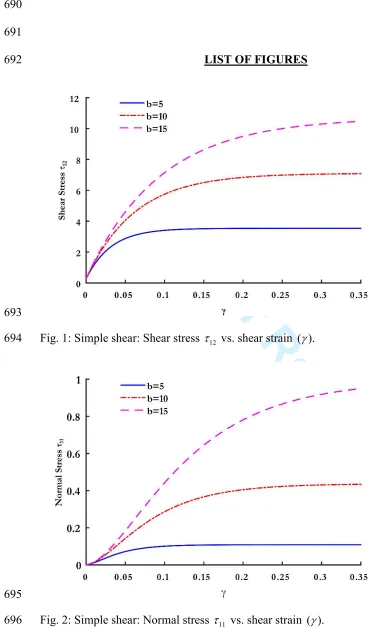
₁₂ and the normal

τ

₁₁stress 471

components, respectively. By referring to Fig.1, we observe that the model predicts 472

continuous stress-deformation curves, with a non-unambiguously specified elastic portion

473

and a non-well defined yield stress, which as the deformation increases converge to a

474

(constant) stress which may be defined as the material ultimate strength; we note that the 475

higher the value of ,

β

the higher is the predicted ultimate strength. Such a response is in 476

absolute accordance with the one exhibited by almost all advanced metallic alloys; 477

compare for instance the predicted behavior with the ones reported by Chen et al. in [8]. 478

479

480

5.2 Tension-compression tests

481

482

As a second example we discuss the predictions of the model for some tension-483

compression tests. These tests, in general, are defined as 484

1 _{(1 )} 1_, 2 _{(1 )} 2_, 3 _{(1 )} 3_,

x = +

χ

X x = +

ψ

X x = +

ψ

X

485

where 1+

χ

( )t and 1+

ψ

( )t are the principal stretches along the longitudinal and the 486

transverse directions respectively. By means of this example we’ll demonstrate the ability 487

of the model in predicting several patterns of the real response of metals which cannot be 488

For Peer Review

As a first simulation we consider a loading history comprising loading-unloading-490

reloading. The results for two different values of the parameter R and a constant value of 491

( =5),

β β

are shown in Fig. 3. In this case we verify the ability of the model to predict 492

the real response of metals - recall section 3 - according to which, the reloading, 493

following (plastic) loading and subsequent (elastic) unloading, results at plastic 494

deformation at any stress level. Moreover, depending on the value of R, the reloading 495

curve may or may not converge (asymptotically) to the monotonic loading curve. The 496

later pattern of response corresponds to the so-called long-term or permanent softening

497

effect (see, e.g., [39,37]), which plays an important role in the numerical simulation and

498

design of metal sheets in forming processes. This phenomenon appears alike in a (two-499

sided) tension-compression test (see Fig. 4). 500

As a second simulation we study the (low cycle) fatigue behavior at low stress levels 501

(see Fig. 5). For this purpose we perform a loading-unloading-reloading test at a small 502

stress level, by selecting a value for R (R=30), such as the reloading curve convergences 503

to the corresponding loading curve. Next, we perform a loading-unloading test, but now 504

the specimen is subjected to a cyclic loading with stress amplitude equal to the stress 505

level where the (first) unloading began. Upon referring to the results of Fig. 5, we note 506

the ability of the model in predicting (real) material behavior, which consists of the 507

appearance of residual strains - apparently plastic - and accumulation of plastic work. 508

Moreover, due to the material fatigue, permanent softening phenomena appear in a rather 509

For Peer Review

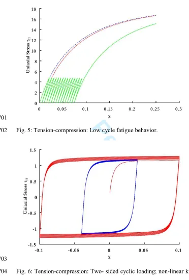
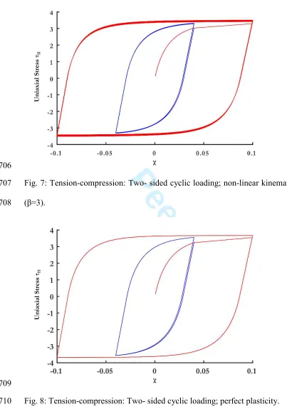
As a final simulation, we consider the case where the material is subjected to (two-511

sided) cyclic loading. For this problem we consider that the kinematic hardening law (27) 512

may be replaced by the standard (non-linear) Armstrong-Frederic hardening law, i.e. 513

2

= ,

3

L_va HL_vb_e−La

κ

&

514

where L is the non-linear (kinematic) hardening modulus. The remaining model 515

parameters are set equal to 516

300.00, =0.3, R=30.00, 0.10, 0.3, 30.

E=

ν

K = H = L=

517

The results of this test, for two different values of the parameter

β

are shown in Figs. 6 518

and 7. The model predicts stresses which are increasing as the number of cycles increases 519

and eventually stabilize at a constant value after a few cycles. This response constitutes 520

the very essence of the cyclic behavior of mild steels (see, e.g., Fig. 6a in [39]). The 521

predictions of the model in the absence of hardening mechanisms (K =H = =L 0) are 522

also presented in Fig. 8 ( =3).

β

In this case, the model has the ability to predict almost 523

stabilized stress-deformation curves from the first cyclic of strain. This response is 524

identical to the one exhibited by dual-phase high strength steel specimens (see, e.g., 525

figure 6b in [39]) 526

527

528

6. Concluding remarks

529

530

The basic impact of this paper relies crucially in providing deeper insights into the 531

For Peer Review

i. Motivated by a question posed in a very recent paper by Xiao et al. [37], we 533

have shown how the basic concepts in plasticity theory can be introduced in a 534

purely mathematical manner, upon studying the properties of a suitably 535

formulated differential equation and involving the basic concepts of loading and 536

unloading. The proposed formulation is rather general and includes classical 537

plasticity as a special case. 538

ii. We have revisited the quasi-yield surface concept by clarifying some basic 539

theoretical issues related to it. 540

iii. We have shown how the concept can be applied in the constitutive modeling of 541

solid materials and in particular in metals, upon developing a rather simple 542

material model. 543

Moreover, we have implemented the model numerically and we have demonstrated its 544

ability in predicting several patterns of the complex response of metals which cannot be 545

predicted by the conventional plasticity models. 546

547

548

References

549

[1] R. Abraham, J. E. Marsden and T. Ratiu. Manifolds, tensor analysis and 550

applications, 2nd edition. Springer-Verlag, New York Inc. (1988). 551

552

[2] S. N. Atluri. On the constitutive relations at finite strain. Hypo-elasticity and elasto- 553

plasity with isotropic or kinematic hardening. Computer Methods Appl. Mech. Engrg. 554

43, 137-171 (1984). 555

556

[3] J. E. Bell. The Experimental Foundations of Solid Mechanics. In: Handbuch der 557

Physik, BandVIa/1, ed. C. Trusesdell, Springer, Berlin (1973). 558

559

[4] A. Bertram. An alternative approach to finite plasticity based on material 560

For Peer Review

562

[5] A. Bertram and M. Kraska. Description of finite plastic deformations in single 563

crystals by material isomorphisms. In: Proceedings of IUTAM & ISIMM Symposium 564

on “Anisotropy, Inhomogeneity and Nonlinearity in Solid Mechanics”, 30.8.-3.9.94 565

Nottingham, eds. D. F. Parker, A. H. England, KLUWER Academic Publ. 39, 77-90 566

(1995). 567

568

[6] S. S. Bodner. Constitutive equations for dynamic material behavior. In: Mechanical 569

Behavior of Materials under Dynamic Loads, Symp. San Antonio, ed. U. S. Lidholm, 570

Springer-Verlag, New York 176-190 (1968). 571

572

[7] S. R. Bodner and Y. Partom. Constitutive equations for elastic-viscoplastic strain 573

hardening materials. J. Appl. Mech. 39, 385-389 (1975). 574

575

[8] Z. Chen, H. J. Bong, D. Li and R. H. Wagoner. The elastic–plastic transition of 576

metals. Int. J. Plast. 83, 178-201 (2016). 577

578

[9] A. F. Cheviakov, J. F. Ganghoffer and R. Rahouadj. Finite strain plasticity models 579

revealed by symmetries and integrating factors: The case of Dafalias spin model. Int. 580

J. Plast. 44, 47-67 (2013). 581

582

[10] M. A. Eisenberg and A. Phillips. A theory of plasticity with non-coincident yield and 583

loading surfaces. Acta Mech. 11, 247-260 (1971). 584

585

[11] M. Hollenstein, M. Jabareen and M. B. Rubin. Modeling a smooth elastic-inelastic 586

transition with a strongly objective numerical integrator needing no iteration. Comp. 587

Mech. 52, 649-667 (2013). 588

589

[12] M. Jabareen. Strongly objective numerical implementation and generalization of a 590

unified large inelastic deformation model with a smooth elastic-inelastic transition. 591

Int. J. Eng. Sci. 96 46-67 (2015) 592

593

[13] E. Kroner and C. Theodosiu. Lattice defect approach to plasticity and viscoplasticity. 594

In: Problems of Plasticity, ed. A. Swaczuk, Noordoff, Leyden, 45-88 (1972). 595

596

[14] E. H. Lee. Elastic-plastic deformations at finite strains. J. Appl. Mech. 36, 1-6 597

(1969). 598

599

[15] C.-S. Liu and H.-K.Hong. Using comparison theorems to compare corrotational rates 600

in the model of perfect elastoplasticity. Int. J. Solids Struct. 38, 2969-2987 (2001). 601

602

[16] J. Lubliner. On the structure of the rate equations of material with internal variables. 603

Acta Mech. 17, 109–119 (1973). 604

605

[17] J. Lubliner. A simple theory of plasticity. Int. J. Solids Struct. 10: 313-319 (1974). 606

For Peer Review

[18] J. Lubliner. On loading, yield and quasi-yield surfaces in plasticity theory. Int. J. 608

Solids Struct. 11: 1011-1016 (1975). 609

610

[19] J. Lubliner. An axiomatic model of rate-independent plasticity. Int. J. Solids Struct. 611

16: 709-713 (1980). 612

613

[20] J. Lubliner. A maximum-dissipation principle in generalized plasticity Acta 614

Mech. 52: 225-237 (1984). 615

616

[21] J. Lubliner. Plasticity Theory. Macmillan, New York (1990). 617

618

[22] J. Lubliner. A simple model of generalized plasticity Int J. Solids Struct. 28: 769- 619

778 (1991). 620

621

[23] J. Lubliner, R. L. Taylor and F. Auricchio. A new model of generalized plasticity 622

and its numerical implementation. Int J. Solids Struct. 30: 3171-3184 (1993). 623

624

[24] M. Lucchesi and P. Podio-Guidugli. Materials with elastic range: a theory with a 625

view toward applications. Part II. Arch. Rat. Mech. Anal. 110, 9-42 (1992). 626

627

[25] J. Mandel. Plasticite′classique et viscoplasticite .′ Courses and Lectures, No 97. 628

International Center for Mechanical Sciences, Udine, Springer, New York (1971). 629

630

[26] V. P. Panoskaltsis VP, L. C. Polymenakos and D. Soldatos. Eulerian structure of 631

generalized plasticity: Theoretical and Computational Aspects. J. Engng. Mech. 632

ASCE 134, 354-361 (2008). 633

634

[27] V. P. Panoskaltsis, D. Soldatos and S. P. Triantafyllou. The concept of physical 635

metric in rate-independent generalized plasticity. Acta Mech. 221, 49-64 (2011). 636

637

[28] V. P. Panoskaltsis VP, L. C. Polymenakos and D. Soldatos. A finite strain model 638

of combined viscoplasticity and rate-independent plasticity without a yield surface. 639

Acta Mech. 224, 2107-2125 (2013). 640

641

[29] V. P. Panoskaltsis and D. Soldatos. A phenomenological constitutive model of non 642

-conventional elastic response. Int. J. Appl. Mech. 5 DOI: 643

10.1142/S1758825113500361 (2013). 644

645

[30] A. C. Pipkin and R. S. Rivlin. Mechanics of rate-independent materials. Z. Angew. 646

Math. Phys. 16, 313-327 (1965). 647

648

[31] M. B. Rubin. An elastic-viscoplastic model for large deformation. Int. J. Engng. 649

Sci., 24, 1083-1095 (1986). 650

651

[32] M. B. Rubin. An elastic-viscoplastic model exhibiting continuity of solid and fluid 652

For Peer Review

654

[33] J. C. Simo. A framework for finite strain elastoplasticity based on maximum plastic 655

dissipation and the multiplicative decomposition: Part I. Continuum Formulation. 656

Computer Methods Appl. Mech. Engrg. 66, 199-219 (1988). 657

658

[34] J. C. Simo and T. J. R. Hughes. Computational inelasticity. Springer-Verlag New 659

York, Inc. (1997). 660

661

[35] D. Soldatos and S. P. Triantafyllou. Logarithmic spin, Logarithmic rate and material 662

frame-indifferent generalized plasticity. Int. J. Appl. Mech. 08, 1650060 (2016). 663

664

[36] H. Stumpf and U. Hoppe. The application of tensor algebra on manifolds to non- 665

linear continuum mechanics. Invited survey article. Z. Angew. Math. Mech. 77, 327- 666

339 (1997). 667

668

[37] L. Sun and R. H. Wagoner. Proportional and non-proportional hardening behavior 669

of dual-phase steels. Int. J. Plast. 45, 174-187 (2013). 670

671

[38] H. Xiao, O. T. Bruhns and A. Meyers. Free rate-independent elastoplastic equations. 672

Z. Angew. Math. Mech. 94, 461-476 (2014). 673

674

[39] F. Yoshida, T. Uemori and K. Fujiwara. Elastic-plastic behavior of sheet steels under 675

in-plane cyclic tension-compression at large strain. Int. J. Plast. 18, 633-659 (2002). 676

677

[40] Kubo, R., Some aspects of the statistical-mechanical theory of irreversible processes. 678

Lectures in theoretical physics, 1, pp.120-203 (1959). 679

680

681

682

683

684

685

686

687

688

For Peer Review

690

691

LIST OF FIGURES

692

[image:31.612.50.426.75.711.2]

693

Fig. 1: Simple shear: Shear stress

τ

₁₂ vs. shear strain ( ).γ 694

695

For Peer Review

697

Fig. 3: Tension-compression: Loading-unloading-reloading (one-sided). 698

699

For Peer Review

[image:33.612.58.430.73.624.2]

701

Fig. 5: Tension-compression: Low cycle fatigue behavior.

702

[image:33.612.103.419.87.317.2]

703

Fig. 6: Tension-compression: Two- sided cyclic loading; non-linear kinematic hardening 704

For Peer Review

706

Fig. 7: Tension-compression: Two- sided cyclic loading; non-linear kinematic hardening 707

(β=3). 708

[image:34.612.56.459.73.643.2]

709