Author’s Accepted Manuscript
EPRENNID: An evolutionary prototype reduction
based ensemble for nearest neighbor classification
of imbalanced data
Sarah Vluymans, Isaac Triguero, Chris Cornelis,
Yvan Saeys
PII:
S0925-2312(16)30866-9
DOI:
http://dx.doi.org/10.1016/j.neucom.2016.08.026
Reference:
NEUCOM17437
To appear in:
Neurocomputing
Received date: 27 November 2015
Revised date:
7 July 2016
Accepted date: 4 August 2016
Cite this article as: Sarah Vluymans, Isaac Triguero, Chris Cornelis and Yvan
Saeys, EPRENNID: An evolutionary prototype reduction based ensemble for
nearest
neighbor
classification
of
imbalanced
data,
Neurocomputing,
http://dx.doi.org/10.1016/j.neucom.2016.08.026
This is a PDF file of an unedited manuscript that has been accepted for
publication. As a service to our customers we are providing this early version of
the manuscript. The manuscript will undergo copyediting, typesetting, and
review of the resulting galley proof before it is published in its final citable form.
Please note that during the production process errors may be discovered which
could affect the content, and all legal disclaimers that apply to the journal pertain.
EPRENNID: An Evolutionary Prototype Reduction
Based Ensemble for Nearest Neighbor Classification of
Imbalanced Data
Sarah Vluymansa,b,c,∗, Isaac Triguerob,d,e, Chris Cornelisa,c, Yvan Saeysb,d
aDepartment of Applied Mathematics, Computer Science and Statistics, Ghent
University, Belgium
bVIB Inflammation Research Center, Ghent, Belgium
cDepartment of Computer Science and Artificial Intelligence, University of Granada,
Spain
dDepartment of Internal Medicine, Ghent University, Belgium
eSchool of Computer Science, University of Nottingham, Jubilee Campus, Wollaton
Road, Nottingham NG8 1BB, United Kingdom
Abstract
Classification problems with an imbalanced class distribution have received an increased amount of attention within the machine learning community over the last decade. They are encountered in a growing number of real-world situations and pose a challenge to standard machine learning tech-niques. We propose a new hybrid method specifically tailored to handle class imbalance, called EPRENNID. It performs an evolutionary prototype reduction focused on providing diverse solutions to prevent the method from overfitting the training set. It also allows us to explicitly reduce the under-represented class, which the most common preprocessing solutions handling class imbalance usually protect. As part of the experimental study, we show that the proposed prototype reduction method outperforms state-of-the-art preprocessing techniques. The preprocessing step yields multiple prototype sets that are later used in an ensemble, performing a weighted voting scheme with the nearest neighbor classifier. EPRENNID is experimentally shown to significantly outperform previous proposals.
Keywords: Imbalanced data, Prototype selection, Prototype generation,
∗Corresponding author
Differential evolution, Nearest neighbor
1. Introduction
Class imbalance is present in a dataset when its instances are unevenly distributed among the classes. It is encountered in many real-world situations such as medical diagnosis [1], microarray data analysis [2] or software quality evaluation [3]. Many applications are inherently prone to class imbalance, motivating the increased amount of attention to this issue within the machine learning community [4].
The class imbalance problem [5] refers to the fact that the performance of learning algorithms can be severely hampered by data imbalance. In this work, we focus on two-class imbalanced classification, where the elements of the majority class outnumber those of the minority class. Traditionally, the majority elements are denoted as negative, whereas the minority ele-ments are referred to as positive. Standard classification techniques may not perform well in this context, as they internally assume equal class distribu-tions. Consequently, over the last decade, a considerable amount of work has been proposed in the specialized literature to alleviate the imbalance prob-lem [6, 7, 8]. Some approaches work at the data level, while others develop custom classification processes. At the data level, the so-called data sampling methods modify the training dataset to produce a better balance between classes [9, 10]. Solutions at the algorithm level are modifications of exist-ing methods and internally deal with the intrinsic challenges of imbalanced classification [11, 12].
best of our knowledge, no hybrid PS-PG techniques have been developed to deal with imbalanced classification problems so far.
In this paper, we propose a combined model for the classification of two-class imbalanced data, integrating both a hybrid preprocessing and a two- classifi-cation step. We extend the framework of [23] for use in the presence of class imbalance, considerably modifying both PS and PG stages. We also aim at introducing diversity in the process. The multiple prototype sets resulting from the preprocessing step are further combined in a custom ensemble for classification. The classification step is an extension of the k nearest neigh-bor classifier (kNN, [24]). We call our method EPRENNID, an Evolutionary Prototype Reduction based Ensemble for Nearest Neighbor classification of Imbalanced Data.
The main contributions of this work are as follows:
• We first introduce a new evolutionary PS method specifically tuned to handle class imbalance. Although it is related to undersampling meth-ods, it takes a step away from them by allowing the removal of minority elements from the dataset, as in [25]. Most existing methods do not allow such kind of reduction of non-representative or noisy elements from the positive class.
• To alleviate the overfitting issues of prototype reduction models, we take advantage of the evolutionary nature of the proposed method. Instead of yielding a single reduced set, EPRENNID provides several well-performing and diverse ones.
• The evolutionary PG method used in this work [23] has been modified to handle the class imbalance problem.
• Finally, the optimized prototype sets are used in a classifier ensemble, using an adaptive scheme selecting the most suitable prototype sets to classify each single target instance with kNN.
The remainder of this paper is structured as follows. In Section 2, we review the PS and PG schemes and provide more details on related work in imbalanced classification. Section 3 introduces the proposed model, with a detailed explanation of the separate preprocessing and classification phases. We have conducted a comprehensive experimental study. Its setup is de-scribed in Section 4, while Section 5 lists and discusses our results. Finally, Section 6 formulates the conclusions of this work and outlines future research directions.
2. Preliminaries and related work
This section provides the necessary background for the remainder of the paper. Sections 2.1 presents prototype selection and generation techniques, focusing on the methods on which our model is based. Section 2.2 introduces the problem of classification with imbalanced datasets and its evaluation is recalled in Section 2.3.
2.1. Prototype reduction
Prototype reduction techniques aim to reduce the available training set
T ={x1, x2, . . . , xn} of labeled instances to a smaller set of prototypes S =
{y1, y2, . . . , yr}, with r < n and each yi either drawn from T or artificially
constructed. The set S, rather than the entire set T, is used afterwards to train the classifier.
These methods are commonly combined and designed to be used with the
kNN classifier. This lazy learning algorithm [26] assigns new input instances to the class to which the majority of theirk nearest neighbors in the training set belongs. Despite its performance, it suffers from several drawbacks such as low efficiency, high storage requirements and sensitivity to noise. PS and PG techniques can be beneficial to alleviate these issues. To that end, the instances contained in S should form a good representation of the original class distributions. Furthermore, their size relative to that of T should be small enough in order to considerably reduce the storage and execution time requirements of kNN.
A PS method reduces T to S by selecting a subset of its instances. This implies that for every instance yi ∈ S there exists an element xj ∈ T such
that yi = xj. In [19], a taxonomy for PS methods was proposed and an
artificial ones, while the latter is restricted to selecting elements from T. Therefore, a set S constructed by a PG method is not necessarily a subset of
T, allowing for a larger flexibility in the construction ofS. For PG methods, a related taxonomy has been proposed in [20]. In what follows, we describe the PS and PG methods on which we base our proposal.
2.1.1. Steady State Memetic Algorithm for Instance Selection
The Steady State Memetic Algorithm (SSMA) is a genetic algorithm for PS. In several experimental studies (e.g. [19, 23]), it has been shown to be one of the best-performing PS methods, which is due to its optimization procedure performed in each iteration. As a genetic algorithm, it evolves a population of I individuals, the chromosomes, over a number of generations
G. Each individual corresponds to a candidate subset and is encoded as a bitstring, where a 0 in the ith position means that the ith element of T
is not included in the subset, while a 1 means that it is. The quality of an individual, that is, how good a solution it is, is evaluated by a so-called fitness function. To calculate the fitness of a candidate subset S, SSMA uses a combined criterion, namely the accuracy of thekNN classifier on the entire training setT usingS as prototype set and the reduction in size ofS relative to T.
The population is optimized over the subsequent generations, such that the final fittest individual corresponds to an optimal solution. To guide the evolution, it uses two genetic operators: crossover and mutation. In each generation, two parents are selected to produce two new individuals by means of the Half Uniform Crossover (HUX) procedure: positions in which the parents take on the same value, are simply copied to the children, while for the remaining ones, each child randomly copies half of each parent.
2.1.2. Scale Factor Local Search in Differential Evolution
Scale Factor Local Search in Differential Evolution (SFLSDE) [28] was shown to be one of the top performing PG methods in the experimental study of [23]. It is a positioning adjustment algorithm, optimizing the positions of the instances in the dataset. The method uses differential evolution (DE, [29, 22]), which follows the evolutionary framework, evolving a population of candidate solutions over a number of generations. The evolution is guided by custom mutation and crossover operators. In general, for each individ-ual xi, mutation is achieved by randomly selecting two other chromosomes
x1 and x2 from the current population. A new individual is created by
in-creasing xi by the difference of x1 and x2, weighted by a scale factor F >0.
A number of different mutation operators exist, but we have chosen to use the DE/RandToBest/1 strategy, which makes use of the current fittest xbest
individual in the population. It increases xi by both the difference of the
two randomly selected individuals as well as the difference of xi and xbest,
weighting both terms by F. After mutation, crossover is performed, ran-domly modifying the mutated individual in certain positions. The crossover is guided by another user-specified parameter Cr.
SFLSDE is a memetic DE algorithm and modifies the general mutation and crossover schemes, integrating two local searches. The method uses adaptive values for the F and Cr parameters. Specifically, each instance xi
has its custom values Fi and Cri values assigned to it, which are updated in
each iteration. When updating the scale factors Fi, two local searches are
used: the golden section search and hill-climbing. We refer to [28] for further details.
2.2. Imbalanced classification
In a wide range of classification problems, the number of instances that belong to each class can be radically skewed. Standard classifiers tend to be biased towards the majority class, although the minority class is normally the most interesting class.
done in a random way [9] or more complex heuristics for selecting majority class candidates for removal can be put in place [30, 16]. By reducing the size of the dataset, undersampling methods are actually performing proto-type selection. However, they are constrained in their application, as they are usually only allowed to reduce the majority class, leaving the minority elements untouched.
The strategy adopted by a second kind of methods consists of finding a more favorable balance between classes by means ofoversampling the minor-ity class. The size of this class is increased by adding duplicates of existing minority instances or by constructing artificial elements based on the ones at hand. A straightforward approach is presented in [9]. It involves the du-plication of randomly selected minority elements. The SMOTE technique [10] laid the foundation of more complex oversampling methods. Instead of duplicating existing minority elements and thereby increasing their weight in the dataset, it generates a number of synthetic instances assigning them to the minority class. Several later proposals (e.g. [31, 32, 33]) are modifica-tions of SMOTE, replacing some of its random components by more complex procedures.
Finally, several hybrid data sampling methods, both undersampling the majority and oversampling the minority class, have been designed as well. They often combine an initial oversampling step by posterior data cleaning [9]. The first phase usually results in a perfectly balanced dataset, on which the data cleaning is executed. The latter can be performed on either the entire intermediate set or be restricted to the newly generated instances. Alternatively, a complete intertwining of the oversampling and undersam-pling approaches can be set up, generating minority elements and removing majority instances at the same time [34, 35].
Apart from the data level approaches discussed above, some specific clas-sification algorithms tolerating class imbalance have been proposed as well. These include the cost-sensitive learners, like cost-sensitive kNN [12], cost-sensitive C4.5 [11], cost-cost-sensitive SVM [36, 37] and cost-cost-sensitive neural net-works [38], which modify traditional classifiers by assigning different costs to the misclassification of minority and majority instances. These costs are used in the construction of the classification model and reduce the dominance of majority over minority elements.
such as the boosting [40] or bagging [41] schemes, and incorporate some heuristics to deal with class imbalance or cost-sensitive models [42]. Other ensemble-based approaches analyze the influence of noisy data in imbalanced classification [43]. Prominent and recent examples include the SMOTEBoost [44], SMOTEBagging [45], RB-Bagging [46], NBBag [47], and EUSBoost [48] methods. Very recent proposals also deal with multi-class imbalanced data [49].
2.3. Evaluation of imbalanced classifiers
In this section, we review the important issue of the evaluation of the classification performance on imbalanced data. Table 1 presents a generic confusion matrix for binary classification problems, displaying the number of true positives (TP), true negatives (TN), false positives (FP) and false negatives (FN) obtained in a classification experiment. As this paper focuses on binary problems, we restrict this matrix to the binary case as well, but its generalization to more than two classes is straightforward.
Table 1: Confusion matrix obtained after classification of a two-class dataset
Actual/Predicted Positive Negative
Positive TP FN
Negative FP TN
In traditional classification applications, the performance of a classifier is commonly assessed by the classification accuracy (percentage of correctly classified examples, that is, acc= T P+T Nn , wherenis the size of the dataset). In the presence of class imbalance this measure usually provides misleading results, because it does not distinguish between the number of correct labels of different classes, making it sensitive to skewness in class distributions [50]. As an alternative to the overall accuracy, the geometric mean g meanis often used [16, 51, 52]. This measure is defined as
g mean=
r
T P T P +F N ·
T N T N+F P.
classifiers on binary problems and reflects the trade-off between its true pos-itive T P and false positive F P rates. The area under it expresses how well the classifier achieves this, in a single measure.
For a discrete classifier, outputting actual class labels rather than class probability estimates, a ROC-curve can be constructed by converting its crisp output to the required class probabilities. As noted in [53], one needs to consider the inner workings of the method to extract these values. For example, when applying the kNN classifier on a binary problem, an instance is assigned to the class to which the majority of its k nearest neighbors belong. The probabilities of belonging to the positive and negative classes can be set to k+
k and k−
k respectively, where k+ represents the number of
positive elements among the k neighbors and k− the number of negative
ones. As shown in [54], when k = 1, the AUC is computed as
AU C = 1 +T P −F N
2 .
The difference between AUC and g mean is that the AUC presents a global picture of the strength of the classifier, varying the threshold of how likely instances should belong to the positive class to be assigned to it (except in the case of kNN and k = 1), while g mean solely considers the standard decision criterion, assigning instances to the class to which they most likely belong.
As discussed in [53], ROC-curves are insensitive to changes in class dis-tribution, rendering the AUC a proper measure to use in the classification of imbalanced data. This results from the fact that the points of the curve are determined using the row-wise ratios of the confusion matrix. By using the rows separately, the ROC-curve and the AUC do not depend on the actual class distribution.
3. Proposed model: EPRENNID
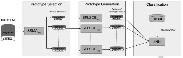
In this section, we introduce our new model for the classification of im-balanced data, incorporating both a preprocessing and a classification step. The former involves the combination of PS and PG and the latter uses an en-semble of well-performing prototype sets, provided by the preprocessing step, in a weighted voting scheme. Its different stages are depicted in Figure 1.
Figure 1: Schematic workflow of EPRENNID. In a first step, diverse prototype sets (numP S) are selected from the training data using the proposed SSMAImb algorithm.
These prototype sets are refined by using SFLSDEImb to optimize the positioning of the
prototypes of every subset. Finally, the resulting pre-processed datasets are used in a weighted vote to classify test instances.
with the classification part of our model, which is an ensemble approach using kNN.
3.1. Preprocessing: a hybrid prototype reduction model for imbalanced data
In this section, we propose a hybrid prototype reduction model to pre-process imbalanced data. Based on the model presented in [23], in which the authors combined PS and PG models for standard classification, our proposal will hybridize these two processes to alleviate the weaknesses of the isolated models in the imbalanced context.
By means of PS, a number of well-performing prototype sets are gen-erated, which are further optimized using a PG method. The underlying motivation for applying such hybridization is that PG models are more flexi-ble than PS techniques, allowing us to obtain more accurate reduced sets that are not limited to selecting a subset of instances from the original training set. However, PG models also suffer from several drawbacks such as initial-ization issues (appropriate choice of the number of prototypes per class) and more complex search spaces, in which PS models can be exploited to ease the posterior PG process. More details about the benefits of hybridizing PS and PG can be found in [23]. We use the most successful combination sug-gested by their experiments: the PS method SSMA (Section 2.1.1) and the PG method SFLSDE (Section 2.1.2).
[image:11.612.115.504.124.248.2]problems of these models and handle imbalance problems.
• Firstly, we provide a wide variety of reduced sets with a newly proposed PS method, SSMAImb. This method entirely replaces the SSMA step
in [23] to take into account the class imbalance, allowing elimination of both positive and negative examples (Section 3.1.1).
• Secondly, the optimization performed by SFLSDE has been modified as well (named SFLSDEImb), by means of a new objective function,
more appropriately evaluating the performance of a prototype set in a classification process (Section 3.1.2).
• Finally, we combine the above two methods in a hybrid setting, opti-mizing multiple SSMAImb generated prototype sets with SFLSDEImb.
We use a diversity mechanism to select a diverse set of well-performing prototype sets to deal with the overfitting problem often encountered by PG. They are later optimized in separate populations, out of which a final diverse set is again selected to be used in the classification step. In this way, during classification, EPRENNID has the flexibility to select prototype sets that have proven to perform well in the neighborhood of a specific target, instead of relying on one prototype set to perform well in the entire feature space (Section 3.1.3).
3.1.1. SSMAImb
Even though SSMA performs very well on balanced data, it fails when faced with class imbalance. A preliminary experimental study [54] showed that the direct application of this method significantly worsens the classifi-cation performance and tends to remove all the examples from the minority class. Nevertheless, its good performance on balanced data, its use of the optimization step and its flexibility motivated us to adapt it to tackle imbal-anced problems. We have kept the defining aspects of SSMA in place, i.e. it remains a steady state memetic algorithm, but we have integrated some imbalance-resistant heuristics at three crucial points: the fitness function, the parent selection mechanism and the meme optimization. We call the modified method SSMAImb.
Fitness function modifications
evaluating the classification performance by the accuracy and explicitly using the reduction, small subsets consisting of mostly negative elements can easily attain high fitness values and give the impression of representing high quality subsets. As an example, consider a training set T consisting of 10 positive and 90 negative elements and a singleton candidate subsetS of one negative instance. Using the 1NN rule as the classifier, all instances are classified as negative, yielding an accuracy of 90%. The reduction rate would be 99%. The combination results in a high fitness value, even though this set will never be able to classify any positive element correctly. To remedy this situation, we propose a new fitness function, similar to the one used in [16]:
f itness(S) = g mean−
1− 1
IRS
·P, (1)
where g mean replaces the accuracy to evaluate the classification perfor-mance of S. This is determined by using kNN and leave-one-out cross-validation. The value IRS corresponds to the imbalance ratio of the set S.
This measure evaluates how imbalanced a set is and is defined as IRS = M ajM inSS,
whereM ajS andM inScorrespond to the cardinality of the majority and
mi-nority classes inS respectively. It is important to note that the majority and minority classes in S do not necessarily correspond to those in T. Finally, the parameterP determines the weight of the second term and therefore how much class imbalance is penalized in S. The authors of [16] proposed to use
P = 0.2 and we have adopted this value as well. We evaluated other values for P in a preliminary experimental study, but no significant differences in performance were observed, so we decided to use its default value. The new fitness function favors subsets S with a good classification performance and that are not too imbalanced. The fitness function is used to decide whether the meme optimization is applied or not. In a later stage of our proposal (see Section 3.1.3), it is also applied in the selection of the fittest individuals.
Parent selection mechanism
When selecting parents to create offspring, the original SSMA method assigns a higher probability of being selected to individuals with a higher fitness. However, SSMAImbdoes not use the fitness measure for such purpose,
because it is more focused on providing good classification performance (P = 0.2). The parent selection procedure of SSMAImb aims to explicitly favor
while keeping the g-mean high, independently of any parameterP. Thus, we propose a new measure, defined as
Sel(S) = 2· g mean·
1 IRS
g mean+ IR1
S
, (2)
which corresponds to the harmonic mean of g meanand IR1
S. The harmonic
mean of two values tends more strongly to the smaller one, meaning that both inputs should attain high values for it to be large. In this case, this corresponds to a high value for g meanand low IR. Chromosomes attaining higherSel(·) values have a higher probability of being selected for reproduc-tion.
The HUX operator must deal with a constraint posed by imbalanced problems: avoid creating children that do not contain any positive instances. For example, consider two parents that differ in all genes in a dataset with
|T|= 11, with 3 positive and 8 negative instances: 1 0 1
| {z }
M inority
0 1 0 1 0 1 0 1
| {z }
M ajority
and 0 1 0
| {z }
M inority
1 0 1 0 1 0 1 0
| {z }
M ajority
.
In the construction of their children, randomly half of the positions of each parent are used. This could yield a child without minority class elements:
0 0 0
| {z }
M inority
1 0 1 1 0 1 0 1
| {z }
M ajority
.
To tackle this issue, the HUX operator will be initially limited to the positions of the majority elements. This creates two partial children with only majority elements. Next, the minority positions are filled up in each child. When both parents take on the same value, this value is copied to the child. Otherwise, we set the position to 1 while there are fewer minority than majority elements in the chromosome. When a perfect balance has been achieved, we go back to selecting a random value. This procedure depends on the order in which the minority genes are considered. We first use the genes set to 1 in the fittest parent, randomly ordered.
Meme optimization
g mean measure, while we now evaluate classification performance by the AUC. By incorporating the two measures in the PS algorithm, we avoid over-fitting one of them and instead aim to optimize both. Furthermore, instead of trying to increase the reduction, we are allowing only majority positions to be set to 0 and minority positions to be set to 1. The majority and minor-ity classes are again determined within the chromosome at hand. When the chromosome is perfectly balanced, that is, the same number of elements for both classes are selected, no optimization is performed. Note that an empty set S is also perfectly balanced, but in such a situation S is optimized by adding an arbitrary element of each class. By setting majority genes to 0 and minority genes to 1, IRS can only decrease, possibly up to a point where
a perfect balance is achieved and an imbalance in the other direction would be created. To prevent this, the optimization halts prematurely when this occurs. We present the modified optimization procedure in Algorithm 1.
Algorithm 1 Optimization procedure of SSMAImb
Require: A chromosomeS={s1, s2, . . . , sn}
Ensure: The optimized chromosome
1: Determine the majority and minority class inS.
2: whilethere are untested positionsdo
3: S∗←S.
4: Select a random untested minority position withsi = 0 or majority position with
si= 1.
5: Change the value of the selected position inS∗.
6: AU CS∗ ←AUC ofkNN, usingS∗ as prototype set.
7: AU CS ←AUC ofkNN, usingS as prototype set.
8: gain←AU CS∗−AU CS.
9: if gain≥µthen
10: S←S∗
11: end if
12: if IRS = 1then
13: halt the optimization
14: end if
15: end while
0.001. When the reduction corresponding to the best chromosome has not increased for a given number of populations, µ is decreased by 0.001. The value 0.001 was chosen as it is used in combination with the AUC, which is a number in the interval [0,1].
3.1.2. SFLSDEImb
As a second step in the preprocessing phase, we apply a PG algorithm. We have opted to combine SSMAImb with a modified version of SFLSDE.
This combination yielded the best results in [23], making it a potential can-didate for extension to imbalanced classification problems. Nevertheless, the authors used the accuracy of the 1NN classifier to evaluate the fitness of the individuals during DE. Following our discussion in Section 2.3, the ac-curacy is not an appropriate fit performance measure for class imbalance in the training set and we have accordingly changed it to g mean. We do not modify the other DE operators of mutation and crossover as we did in the PS step. The PG method is applied after the dataset has been preprocessed by SSMAImb. The individuals coming from this PS step are already more
balanced, implying that the genetic operators in SFLSDE do not have to be specifically tuned to handle class imbalance. As before, we denote the modified DE algorithm as SFLSDEImb.
3.1.3. Hybridizing SSMAImb and SFLSDEImb
As SSMAImb is a genetic algorithm, it encounters a high number of
can-didate prototype sets during its run. Even though these do not correspond to the final fittest solution, they might still constitute valid alternatives per-forming well in the classification. To use these solutions and enhance the performance of our algorithm, we therefore do not restrict ourselves to se-lecting only the fittest solution found by SSMAImb, but rather select a diverse
set of fit individuals, setting up a voting committee for the final classification step (Section 3.2).
The user specifies the desired number numP S of prototype sets, which are selected from among the 50% fittest chromosomes encountered during the entire execution. The selection procedure is described in Algorithm 2. The first set is chosen as the overall fittest one. The remaining sets are selected by an incremental procedure, continuously adding subsets diverse enough from the ones previously selected, until numP S have been chosen.
The diversity measure between two prototype sets S1 and S2 is based
community that ensures a good level of diversity in the classification behavior of two datasets [56]. It has recently been shown that promoting diversity by means of the Q-statistic in an ensemble for imbalanced classification has a positive effect on its performance evaluated by both AUC and g mean [57]. The examples of the training set T are classified with the 1N N rule, using both prototype sets S1 and S2 as reference sets. Their diversity is computed
as follows:
diversity(S1, S2)←1−
n00n11−n01n10
n00n11+n01n10
, (3)
where n00 represents the number of instances that none of the classifiers
predicted correctly,n11 the number of samples correctly classified by both of
them, and n01 and n10 counts the number of samples predicted by S1 and
not by S2 and vice versa.
Algorithm 2 Selection of a diverse set of fit prototype sets
Require: A complete setSof candidate prototype sets, an integernumP S
Ensure: Setdiv ofnumP S selected prototype sets
1: div← {S}, whereS is the fittest individual inS
2: numP S←numP S−1 3: whilenumP S >0 do
4: diversitymax←0
5: Sbest←null
6: for allS∈S do
7: diversitycurr←0 8: for allP ∈div do
9: diversitycurr←diversitycurr+diversity(S, P)
10: end for
11: if diversitycurr> diversitymaxthen 12: diversitymax←diversitycurr
13: Sbest←S
14: end if
15: end for
16: T ←T \Sbest
17: div←div∪ {Sbest}
18: numP S ←numP S−1 19: end while
Each selected prototype set undergoes position adjustment by SFLSDEImb,
After execution of SFLSDEImb, instead of selecting the final fittest
indi-vidual from each population, we use a procedure similar to the one described in Algorithm 2 to preserve the diversity initially injected between the popu-lations. We have incorporated a slight modification in this stage, namely by weighting the diversity measure by the fitness of the subset. In this way, we achieve a trade-off between fitness and diversity, obtaining a set of diverse prototype sets without undoing the efforts of the optimization.
3.2. Classification
In [58], an ensemble approach to kNN classification using PS was intro-duced. In each iteration of a boosting algorithm, PS was applied to train a classifier to improve the classification of difficult instances. PS is used to construct subsets of the training set able to better classify these difficult instances. Although we are also using an ensemble approach for the kNN classifier, incorporating PS, the classification process set up in EPRENNID is very different from the one in [58]. We are not using a boosting scheme, but constructing an ensemble based on a diverse set of preprocessed proto-type sets S. These are used in a weighted vote to perform the classification. In particular, when classifying a target instance x, prototype sets perform-ing well in the neighborhood of x are assigned a larger weight in the vote compared to ones not performing particularly well there.
For each target instancex, different weights are assigned to all prototype sets. For each setS, we consider theKsnearest neighbors ofxin the training
set. Each neighbor is classified by 1NN using S as prototype set. The weight of S is set equal to the number of correctly classified neighbors and is therefore an integer contained in the interval [0, Ks]. When all sets have been
processed, the weights are normalized by dividing them all by the maximal weight that was encountered.
When the weights have been determined, EPRENNID proceeds with the final classification of x. The instance is classified by kNN numP S times, using each prototype set once, where k is specified by the user. Each set votes for the class to which it assigns x, using its computed weight. Finally,
x is assigned to the class with the highest number of votes.
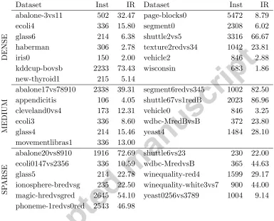
4. Experimental setup
Table 2: Description of the real-world two-class datasets used in the experimental study. This table lists the number of instances (Inst) and the IR of the dataset, measuring the degree of imbalance between the majority and minority classes.
Dataset Inst IR Dataset Inst IR
DENSE
abalone-3vs11 502 32.47 page-blocks0 5472 8.79
ecoli4 336 15.80 segment0 2308 6.02
glass6 214 6.38 shuttle2vs5 3316 66.67
haberman 306 2.78 texture2redvs34 1042 23.81
iris0 150 2.00 vehicle2 846 2.88
kddcup-bovsb 2233 73.43 wisconsin 683 1.86 new-thyroid1 215 5.14
MEDIUM
abalone17vs78910 2338 39.31 segment6redvs345 1002 82.50 appendicitis 106 4.05 shuttle67vs1redB 2023 86.96 cleveland0vs4 173 12.31 vehicle0 846 3.25 ecoli3 336 8.60 wdbc-MredBvsB 372 23.80
glass4 214 15.46 yeast4 1484 28.10
movementlibras1 336 13.00
SP
ARSE
abalone20vs8910 1916 72.69 shuttle6vs23 230 22.00 ecoli0147vs2356 336 10.59 wdbc-MredvsB 365 44.63 glass5 214 22.78 winequality-red4 1599 29.17 ionosphere-bredvsg 235 22.50 winequality-white3vs7 900 44.00 magic-hredvsgred 2645 54.10 yeast0256vs3789 1004 9.14 phoneme-1redvs0red 2543 46.98
for imbalanced classification to which EPRENNID is compared (Section 4.2), the evaluation measures (Section 4.3) and the statistical tests that we used (Section 4.4).
4.1. Datasets
We have selected 35 two-class imbalanced datasets on which all methods are executed. They were constructed by taking real-world datasets avail-able from the UCI [59] or KEEL dataset [60] repositories and consequently merging or removing classes until only two remain. This procedure is com-mon practice and has been used in other experimental studies as well (e.g. [2, 48, 52, 61]).
further divided the datasets into three subgroups, dense,mediumandsparse, which represent different degrees of difficulty to recognize minority elements. Minority instances in dense datasets are grouped closely together, while they are more spread out in sparse datasets.
Inspired by [62], we use the local neighborhood of minority elements to consider them as safe, borderline, rare or outliers. In this work, we propose an alternative definition that is more conservative than the one used in [62]. For each minority instance, we determine its five nearest neighbors in the dataset and denote it as:
• Safe: the five nearest neighbors of this instance all belong to the mi-nority class.
• Borderline: the instance has one or two majority class elements among its five nearest neighbors.
• Rare: the instance has three or four of its five nearest neighbors be-longing to the majority class.
• Outlier: all five nearest neighbors of the instance belong to the majority class.
The three groups of datasets are constructed based on the division of their minority instances among these four types.
• In a dense dataset, at least half of the minority elements are safe or
borderline.
• On the other hand, when more than half of the minority instances are
rare elements or outliers, the dataset is considered sparse.
4.2. Methods
We have chosen a number of popular, well-performing data sampling methods to compare our model with. Preprocessing methods are used in conjunction with a later classification step. Since the base classification in EPRENNID is performed by the kNN classifier, we have opted to use it for the other data sampling methods as well for a fair comparison.
Below, we provide a short descriptive overview, including specifications with regard to their parameter settings. A specific choice of parameters over the different data sources may result in better performance, but our purpose here is to analyze the general performance of the techniques without a time-consuming parameter tuning step. Their operations should provide good enough results even though the parameters are not optimized for a particular problem. For this reason, we always use the default values recommended by their developers.
• Borderline-SMOTE2 (Border2, [31]): this oversampling procedure is a modification of SMOTE. It uses minority elements located near the decision boundaries as seeds for the construction of artificial instances. Artificial minority elements are introduced on the line segment between the seed instance and a randomly selected element from among their
k nearest positive neighbors. For each seed, one synthetic element is also generated on the line segment connecting it to its nearest negative neighbor.
• SMOTE-TL (SMT-TL, [9]): a Tomek Link (TL) is defined as a pair of opposite class elements which are located more closely to each other than to any other element in the dataset. The SMOTE-TL method consists of first applying SMOTE and afterward removing all pairs of elements that form a TL.
• SMOTE-RSB∗ (SMT-RSB, [64]): similar to SMOTE-TL, this method
first applies SMOTE on the dataset and afterward removes certain instances. All original instances are automatically retained, but the synthetic elements are required to belong to the rough lower approxi-mation [65] of the minority class. If they do not satisfy this criterion, they are removed.
[66] to remove noisy negative instances. When a negative element is misclassified by 3NN, it is removed from the dataset. When a positive instance is misclassified by the 3NN rule, all of the negative instances contributing to this misclassification are removed.
• Spider2 [35]: this is a hybrid data sampling method. It has a number of options to be set, where we have chosen the best ones put forward by [35]. In a first phase, negative instances that are misclassified by 3NN are relabeled as positive. Secondly, a number of duplicates of misclassified positive elements are added to the dataset.
• SSMAImb (Section 3): we have also included our modified SSMAImb
al-gorithm described above, leaving out the PG optimization step and the ensemble classification procedure. This allows us to determine whether the added complexity of the latter two steps improves the performance of SSMAImb or whether the actual strength of our model lies in the PS
step alone.
• IPADE-ID (IPADE, [18]): this is a previously proposed method for imbalanced classification using DE, making it an interesting competitor of EPRENNID. It is an extension of the IPADE method [67] to the imbalanced domain. In both the internal workings as well as the final classification step of IPADE-ID, we are using the kNN classifier. This makes for a fair comparison with EPRENNID and the data sampling methods, as they use kNN as well.
• SMOTEBagging [45]: this bagging procedure constructs bootstrap sam-ples of the training set by applying the SMOTE oversampling method. The resampled version of the majority class is always obtained via random resampling. In sampling the minority class for a bootstrap sample, a given percentage is obtained via random resampling, while the other part is constructed by creating synthetic minority instances with SMOTE. The percentage of random resampling is varied between the different bootstrap samples. A balance between the two classes is guaranteed in each sample.
• SMOTEBoost [44]: this ensemble method uses SMOTE in each iter-ation of the AdaBoost.M2 boosting algorithm [69]. The oversampling step creates synthetic minority elements in order to better represent previously misclassified minority instances, thereby implicitly increas-ing their weights in the current interation.
• EUSBoost [48]: Similarly to SMOTEBoost, EUSBoost embeds the EUS method described above in AdaBoost.M2. In each boosting round, the undersampling step reduces the majority class to a subset.
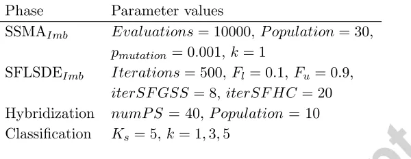
The parameter settings of EPRENNID are presented in Table 3. SSMAImb
is a modified version of SSMA and we have used the same default parameters as the latter method, as proposed in [27]. In the PG step, we use the default parameters used in [23] for SFLSDEImb. For more detail on these parameter
values, we refer to [23] and [28]. In the hybridization step, we use 40 popu-lations of 10 individuals each. The popupopu-lations are kept small on purpose, to avoid that they all converge to the same solution, which would result in a loss of diversity. In order to provide a more global picture, we have set k to 1, 3 and 5 for the kNN classifier used in the final classification step.
4.3. Evaluation measures
Table 3: Parameter settings for the EPRENNID method.
Phase Parameter values
SSMAImb Evaluations= 10000,P opulation= 30,
pmutation= 0.001, k= 1
SFLSDEImb Iterations= 500, Fl = 0.1,Fu = 0.9,
iterSF GSS= 8, iterSF HC = 20
Hybridization numP S = 40,P opulation = 10 Classification Ks= 5, k= 1,3,5
4.4. Statistical analysis
In order to test for significance in the observed differences in the exper-imental results, we apply non-parametric statistical tests, as recommended in [70, 71]. We use the Friedman test [72] to verify whether any significant differences in performance are present among a group of methods. When the p-value of this test is lower than a specified significance level α, the null hypothesis of equivalent performance is rejected and we conclude that significant differences exist among the methods.
To determine where these significant differences occur, we apply the Ne-menyi post hoc test. In this test, the performance of two classifiers is signifi-cantly different only if their average ranks differ by a certain critical distance. The critical distance depends on the number of algorithms, the number of datasets and the critical value for a significance level provided by a Studen-tized range statistic. The result of the Nemenyi post hoc test is plotted with an average ranks diagram. The ranks are depicted on the axis, so that the best algorithms are at the right side of the diagram. A line with the length of the critical distance is drawn between those algorithms that do not differ significantly (in performance) for a significance level of α = 0.05. More in-formation about these tests and other statistical procedures can be found at http://sci2s.ugr.es/sicidm/.
5. Experimental results
results. We divide the further discussion of these results into two main parts. Section 5.3 compares EPRENNID with data sampling models, while Section 5.4 presents a comparison with ensemble-based models. Due to the extent of our experimental analysis, we are unable to list all results here. The complete results are reported on the associated web page http: //www.cwi.ugent.be/sarah.php.
5.1. A note on reduction
Before discussing the classification performance of our proposal in detail, we briefly note that the average reduction of the prototype sets in the ensem-ble in EPRENNID is 0.6413 (dense), 0.8123 (medium), 0.8904 (sparse) and 0.7733 (all). The global reduction after the SSMAImb step however is only
0.3820 (dense), 0.6108 (medium), 0.7393 (sparse) and 0.5662 (all). The global reduction is computed by taking the union of the prototype sets and compar-ing it to the full traincompar-ing set. Since we guarantee a level of diversity between the sets in the ensemble, the global reduction is noticeably lower than the average reduction. Since reduction is not the most relevant measure for our method, we do not further compare these values with those obtained by the data sampling methods and instead focus on the classification performance.
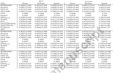
5.2. Overview of results
In Table 4, we present a compact overview of the classification results of all included methods, using both the AUC and g mean as evaluation measures. As noted above, we consider three different values for k in the classification step of EPRENNID. The data sampling methods are combined with 1NN, 3NN and 5NN. The ensemble methods are only evaluated for
k = 1, as motivated in Section 5.4. We list the average values for each dataset group, combined with the average standard deviation over 10 runs where applicable. The reader can refer back to this table throughout our discussion in the remainder of the paper. The full results can be consulted at http://www.cwi.ugent.be/sarah.php.
5.3. Comparison with data sampling models
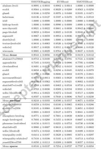
Table 4: Overview of all classification results
AUC g mean
1NN Dense Medium Sparse Dense Medium Sparse EPRENNID 0.9626±0.003 0.9514±0.004 0.9020±0.011 0.9289±0.006 0.8651±0.017 0.7372±0.018 Border2 0.9291±0.004 0.8135±0.018 0.6926±0.053 0.9294±0.004 0.8130±0.019 0.693±0.056 SMT-TL 0.9313±0.005 0.8575±0.019 0.7763±0.029 0.9311±0.005 0.8574±0.020 0.776±0.030 SMT-RSB 0.9267±0.004 0.8154±0.026 0.7084±0.043 0.9269±0.004 0.8160±0.029 0.708±0.045 NCR 0.9263 0.8358 0.7400 0.9228 0.8067 0.747 Spider2 0.9181 0.8027 0.7110 0.9137 0.6425 0.568 SSMAImb 0.9326±0.005 0.8722±0.017 0.7873±0.034 0.9318±0.005 0.8712±0.018 0.782±0.035
IPADE 0.9190±0.009 0.8795±0.022 0.8111±0.026 0.9168±0.010 0.8687±0.032 0.783±0.044 EUS 0.9276±0.007 0.8737±0.014 0.7836±0.028 0.9272±0.008 0.8734±0.015 0.785±0.030 SMOTEBagging 0.9544±0.006 0.9210±0.010 0.8516±0.014 0.9285±0.007 0.8536±0.013 0.717±0.016 SMOTEBoost 0.9419±0.014 0.8671±0.036 0.7797±0.036 0.8441±0.061 0.3677±0.148 0.262±0.096 EUSBoost 0.9329±0.015 0.8580±0.056 0.7254±0.073 0.8828±0.050 0.6250±0.227 0.349±0.174 3NN
EPRENNID 0.9637±0.002 0.9522±0.006 0.8845±0.013 0.9217±0.004 0.8752±0.014 0.7412±0.028 Border2 0.9367±0.010 0.8372±0.049 0.7257±0.069 0.9368±0.011 0.8378±0.052 0.7257±0.073 SMT-TL 0.9399±0.007 0.8844±0.029 0.8161±0.037 0.9397±0.008 0.8843±0.030 0.8166±0.040 SMT-RSB 0.9409±0.009 0.8661±0.031 0.7431±0.049 0.9406±0.009 0.8663±0.032 0.7435±0.052 NCR 0.9393 0.8847 0.7825 0.9152 0.7628 0.5531 Spider2 0.9487 0.8624 0.7484 0.9182 0.7844 0.6111 SSMAImb 0.9417±0.011 0.8985±0.034 0.8150±0.044 0.9350±0.012 0.8885±0.035 0.7972±0.048
IPADE 0.8575±0.035 0.7876±0.058 0.7447±0.052 0.4011±0.225 0.5416±0.210 0.4436±0.205 EUS 0.9378±0.013 0.8967±0.028 0.7961±0.044 0.9374±0.014 0.8967±0.030 0.7959±0.047 5NN
EPRENNID 0.9601±0.002 0.9457±0.006 0.8763±0.012 0.9137±0.006 0.8651±0.019 0.6921±0.038 Border2 0.9396±0.014 0.8553±0.052 0.7488±0.071 0.9397±0.014 0.8553±0.055 0.7488±0.075 SMT-TL 0.9443±0.010 0.9019±0.019 0.8302±0.039 0.9439±0.011 0.9015±0.020 0.8298±0.042 SMT-RSB 0.9429±0.012 0.8816±0.033 0.7584±0.058 0.9430±0.013 0.8821±0.035 0.7589±0.062 NCR 0.9479 0.8998 0.7982 0.9048 0.6954 0.4496 Spider2 0.9466 0.8851 0.7662 0.9189 0.7847 0.6267 SSMAImb 0.9414±0.017 0.8915±0.042 0.7967±0.057 0.9331±0.018 0.8767±0.047 0.7776±0.062
IPADE 0.8760±0.032 0.8153±0.048 0.7582±0.046 0.4746±0.220 0.6184±0.164 0.5153±0.176 EUS 0.9387±0.017 0.9001±0.033 0.7868±0.051 0.9378±0.018 0.8999±0.035 0.7873±0.056
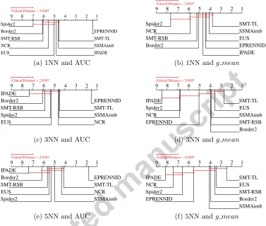
the best-performing method is printed in bold. In order not to clutter this discussion, we do not list the complete results of the g meanmeasure nor for 3NN and 5NN. The results of the statistical analyses relevant to this section can be found in Figure 2, plotting the average ranks diagrams. We note that we have taken the entire group of 35 datasets to perform the statistical anal-ysis, rather than doing this group-wise, as the sizes of the groups are rather small. We discuss the results of the two evaluation measures, AUC and
g mean, separately in Sections 5.3.1 and 5.3.2 respectively. In Section 5.3.3, we compare EPRENNID to the data sampling methods in terms of their runtime.
5.3.1. Analysis of the AUC results
9 8 7 6 5 4 3 2 1
EPRENNID SMT-TL SSMAimb IPADE EUS
NCR SMT-RSB Border2 Spider2
Critical Distance = 2.0307
(a) 1NN and AUC
9 8 7 6 5 4 3 2 1
SMT-TL SSMAimb EUS EPRENNID IPADE Border2
SMT-RSB NCR Spider2
Critical Distance = 2.0307
(b) 1NN andg mean
9 8 7 6 5 4 3 2 1
EPRENNID SMT-TL SSMAimb NCR EUS
Spider2 SMT-RSB Border2 IPADE
Critical Distance = 2.0307
(c) 3NN and AUC
9 8 7 6 5 4 3 2 1
SMT-TL EUS SSMAimb SMT-RSB Border2 EPRENNID
NCR Spider2 IPADE
Critical Distance = 2.0307
(d) 3NN andg mean
9 8 7 6 5 4 3 2 1
EPRENNID SMT-TL NCR SSMAimb Spider2
EUS SMT-RSB Border2 IPADE
Critical Distance = 2.0307
(e) 5NN and AUC
9 8 7 6 5 4 3 2 1
SMT-TL EUS SMT-RSB Border2 SSMAimb EPRENNID
Spider2 NCR IPADE
Critical Distance = 2.0307
[image:28.612.126.503.138.458.2](f) 5NN andg mean
Figure 2: Average ranks diagrams for AUC andg meanusing 1NN, 3NN and 5NN
classi-fiers. Better algorithms are located on the right side of the plot (rank closer to 1). Those
that differ by less than the critical distance computed for a p-value=0.05 are linked by a
red line.
EPRENNID still comes out on top.
does decrease with the difficulty of the dataset, this decrease is less prominent than for other methods. For instance, while EPRENNID only loses 0.0606, its closest competitors IPADE-ID and EUS face a decrease in AUC of about 0.1079 and 0.1440. Although their dataset-wise results are not printed here, similar conclusions can be drawn for 3NN and 5NN. This observation shows the good performance of EPRENNID for all types of class imbalance.
We note that our new PS method SSMAImb also performs tolerably well,
most prominently so for 1NN. For this classifier, it yields better results than all included data sampling methods, putting it at the same level as IPADE-ID. It is interesting to observe that SSMAImb, a true undersampling method
removing both positive and negative elements, is able to outperform un-dersampling (NCR, EUS), oversampling (Borderline-SMOTE2) and hybrid (SMOTE-TL, SMOTE-RSB, Spider2) data sampling methods. This con-stitutes clear evidence that the complete protection of the minority class, incorporated by all these methods, is not necessarily justified. Allowing the removal of minority elements, which can also be noisy or redundant, pro-vides us with an added flexibility, which makes it possible to handling class imbalance more appropriately. For higher values of k, SSMAImb remains
steadily at the top and, apart from by EPRENNID, is only improved by NCR and SMOTE-TL for 5NN. We conclude that we have proposed a strong PS method able to handle class imbalance, but it can nevertheless be further im-proved by hybridizing it with PG and including the ensemble classification. From Figure 2, we observe that, for all classifiers, our method has the best rank with respect to the AUC values. Comparing EPRENNID to the others with the Nemenyi post hoc test, we conclude that it yields significantly better results than all other methods under consideration, since none of the others is located within the critical distance of our proposal. This statement holds for all three classifiers and confirms the clear dominance of our new method over the state-of-the-art in data sampling.
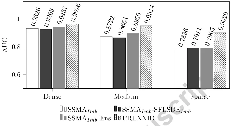
Finally, in Figure 3, we visually compare the full EPRENNID model to three partially constructed ones, in order to determine whether the added complexity of the full model increases its performance. The figure is based on the performance of 1NN evaluated by the AUC. We already observed that solely applying SSMAImb, generating a single prototype set, yields good
classification results, although they are improved upon by EPRENNID. Fur-thermore, optimizing this single subset by SFLSDEImb does not on its own
increase the performance, as presented by SSMAImb-SFLSDEImb in the
Dense Medium Sparse 0.6
0.8 1
0.9326
0.8722
0.7836 0.9269
0.8654
0.7911 0.9437
0.8950
0.7905
0.9626 0.9514
0.9020
A
UC
SSMAImb SSMAImb-SFLSDEImb
[image:30.612.111.499.126.337.2]SSMAImb-Ens PRENNID
Figure 3: Comparison of EPRENNID with partially constructed models. In SSMAImb,
only the PS step is performed. SSMAImb+SFLSDEImbis the same as EPRENNID, apart
from the important fact that only one prototype set is constructed. This comparison was done for 1NN, of which the performance was evaluated by the AUC.
to be due to the overfitting problem to which PG methods are prone [20]. We also consider the extension of SSMAImb with the ensemble approach in
EPRENNID, without optimizing the prototype sets by SFLSDEImb. This
setting is represented by SSMAImb-Ens. Although giving an improvement
over SSMAImb, it is itself clearly improved upon by introducing the
opti-mization step by PG. The optiopti-mization of multiple diverse prototype sets and their aggregation into a classification ensemble is shown to be truly worth the effort.
5.3.2. Analysis of the g mean results
With respect to the evaluation byg mean, the results are less favorable for EPRENNID, as shown in Table 4. For 1NN, we observe that EPRENNID still outperforms several state-of-the-art data sampling methods, but it is itself outperformed by the IPADE-ID method for medium and sparse datasets. The undersampling method EUS combined with 1NN yields better average results than EPRENNID as well. Our PS method SSMAImb still exhibits
In combination with 3NN, we observe that the hybrid data sampling methods SMOTE-TL and SMOTE-RSB∗ perform better than before,
plac-ing them at the same level as EPRENNID, IPADE-ID, SSMAImb and EUS.
For 5NN, the hybrid data sampling methods, especially SMOTE-TL, domi-nate. EPRENNID yields decent results, although its overall average result for
g mean is lower than that of SSMAImb. Considering this phenomenon more
closely, we observed that this is due to a decrease in performance of EPREN-NID on sparse datasets, for which its average g mean value is considerably lower than that of SSMAImb, as can be seen in Table 4. In a sparse dataset,
the minority class is severely spread out over the feature space, making it more difficult forkNN to classify them correctly, especially for higher values of k. By using the ensemble approach in EPRENNID, misclassifications can build up, resulting in a decrease in performance. We conclude that in such a setting, where higher values of k are used to classify a sparse dataset with the kNN rule, it might be more appropriate to stick to the preprocessing method SSMAImb.
In the statistical analysis of theg meanvalues (Figure 2), SMOTE-TL is assigned the best rank for all values ofk. For 1NN, 3NN and 5NN, SMOTE-TL is shown to significantly outperform NCR and Spider2. For 3NN and 5NN, it also performs significantly better than IPADE and EPRENNID. As noted above, upon closer examination it is revealed that the poor average result of EPRENNID in this case is due to an inferior performance on the sparse datasets.
Nevertheless, by taking the results of both evaluation measures into ac-count, we can conclude that our new proposal of a hybrid model, integrating PS and PG in its preprocessing step and using a weighted voting procedure in its classification, is competitive with the state-of-the-art data sampling methods as well as IPADE-ID.
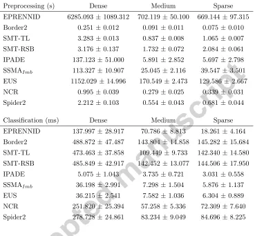
5.3.3. Runtime analysis
Table 6: Runtime results for the data sampling methods using the 1NN as classifier.
Preprocessing (s) Dense Medium Sparse
EPRENNID 6285.093±1089.312 702.119±50.100 669.144±97.315
Border2 0.251±0.012 0.091±0.011 0.075±0.010
SMT-TL 3.283±0.013 0.837±0.008 1.065±0.007
SMT-RSB 3.176±0.137 1.732±0.072 2.084±0.061
IPADE 137.123±51.000 5.891±2.852 5.697±2.798
SSMAImb 113.327±10.907 25.045±2.116 39.547±3.501
EUS 1152.029 ±14.996 170.549±2.473 129.586±2.667
NCR 0.995±0.039 0.279±0.025 0.339±0.031
Spider2 2.212±0.103 0.554±0.043 0.681±0.044
Classification (ms) Dense Medium Sparse
EPRENNID 137.997±28.917 70.786±8.813 18.261±4.164
Border2 488.872±47.487 143.804±14.858 145.282±15.684
SMT-TL 473.463±37.858 109.449±9.733 142.340±14.580
SMT-RSB 485.849±42.917 142.452±13.077 144.506±17.950
IPADE 5.075±1.043 3.735±0.721 3.031±0.558
SSMAImb 36.198±2.991 7.298±1.504 5.876±1.137
EUS 36.215±2.541 7.582±1.036 6.304±0.889
NCR 251.820±25.394 57.258±5.336 72.309±7.640
Spider2 278.728±24.861 83.234±9.049 84.696±8.225
4 3 2 1
EPRENNID SMOTEBagging
SMOTEBoost EUSBoost
Critical Distance = 0.79281
(a) AUC
4 3 2 1
EPRENNID SMOTEBagging
EUSBoost SMOTEBoost
Critical Distance = 0.79281
[image:33.612.114.514.134.234.2](b)g mean
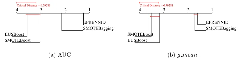
Figure 4: Average ranks diagrams for AUC and g meanusing the 1NN classifier for the
ensemble-based models. Better algorithms are located on the right side of the plot (rank
closer to 1). Those that differ by less than the critical distance computed for ap-value=0.05
are linked by a red line.
terms of classification performance. Nevertheless, if the required runtime of EPRENNID cannot be afforded by the user, he can resort to our SSMAImb
method instead, which has a good classification performance (Table 4) and a reasonable runtime. In Section 5.4, we compare the runtime of EPRENNID to other ensemble methods, which makes for a fairer comparison.
5.4. Comparison with ensemble-based models
In this section, we compare EPRENNID to other ensemble-based models for imbalanced classification described in Section 4.2. We note that to estab-lish a fair comparison between the different ensemble methods, we use the 1NN technique as base classifier in all cases. All ensembles use the same num-ber of classifiers internally, set to the same value as the numnum-ber of prototype sets used by EPRENNID.
Table 7 collects the results on all datasets, evaluating the classification performance of the 1NN classifier in terms of the AUC measure. As we saw in the comparison of EPRENNID with data sampling methods, our proposal dominates the other methods for all datasets groups. Its dominance becomes more apparent for increasing difficulty of the dataset, going from the dense, to the medium, to the sparse group. Figure 4 depicts the statistical evaluation by means of average ranks diagrams. It shows that EPRENNID significantly outperforms SMOTEBagging, SMOTEBoost and EUSBoost with respect to the AUC obtained over all datasets. Considering the evaluation by g mean
Table 7: AUC results for the ensemble-based models using 1NN as base classifier, with standard deviations over 10 runs
Table 8: Runtime results for the ensemble-based methods.
Building (s) Dense Medium Sparse
EPRENNID 6285.093 ±1089.312 702.119±50.100 669.144±97.315
SMOTEBagging 2687.683±438.284 1258.393 ±86.260 1619.857±111.510
SMOTEBoost 6895.590 ±1112.069 2850.102±252.999 3871.108±386.373
EUSBoost 5901.096±418.371 1053.477±143.183 1158.963 ±58.233
Classification (ms) Dense Medium Sparse
EPRENNID 137.997±28.917 70.786±8.813 18.261±4.164
SMOTEBagging 25.924±6.102 28.398±5.536 25.089±4.736
SMOTEBoost 50.297±10.121 50.409±8.781 44.000±8.653
EUSBoost 7.392±0.990 2.968±0.746 1.798±0.224
We also comment on the computational complexity of EPRENNID com-pared to the other ensembles. In order to do so, Table 8 presents the average group-wise runtime required by each method, differentiating between build-ing and classification times. The buildbuild-ing time refers to the necessary time to create the ensemble, while the classification time involves the average time spent to label a test instance. The former is given in seconds, the latter in milliseconds. We observe that both are comparable between the four mod-els. The classification time of EPRENNID is slightly higher than that of the other models, which is due to the target-specific weight construction for the prototype sets in the ensemble. This component is not present in the other ensemble-based methods. Nevertheless, taking the prediction results into ac-count, EPRENNID may be preferred over the other three models, especially for imbalanced datasets with higher difficulty. Indeed, we observe that for the medium and sparse groups, the average building time of EPRENNID is the lowest among the four models and its classification performance is highly superior as well, as indicated in Table 4 and Figure 4.
6. Conclusion and future work
completely protect the minority class, the proposed model can reduce both majority and minority class examples, when necessary.
In our experiments, we were able to show that our new PS method out-performs several popular data sampling methods used in imbalanced clas-sification. This shows that strenuously protecting minority elements is not necessarily the best option and including more flexible heuristics can prove to be more useful in dealing with class imbalance.
Secondly, we proposed to select not one, but a diverse set of well-performing prototype sets generated by the PS method. These sets were further opti-mized by a differential evolution scheme. As a final step, we set up an ensemble with the optimized prototype sets. The implemented voting strat-egy allows to assign prototype sets performing well in the neighborhood of a target instance a larger weight in its classification.
Our model does not aim to perform a significant data reduction of the dataset, but to increase the overall performance. Our experiments showed that it significantly outperforms state-of-the-art data sampling methods and ensemble-based methods, as well as a previous proposal using differential evolution in imbalanced classification, for the AUC measure. However, for the g mean measure, it provides a similar performance in comparison to state-of-the-art models. In terms of computational cost, it is fairly similar to other ensemble-based methods.
As future work, we consider to study how an artificial injection of noisy examples may affect the behavior of our proposal. Moreover, we also in-tend to exin-tend the presented approach to use other classifiers, like decision trees and support vector machines. This will require the development of cus-tom prototype reduction methods for these classifiers in the class imbalance domain.
Acknowledgments
[1] Y. Lee, P. Hu, T. Cheng, T. Huang, W. Chuang, A preclustering-based ensemble learning technique for acute appendicitis diagnoses, Artificial intelligence in medicine 58 (2) (2013) 115–124.
[2] H. Yu, J. Ni, J. Zhao, ACOSampling: An ant colony optimization-based undersampling method for classifying imbalanced dna microarray data, Neurocomputing 101 (2013) 309–318.
[3] C. Seiffert, T. Khoshgoftaar, J. Van Hulse, A. Folleco, An empirical study of the classification performance of learners on imbalanced and noisy software quality data, Information Sciences 259 (2014) 571–595. [4] E. Alpaydin, Introduction to Machine Learning, 2nd Edition, MIT Press,
Cambridge, MA, 2010.
[5] N. Japkowicz, The class imbalance problem: Significance and strate-gies, in: Proceedings of the 2000 International Conference on Artificial Intelligence, Vol. 1, 2000, pp. 111–117.
[6] H. He, E. Garcia, Learning from imbalanced data, IEEE Transactions on Knowledge and Data Engineering 21 (9) (2009) 1263–1284.
[7] V. L´opez, A. Fern´andez, S. Garc´ıa, V. Palade, F. Herrera, An insight into classification with imbalanced data: Empirical results and current trends on using data intrinsic characteristics, Information Sciences 250 (2013) 113–141.
[8] M. Lin, K. Tang, X. Yao, Dynamic sampling approach to training neural networks for multiclass imbalance classification, IEEE Transactions on Neural Networks and Learning Systems 24 (4) (2013) 647–660.
[9] G. Batista, R. Prati, M. Monard, A study of the behavior of several methods for balancing machine learning training data, SIGKDD Explo-rations 6 (1) (2004) 20–29.
[10] N. Chawla, K. Bowyer, L. Hall, W. Kegelmeyer, SMOTE: Synthetic minority over-sampling technique, Journal of Artificial Intelligence Re-search 16 (2002) 321–357.
[12] D. Hand, V. Vinciotti, Choosing k for two-class nearest neighbour classi-fiers with unbalanced classes, Pattern Recognition Letters 24 (9) (2003) 1555–1562.
[13] D. R. Wilson, T. R. Martinez, Reduction techniques for instance-based learning algorithms, Machine Learning 38 (3) (2000) 257–286.
[14] I. Kononenko, M. Kukar, Machine Learning and Data Mining: Introduc-tion to Principles and Algorithms, Horwood Publishing Limited, 2007. [15] I. Triguero, D. Peralta, J. Bacardit, S. Garc´ıa, F. Herrera, MRPR: A
mapreduce solution for prototype reduction in big data classification, Neurocomputing 150, Part A (0) (2015) 331 – 345. doi:10.1016/j. neucom.2014.04.078.
[16] S. Garc´ıa, F. Herrera, Evolutionary undersampling for classification with imbalanced datasets: Proposals and taxonomy, Evolutionary Computa-tion 17 (3) (2009) 275–306.
[17] A. de Haro-Garcia, N. Garcia-Pedrajas, A scalable method for instance selection for class-imbalance datasets, in: Proceedings of the 11th In-ternational Conference on Intelligent Systems Design and Applications (ISDA’11), 2011, pp. 1383–1390.
[18] V. L´opez, I. Triguero, C. Carmona, S. Garc´ıa, F. Herrera, Addressing imbalanced classification with instance generation techniques: IPADE-ID, Neurocomputing 126 (2014) 15–28.
[19] S. Garc´ıa, J. Derrac, J. Cano, F. Herrera, Prototype selection for nearest neighbor classification: Taxonomy and empirical study, IEEE Transac-tions on Pattern Analysis and Machine Intelligence 34 (3) (2012) 417– 435.
[20] I. Triguero, J. Derrac, S. Garcia, F. Herrera, A taxonomy and experi-mental study on prototype generation for nearest neighbor classification, IEEE Transactions on Systems, Man, and Cybernetics, Part C: Appli-cations and Reviews 42 (1) (2012) 86–100.
[22] S. Das, P. Suganthan, Differential evolution: A survey of the state-of-the-art, IEEE Transactions on Evolutionary Computation 15 (1) (2011) 4–31.
[23] I. Triguero, S. Garc´ıa, F. Herrera, Differential evolution for optimizing the positioning of prototypes in nearest neighbor classification, Pattern Recognition 44 (4) (2011) 901–916.
[24] T. Cover, P. Hart, Nearest neighbor pattern classification, Information Theory, IEEE Transactions on 13 (1) (1967) 21–27.
[25] J. F. Dez-Pastor, J. J. Rodrguez, C. Garca-Osorio, L. I. Kuncheva, Random balance: Ensembles of variable priors classifiers for imbal-anced data, Knowledge-Based Systems 85 (2015) 96 – 111. doi:http: //dx.doi.org/10.1016/j.knosys.2015.04.022.
[26] D. Aha, Editorial, in: Lazy Learning, Springer, 1997, pp. 7–10.
[27] S. Garc´ıa, J. Cano, F. Herrera, A memetic algorithm for evolutionary prototype selection: A scaling up approach, Pattern Recognition 41 (8) (2008) 2693–2709.
[28] F. Neri, V. Tirronen, Scale factor local search in differential evolution, Memetic Computing 1 (2) (2009) 153–171.
[29] R. Storn, K. Price, Differential evolution–a simple and efficient heuristic for global optimization over continuous spaces, Journal of global opti-mization 11 (4) (1997) 341–359.
[30] J. Laurikkala, Improving identification of difficult small classes by bal-ancing class distribution, in: 8th Conference on AI in Medicine in Eu-rope, Vol. 2001 of Lecture Notes on Computer Science, Springer Berlin / Heidelberg, 2001, pp. 63–66.
[32] S. Barua, M. Islam, X. Yao, K. Murase, et al., MWMOTE–majority weighted minority oversampling technique for imbalanced data set learn-ing, IEEE Transactions on Knowledge and Data Engineering 26 (2) (2014) 405–425.
[33] C. Bunkhumpornpat, K. Sinapiromsaran, C. Lursinsap, Safe-level-SMOTE: Safe-level-synthetic minority over-sampling technique for han-dling the class imbalanced problem, in: Pacific-Asia Conference on Knowledge Discovery and Data Mining, Vol. 5476 of Lecture Notes on Computer Science, Springer-Verlag, 2009, pp. 475–482.
[34] J. Stefanowski, S. Wilk, Selective pre-processing of imbalanced data for improving classification performance, in: 10th International Conference in Data Warehousing and Knowledge Discovery, Vol. 5182 of Lecture Notes on Computer Science, Springer, 2008, pp. 283–292.
[35] K. Napierala, J. Stefanowski, S. Wilk, Learning from imbalanced data in presence of noisy and borderline examples, in: 7th International Con-ference on Rough Sets and Current Trends in Computing, 2010, pp. 158–167.
[36] K. Veropoulos, C. Campbell, N. Cristianini, Controlling the sensitivity of support vector machines, in: Proceedings of the international joint conference on artificial intelligence, 1999, pp. 55–60.
[37] S. Datta, S. Das, Near-bayesian support vector machines for imbalanced data classification with equal or unequal misclassification costs, Neu-ral Networks 70 (2015) 39 – 52. doi:http://dx.doi.org/10.1016/j. neunet.2015.06.005.
[38] C. Castro, A. Braga, Novel cost-sensitive approach to improve the mul-tilayer perceptron performance on imbalanced data, IEEE Transactions on Neural Networks and Learning Systems 24 (6) (2013) 888–899. [39] B. Krawczyk, M. Galar, ukasz Jele, F. Herrera, Evolutionary
under-sampling boosting for imbalanced classification of breast cancer ma-lignancy, Applied Soft Computing 38 (2016) 714 – 726. doi:http: //dx.doi.org/10.1016/j.asoc.2015.08.060.