Classification of large acoustic datasets using machine learning and crowdsourcing : application to whale calls

Classification of large acoustic datasets using machine

learning and crowdsourcing: Application to whale calls

Lior Shamira)and Carol Yerby

Lawrence Technological University, 21000 Ten Mile Road, Southfield, Michigan 48075

Robert Simpson

University of Oxford, Denys Wilkinson Building, Keble Road, Oxford, OX1 3RH, United Kingdom

Alexander M. von Benda-Beckmann

The Netherlands Organization for Applied Scientific Research, P.O. Box 96864, The Hague, Zuid Holland, 2509 JG, The Netherlands

Peter Tyack, Filipa Samarra, and Patrick Miller

University of St. Andrews, St. Andrews, Fife, KY16 9ST, Scotland, United Kingdom

John Wallin

Middle Tennessee State University, 1301 East Main Street, Murfreesboro, Tennessee 37130

(Received 7 April 2013; revised 12 November 2013; accepted 17 December 2013)

Vocal communication is a primary communication method of killer and pilot whales, and is used for transmitting a broad range of messages and information for short and long distance. The large variation in call types of these species makes it challenging to categorize them. In this study, sounds recorded by audio sensors carried by ten killer whales and eight pilot whales close to the coasts of Norway, Iceland, and the Bahamas were analyzed using computer methods and citizen scientists as part of the Whale FM project. Results show that the computer analysis automatically separated the killer whales into Icelandic and Norwegian whales, and the pilot whales were separated into Norwegian long-finned and Bahamas short-finned pilot whales, showing that at least some whales from these two locations have different acoustic repertoires that can be sensed by the computer analysis. The citizen science analysis was also able to separate the whales to locations by their sounds, but the separation was somewhat less accurate compared to the computer method.

VC _{2014 Acoustical Society of America. [http://dx.doi.org/10.1121/1.4861348]}

PACS number(s): 43.80.Ka, 43.80.Lb [JJF] Pages: 953–962

I. INTRODUCTION

Whales and dolphins produce a series of whistles, clicks, and other sounds to survey their surroundings, hunt for food, and communicate with each other (Schevill and Watkins 1966; Ford, 1989). Killer whales (Orcinus orca) and pilot whales (Globicephala spp.) are species of dolphins. Killer whales, which are the largest dolphin species, have been studied in more detail than pilot whales (Ottensmeyer and Whitehead, 2003), and some populations have been con-tinually studied for over three decades (Ford et al., 2000). Animals within socially stable family units known as “pods” share a unique repertoire (also known as dialect) of stereo-typed calls, which are comprised of a complex pattern of pulsed and tonal elements that may be inherited genetically, culturally, or learned from members of the group (Miller and Bain, 2000). Pods that share any parts of their repertoire are grouped into acoustic clans (Yurket al., 2002;Milleret al., 2004), and calls of killer whales have been collected and categorized for understanding the function or usage patterns of the calls. It is believed that pilot whales live in matrilineal groups or pods similar to killer whales where offspring stay

with their mother, but less is known about whether pilot whale call structure may follow matrilineal bonds (Sayigh

et al., 2012).

Studies have supported the hypothesis that pod-specific calling behavior in killer whales is due to the differences between matrilineal units that accumulate over time (Ford, 1991;Miller and Bain, 2000). It has also been observed that communities may share whistle types. Studies reported that pods of killer whales that have different call repertoires may use the same set of stereotyped whistles (Rieschet al., 2006). This communication might provide a way for the whales to recognize each other on a community-level that facilitates association and affiliation of different clan members, which otherwise use distinct calls.Rieschet al.(2006)suggest that vocal learning occurs between groups and plays an important role in the spread of whistle types.

For both killer and pilot whales, the complex sounds they produce can be labeled as “calls” and the tonal sounds as “whistles” (Samarraet al., 2010;Sayighet al., 2012). The whistles appear to play an important role in the whales’ underwater acoustic communication when socializing, and the calls have been recognized as a form of long-range com-munication (Thomsenet al., 2002;Miller, 2006). The click-ing sounds have been found to be used for echolocation (Barrett-Lennard et al., 1996), which allows the whale to navigate its underwater surroundings and search for prey.

a)_{Author to whom correspondence should be addressed. Electronic mail:}

Researchers are not the only ones interested in understand-ing whale communication. It has been determined that harbor seals in the northeastern Pacific Ocean can distinguish between the vocalization of local fish-eating killer whales and the tran-sient mammal-eating killer whales. Clearly, the ability of a prey species to identify certain elements in the communication of its predator can be vital for survival. While many studies have focused on detailed analyses of vocalizations within a population of killer or pilot whales (Ottensmeyer and Whitehead, 2003; Ford et al., 2000), fewer have sought to resolve the extent to which closely related species or subpopu-lations of a single species might vary in their sound production behavior. Distinguishing between species and populations within species is important for use of acoustic data in survey methodologies (Oswaldet al., 2003).

Classification of killer whale and pilot whale calls is usu-ally performed by a small group of experts who inspect the sound recordings. However, devices such as hydrophones deployed from ships, attached to buoys, or mounted on the seafloor (Glotin et al., 2008; van Parijs et al., 2009; von Benda-Beckmann et al., 2010), or digital acoustic recording tags (DTAGs) placed on marine mammals (Johnson and Tyack, 2003;Tyacket al., 2006) are used to acquire increas-ingly large datasets of whale sound samples. The increasing size of acoustic databases makes the process of expert-based auditing increasingly time consuming and requires new analy-sis approaches that are capable of dealing with such large databases. Different approaches for analyzing large datasets are being developed. For instance, methods for processing these large datasets include supervised machine learning such as neural networks (Deeckeet al., 1999), but the high dimen-sionality makes accurate analysis of sound data challenging (Tzanetakis and Cook, 2002). Recently, a citizen science pro-ject, Whale FM, has constructed a large database of killer whale and pilot whale calls with the aim of testing the possi-bility of using crowdsourcing to process large acoustic data-sets. Citizen science can be defined as scientific research done with the participation of non-professional scientists, in most cases voluntarily, performing tasks that do not require formal training or experience in science. These tasks can include the collection of data, basic analysis of scientific data, develop-ment and operation of basic scientific equipdevelop-ment, placedevelop-ment of sensors and other scientific equipment in rarely visited locations, and more. The non-scientist participants of these projects are referred to as “citizen scientists.”

The purpose of Whale FM is to demonstrate how both citizen science analysis and machine learning can be used to analyze and categorize a large dataset of calls of killer and pilot whales. We test whether these methods can be used to analyze large call repositories and identify differences between and within species based on the variation in geo-graphical locations of the whales.

II. MATERIALS AND METHODS A. Whale FM

Whale FM is a citizen science project from Zooniverse and Scientific American. Built originally for Galaxy Zoo 2, the Zooniverse software and its successive versions have

now been used by more than 20 different projects across a range of research disciplines. The Zooniverse toolset is designed primarily as a way of serving a large collection of “assets” (audio/visual spectrograms, in the case of Whale FM) to a user interface, and collecting back user-generated interactions with these assets.

Galaxy Zoo (Lintott et al., 2008; Lintott et al., 2011) and the larger suite of Zooniverse projects have successfully built a large community of volunteers eager to participate in scientific activities. Over 800 000 registered volunteers have contributed to Zooniverse projects at the time of writing.

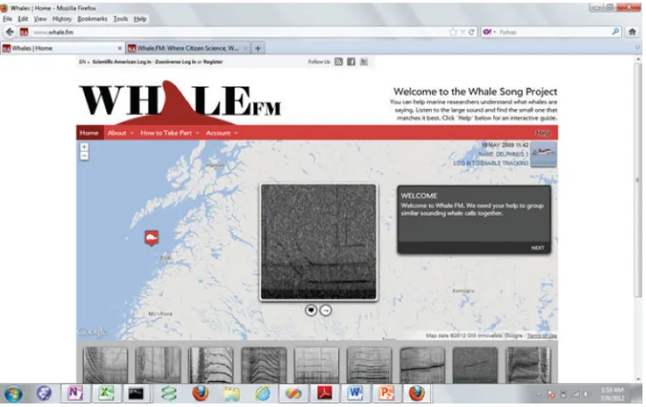
Upon viewing the Whale FM web site, volunteers see a large spectrogram and a series of smaller thumbnail grams beneath it. The citizen scientist clicks on the spectro-gram to listen to its corresponding sound. It also shows where the whale sound was recorded on a map. The citizen scientist then compares the sound with the series of 36 whale calls beneath to find a matching call. The series of 36 calls from which the volunteer chooses are selected randomly, but the selection is limited to calls of the same species and excludes calls that are clearly different from the target call as deter-mined by the length of the call and its base frequency. If a matched call is declared, it is saved in the project’s database. Calls can also be manually removed from the list (to enable easier filtering by the volunteers) and these “anti-matches” are also recorded. Anti-matches annotated by a certain citizen sci-entist will not remove the same calls from the list of calls given to another citizen scientist. Figure 1 shows the user interface used by the citizen scientists when they compare a certain main whale call to a set of matching calls.

This method can be used to analyze a large set of audio files far faster than any single researcher or group of researchers. The approach is limited by the ability of untrained volunteers to accurately recognize the whale calls. However, the Zooniverse projects have shown that enlisting these citizen scientists via the Internet is a powerful way to analyze large amounts of data. Enlisting citizen scientists enables researchers to extend human classification to com-plex data, having each sample examined by a large number of independent classifiers. Tapping into the “wisdom of the crowd” effect, researchers can rely on the consensus of a group of non-experts, which is often more accurate than the testimony of a single expert. Much success has been had with other Zooniverse projects in this regard, notably Galaxy Zoo (Lintott et al., 2008), Planet Hunters (Fischer et al., 2011), and the Milky Way Project (Simpsonet al., 2012). In all cases, the classifications of a large number of volunteers have led to the creation of data catalogs superior to those created by their expert predecessors.

B. Data

The audio samples were collected using several record-ing devices. Hydrophone arrays were towed by ships, and other hydrophone systems were deployed from buoys or overboard from stationary vessels and towed by moving ves-sels near Iceland and Norway (Milleret al., 2004; Nousek

meters away from the subjects. Several different arrays were used. A 16-element array recorded to a Pioneer (Kawasaki, Kanagawa, Japan) D-9601 (frequency response 0.020–44 kHz, 60.5 dB) and resampled to 96 kHz with an Edirol (Hamamatsu, Japan) FA-101 soundcard (frequency response 0.02–40 kHz, þ0/2 dB) and recording onto a lap-top using Adobe (San Jose, CA) Audition. Other arrays that were used were a 16-element towed array recorded to Alesis (Cumberland, RI) ADAT-HD24 XR (frequency response 0.022–44 kHz, 60.5 dB), a two element Benthos (North Falmouth, MA) AQ-4 (frequency response 0.01–40 kHz, 63 dB) array recording using an M-Audio (Cumberland, RI) 66 soundcard (frequency response 0.022–40 kHz, 60.3 dB), and a two element Benthos AQ-4 with Magrec (London, UK) HP-02 pre-amplifiers (frequency response 0.1–40 kHz, 63 dB) array recording using a Marantz (Kew Gardens, NY) PMD671 (frequency response 0.02–44 kHz,60.5 dB).

The other device is the DTAG (Johnson and Tyack, 2003; Tyacket al., 2006), which was used in two thirds of the recordings. The DTAG device is attached to individual whales with suction-cups, and records the sounds the whale makes as well as calls from other animals nearby and human-generated sounds. It also has motion sensors that allow following the movement of the whale underwater. The DTAGs have frequency response of 0.6–45 kHz and3 dB points at 48 kHz for 96 kHz sampling rate (Johnson and Tyack, 2003). The audio was sampled at 96 or 192 kHz, and the spectrograms described in Sec. II A were all created usingMATLAB(MathWorks, Natick, MA) with the same fast

Fourier transform size (1024, Hann window).

Visual identification of killer whales recorded in Norway ensures that the tagged animals were not the same. However, it cannot be excluded that the tagged animals were part of the same larger group of whales that consisted of multiple pods, which were, by coincidence, encountered in the area in different years. The visual identification also ensured as much as possible that the recordings were of the

same identified species, and not the sounds of animals of species that are not the target species of the recording.

The data consist of 15 500 MP3 audio files ranging between 1 s to 8 s in 23 separate recording events (15 killer whales and 11 pilot whales; see also Table I) used in the Whale FM project, but just 18 recordings had more than 300 different calls and were used in the analysis, and 10 of these were from killer whales and the remaining 8 were from pilot whales. The calls recorded by each DTAG can include the calls of the whale that carries the tag, but also calls of other whales near it, normally members of the same pod. Since the exact identity of the whale making the call is unknown, the calls are identified throughout the paper by the whale that carries the DTAG that was used to record it. TableIshows the list of the recordings, and the time and location of the data acquisition.

The MP3 audio files were converted to two-dimensional (2D) spectrograms, processed with the compound hierarchi-cal algorithms described in Sec.II C. Since killer whales of-ten emit calls at high frequencies, the Whale FM spectrograms visualize sounds that have been slowed down by a factor of three in order for listeners to hear them, other-wise, the call or part of the call will be at a pitch beyond what the human ear can sense. Figure 2is an example of a Whale FM spectrogram.

C. Computer analysis method

The spectrograms described in Sec.II B were analyzed using the Wndchrm scheme (Shamir et al., 2008a; Shamir

et al., 2009a;Shamiret al., 2009b), which is based on a large set of 2883 numerical 2D content descriptors, allowing it to reflect complex morphology (Shamir et al., 2008b; Shamir

et al., 2010a; Shamir and Tarakhovsky, 2012). The numeri-cal content descriptors include the following:

(1) 2D texture features, which include the Haralick and Tamura textures.

(2) Statistical distribution of pixel intensities, which are the first four moments (mean, standard deviation, skewness, and kurtosis) of the pixel intensities in four different directions (0, 45, 90, 135 deg), and multi-scale histogram of the pixel intensities using 3, 5, 7, and 9 bins.

(3) Polynomial decomposition using Chebyshev coefficients as well as Zernike polynomials (Teague, 1980).

(4) Fractal features as thoroughly described in Wu et al.

(1992).

(5) High-contrast features, which are the Prewitt gradient statistics such as the distribution of the edge magnitude and edge directionality, and statistics of the eight-connected Otsu objects, such as size and location distri-bution of the objects.

Other descriptors that are used are Gabor wavelets and Radon features as described inShamir et al.(2008a),Shamir

et al. (2009b), andShamir et al. (2010a). These features are extracted not just from the raw values, but also from the 2D transforms and multi-order image transforms. The transforms that are used are Fourier transform, Chebyshev transform, Wavelet (symlet 5, level 1) transform, and edge magnitude transform. A detailed description and performance analysis of the image features and image transforms can be found in Shamiret al.(2008a)andShamiret al.(2010a).

It should be noted that the set of numerical image con-tent descriptors described above was not tailored to analyze the sounds of whales, but was initially designed for analysis of cell and tissue images (Shamiret al., 2008a;Shamiret al., 2009b;Shamiret al., 2010b). However, the number and vari-ety of measurements makes the method work well also on a number of tasks that involve complex morphological analy-sis such as satellite images (Svatora and Shamir, 2012), as-tronomy (Shamir, 2009), and visual art (Shamir et al., 2010a;Shamir and Tarakhovsky, 2012). Source code and bi-nary executable files for the method are available for free download (Shamiret al., 2008a).

After the numerical content descriptors are computed, the sounds recorded by the DTAGS of each whale are

TABLE I. List of recordings of pilot whale and killer whale sounds using Dtags. Listed are recording identification (ID), type of species, locations, device ID, and year of recording.

Recording ID Species Location Device ID Year 1 Short-finned pilot whales Bahamas (24.39,77.55) gm07_229a 2007 2 Short-finned pilot whales Bahamas (24.44,77.56) gm07_229b 2007 3 Short-finned pilot whales Bahamas (24.31,77.57) gm07_259a 2007 4 Short-finned pilot whales Bahamas (24.62,77.62) gm07_260a 2007 5 Killer whales Iceland (63.45,20.32) oo09_209a 2009 6 Killer whales Iceland (63.42,20.34) oo09_201a 2009 7 Killer whales Iceland (63.42,20.44) oo09_194a 2009 8 Killer whales Norway (68.27,16.09) oo05_316a 2005 9 Killer whales Norway (68.26, 16.09) oo05_320a 2005 10 Killer whales Norway (68.25,16.19) oo05_320b 2005 11 Killer whales Norway (68.27,16.25) oo05_321a 2005 12 Killer whales Norway (68.20,16.23) oo05_322a 2005 13 Killer whales Norway (68.19,16.40) oo05_322b 2005 14 Killer whales Norway (68.18,16.36) oo05_324a 2005 15 Long-finned pilot whales Norway (67.48,13.79) gm09_138b 2009 16 Long-finned pilot whales Norway (68.04,15.06) gm08_150c 2008 17 Long-finned pilot whales Norway (68.18,15.44) gm08_154d 2008 18 Long-finned pilot whales Norway (68.21,15.79) gm09_156b 2009 19 Long-finned pilot whales Norway (67.82,14.42) gm08_159a 2008 20 Killer whales Norway (68.22,14.89) oo06_313s 2006 21 Killer whales Norway (68.33,15.91) oo06_314a 2006 22 Killer whales Norway (68.27,15.59) oo06_314s 2006 23 Killer whales Norway (68.26,15.38) oo06_317s 2006

separated into training and test sets, and the feature values are normalized to the interval [0,1] such that the minimum value of the features across the entire training set is set to 0, and the maximum value is set to 1. The values in the test set are normalized according to the minimum and maximum values in the training set. The purpose of this step is to avoid a situation in which features with a smaller range have less effect on the overall distance, as will be explained later in this section.

After the values are normalized, each of the 2883 fea-tures computed on the training set is assigned a Fisher dis-criminant score (Bishop, 2006), as described by

Wf ¼

XN

C¼1

Tf Tf;c

2

XN

C¼1 r2_f;c

N

N1; (1)

whereWfis the Fisher discriminant score,Nis the total

num-ber of classes,Tfis the mean of the values of featurefin the

entire dataset,Tf,cis the mean of the values of featurefin the

class c, and s2f,cis the variance of feature famong all

sam-ples of class c. Conceptually, the Fisher discriminant score of a feature is higher if the variation of the feature values within the classes is low, but the variation of the values between the classes is high.

Since not all 2D content descriptors are expected to be informative for the analysis of whale sounds, the features are ordered by their Fisher discriminant score, and 85% of the features with the lowest scores are rejected in order to filter non-informative features. The 85% feature rejection rate was determined experimentally by changing the feature rejection rate and then automatically classifying the whales by the audio of their calls as will be described in Sec.III. The high-est classification accuracy was achieved when 15% of the features were used. It should be noted that the features were selected by their efficacy in differentiating between calls of all whales in the dataset, and no information about the spe-cies or geographic location of the whales was used in the selection of the features. The separation into species and ge-ographic location was done automatically by the computer without using pre-defined knowledge, as will be described in Sec.III.

The similarity between each pair of whale calls can be estimated by the weighted distance between two feature vec-tors X and Y as described by the Eq.(2),

d¼

ffiffiffiffiffiffiffiffiffiffiffiffiffiffiffiffiffiffiffiffiffiffiffiffiffiffiffiffiffiffiffiffiffiffi XjXj

f¼1

WfðXfYfÞ

2

v u u

t ; (2)

whereWfis the assigned Fisher score of feature f, and dis

the computed weighted distance between the two feature vectors. Naturally, the predicted class of a given sound is determined by the class of the training sample that has the shortest weighted distance,d, to the test sample.

The purpose of the algorithm is not necessarily to clas-sify the sounds of whales, but primarily to quantify the

similarities between the sets of sounds in an unsupervised fashion. Unlike supervised machine learning, unsupervised machine learning is not based on existing knowledge and pre-labeled training data, but aims at analyzing the structure of unlabeled data (Barlow, 1989). That is, in unsupervised learning, the data are processed with no prior assumptions or human guidance to detect subsets of samples that are similar to each other, outliers, etc. In the case of the whales, the analysis is done without using any knowledge about the spe-cies or the geographic location of the whale. The only knowledge the algorithm uses is that there are different whales in the database, but no information about these whales is known to the algorithm.

The similarity between a sound in the test set and a class in the training set is determined by first computing a vector of size N (Nis the total number of classes), such that each entry in the vector represents the computed similarity of the feature vectorfto the classc, deduced using

Mf;c¼

1

minðDf;cÞ

XN

i¼1

1 minðDf;iÞ

; (3)

where Mf,c is the computed similarity of the soundf to the

sound class c, and min(Df,c) is the shortest weighted

Euclidean distance among the distance vector D, which is the distances between the feature vectorfand all feature vec-tors in classc, computed using Eq.(2).

Averaging the similarity vectorsMf,cof all sound

sam-ples in the test set to a certain classcprovides the computed similarities between class cand all other classes in the data-set. Repeating this for all sound classes provides a similarity matrix that represents the similarities between all pairs of sound classes in the dataset. The similarity matrix contains two similarity values for each pair of classes, i.e., the celln,m

is the similarity value between classnto classm, which may be different from the cellm,n. Although these two values are expected to be close, they are not expected to be fully identi-cal due to the different sound samples used when comparing

ntomandmton. Averaging the two values provides a single distance between each pair of classes. The method was used to deduce the similarity of complex image data and is fully described inShamiret al.(2008a)andShamiret al.(2010a).

The distance values in the similarity matrix are then visualized by using phylogenies inferred automatically by the Phylip package (Felsenstein, 2004), which is an open source originally developed for visualizing genomic similar-ities between different organisms, but in this study is used to visualize similarities between the sounds acquired by the audio sensors carried by the different whales.

III. RESULTS

so that calls recorded in the same deployment cannot exist in both the training and test sets. For instance, if 100 calls were recorded in a certain tag deployment and one of the calls was assigned for training, all other calls in the same tag deployment are also assigned for the training set. The experi-mental results show that in92% of the cases, the computer was able to automatically differentiate between the calls of killer and pilot whales.

In the second experiment, sounds acquired by audio devices carried by 18 different whales were used to test whether the computer analysis can automatically differenti-ate between sounds recorded by audio devices carried by dif-ferent whales. The experiment was performed with 100 calls recorded in each tag deployment such that the calls can be calls of the whale carrying the tag or whales in close proxim-ity to the tagged whale, normally from the same pod. In that experiment, no separation was done between killer and pilot whales or by the geographical location, and the computer analysis was done without any pre-defined information about the whales so that the computer could automatically deduce the map of the similarities between the calls of the different whales.

Eighty samples recorded by each audio sensor were used for training, and 20 samples were used for testing. The experiment was repeated 20 times with different calls from each tag deployment randomly allocated to training and test sets in each run. The results show that in51% of the cases, the computer was able to automatically associate the sound sample to the correct whale. The variance of all 20 runs was 15.46, and the classification accuracies in the runs ranged between44% and62%. While the accuracy is clearly not perfect, it is far higher than random guessing, which is

5.5%, and therefore shows that the computer analysis is in-formative for differentiating sounds recorded in different tag deployments. When the feature weights are assigned with a uniform value, the classification accuracy between whales was dropped to6.9%, demonstrating the importance of the feature weights assigned using the Fisher discriminant scores (Shamiret al., 2010a).

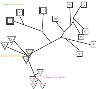
The similarities between the sound samples recorded by each DTAG were computed as described in Sec. II C, and the resulting phylogeny that visualizes the similarities is dis-played in Fig.3. As described in Sec.II B, each number is a set of whale calls recorded by a single DTAG and therefore can include calls of the whale carrying the DTAG, as well as calls of whales in close proximity to the tagged whale.

As Fig.3shows, the computer analysis identified the simi-larities between the whale populations by analyzing their sounds. The pilot whales are clustered toward the bottom of the tree, and the killer whales are at the upper part of the phy-logeny. Inside the group of killer whales, the computer analy-sis was also able to separate the Icelandic killer whales (6,7,22) and the Norwegian killer whales (8,9,10,12,13,23,24), indicating that the computer analysis could sense differences in the calls made by whales of the two locations.

The algorithm also differentiated automatically between Norwegian long-finned pilot whales (15,17,18,19) and Bahamas short-finned pilot whales (1,2,3,4), showing that these two sister species of pilot whales also recorded identifi-able differences in their calls. The Norwegian pilot whale calls were collected close to the coasts of Norway, but placed by the algorithm far from the Norwegian killer whales, showing that according to the data used in this study, the difference in acoustic repertoires of killer whales and

pilot whales is stronger than the difference in the acoustic background that can be attributed to the geographic location. This is a strong indication that the machine learning methods are driven by real differences in whale calls instead of differ-ences in acoustic background that may be location dependent.

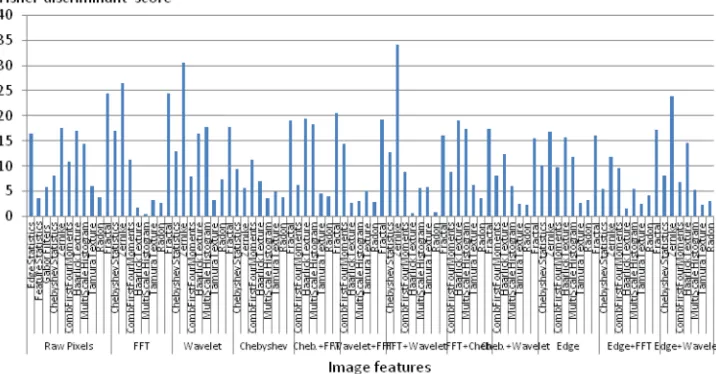
As described in Sec.II C, the analysis is based on very many content descriptors that reflect the spectrograms in a numerical fashion. These descriptors are weighted by their Fisher discriminant scores for their informativeness, and that score determines the impact of the content descriptor on the analysis so that content descriptors with a high Fisher dis-criminant score have a high impact on the results, while descriptors with low Fisher scores are assumed to be uninfor-mative and will have little or no effect on the analysis (Shamir et al., 2008a; Shamiret al., 2010a). Figure 4 dis-plays the values of the Fisher scores of the groups of features used in the analysis.

As Fig.4shows, the features with the highest Fisher dis-criminant scores are the polynomial decomposition descrip-tors such as the Chebyshev features and Zernike polynomials (Teague, 1980). Polynomial decomposition fea-tures are based on the representation of a wave using the coefficients of the polynomials that approximate it, provid-ing with an efficient mechanism to compare waves and reduce the dimensionality of the data. Another group of fea-tures that are informative is the fractal feafea-tures (Wu et al., 1992). Fractality analysis has been shown to be useful in audio analysis (Kumar and Johnson, 1993) and, in particular, analysis of waveform graphs such as speech audio (Pickover and Khorasani, 1986). As can be seen in the example Fig.2, the density and distances between the different lines in the spectrograms of killer and pilot whales can be different, and therefore the differences can be sensed by the coefficients of the polynomial decomposition. Another simple example of a feature that can differentiate between the spectrogram is the edge statistics computed from the raw pixels, as more lines in the spectrogram can be reflected by more and sharper edges.

To test the consistency of the method with different dis-tance metrics, we also tested the method so that the disdis-tances between the samples are measured using the weighted Minkowski distance such that the exponent is set to 4 as shown by

d¼

ffiffiffiffiffiffiffiffiffiffiffiffiffiffiffiffiffiffiffiffiffiffiffiffiffiffiffiffiffiffiffiffiffiffi XjXj

f¼1

WfðXfYfÞ

4 4

v u u

t : (4)

Figure 5shows the resulting graph, which is in agreement with the graph generated with the weighted Euclidean dis-tances and separates the whales into the same groups.

A. Comparison with the citizen scientists’ analysis of individual calls

As described in Sec.II A, Whale FM citizen scientists match each whale call with a set of other calls acquired by whales of the same species, but these calls are not necessar-ily recorded in the same tag deployment. In that sense, the manual analysis is different from the computer analysis in which each call is compared to all other calls, and not just calls recorded by tags deployed in whales of the same species.

Since the citizen scientists do not assign the calls with features or continuous values, it is not possible to identify features used by the citizens and the same method used in the machine learning analysis. Instead, these manual classifi-cations can be used to estimate the similarity between the calls recorded by each pair of whale tag deployments {x,y}, deduced by the number of classifications of calls recorded by the tag carried by whalexclassified by Whale FM partici-pants as most similar to a call recorded by the tag carried by whale y, and the classifications of the calls recorded by whale yas most similar to calls recorded by the tag carried by whale x. High confusion between the calls recorded in tags carried by two different whales indicates that according to the perception of Whale FM citizen scientists, the calls

acquired in these two deployments are more similar to each other compared to the other recordings.

At the time of writing, more than 10 000 volunteers have contributed more than 190 000 matches (including anti-matches) via Whale FM. Eighty-three thousand of these matches were performed by unregistered users, the remain-ing 107 000 classifications were contributed by 6458 people. Whale FM registered volunteers perform a median of 5 clas-sifications each, 200 people contributed 100 or more classifi-cations, and 8 people contributed 500 or more.

The matches in Whale FM are combined together, and the ratio of matches to anti-matches between two calls is used to determine if they are alike. In this analysis, we con-sider pairs of calls that have been independently matched more often than they are anti-matched by volunteers. The result is a set of 25 512 “cleaned” pairs of whale calls.

Based on the association of the whale calls to calls of other whales, the similarity value Sx,y between the calls of

whalexand whaleywas then computed by

Sx;y¼

1 2

xy

X

i

xi

þXyx

i

yi

0 @

1

A; (5)

wherexyis the number of whale calls of whalexclassified

by Whale FM participants as whaley, andyxis the number

of calls of whale y classified as whale x. This similarity value can be conceptualized as the mean of the number of calls of whale xidentified as whale y, divided by the total number of call classification of whale x, and the number of calls of whale yidentified as whale x, divided by the total number of call classifications of whaley.

Repeating this process for all possible pairs of whales using 25 512 human classifications of the whale calls

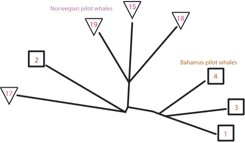
produced a similarity matrix that was visualized as a phylog-eny using the Phylip package as described in Sec.III. Since all citizen scientist classifications were by matching target calls to calls made by whales of the same species, the analy-sis of the manual classifications was separated to killer and pilot whales. Figures 6 and 7 display the phylogenies that visualize the citizen scientist classifications of the killer and pilot whales, respectively.

As Fig.6shows, the analysis of the classifications of the citizen scientists shows separation between Norwegian and Icelandic killer whales, indicating that the human partici-pants preferred to match the target calls with calls recorded by tags carried by whales of the same geographical location, even if the calls were not recorded in the same tag deploy-ment. Figure 7 also shows separation between Bahamas short-finned and Norwegian long-finned pilot whales. However, the analysis of the citizen scientists placed the calls recorded by whale 2 in the Bahamas close to the

FIG. 5. (Color online) The evolution-ary tree created automatically when using Minkowski distances instead of the weighted Euclidean distances.

Norwegian pilot whales, indicating that the citizen scientists found it difficult to differentiate between these calls and the calls recorded by the tags carried by whales 15, 17, 18, and 19. It is important to note that the manual analysis of a single volunteer can only compare a whale call to a limited number of other calls, and therefore the citizen scientists could only match a call with the most similar call within a subset, while the faster computer analysis compared each call to all other whale calls in the dataset, and therefore could find more sim-ilar matches leading to a more accurate analysis.

IV. CONCLUSION

The purpose of this study was to demonstrate two meth-ods for analyzing large acoustic datasets, and study differen-ces between sounds of different species or subpopulations of whales. First, a method that can automatically identify and analyze whale calls is developed and tested. This method is compared to human perception of killer whale and pilot whale sounds, which is based on classifications performed by over 10 000 volunteers in the Whale FM citizen science project. Unlike previous machine learning studies of whale sounds, the acoustic characteristics being measured were automatically determined by their information content instead of being selected by scientists.

Although we use Fisher discriminant scores to weigh the features, the features are weighted by their ability to dif-ferentiate between whales, and not by their ability to differ-entiate between the groups of whales. The only knowledge used by the algorithm is that there are different whales in the dataset, but no annotation of the species or geographical locations of the whales is used at any point, and the algo-rithm finds the structure and separates the whales into the different groups automatically and without any prior knowl-edge about the nature or existence of such groups in the data. Our experimental results show that the machine percep-tion is sensitive to the different calls of whales, and the method was able to correctly separate the dataset of whales into different species and populations in an unsupervised fashion. The results also show that data taken from manual classification of the sounds performed by citizen scientists also provided an informative analysis, despite the fact that the citizen scientists were asked to identify calls, and not

individual whales or species. Citizen science analysis and computer methods are likely to be used in the future for fur-ther analysis of large datasets of whale sounds for the pur-pose of profiling the way whales communicate.

Both computer and human analysis show sound differen-ces between Norwegian and Icelandic killer whales, and also between Norwegian long-finned and Bahamas short-finned pilot whales. The ability of the system to classify between whale calls can be attributed to differences in the audio sys-tems that were used to acquire the sounds. However, the main purpose of the paper is not to classify between whales, but to measure the similarities between the calls of whales and char-acterize the similarities in an unsupervised fashion. The unsu-pervised analysis of the similarities is more informative compared to merely measuring the classification accuracy into one of a discrete set of whale call classes, and is therefore less sensitive to false positives due to differences between the audio acquisition systems. For instance, all Bahamas pilot whales are placed closer to all Norwegian pilot whales, and are more distant from the killer whales. A possible bias caused by geographic location is rejected by the observation that the audio from different sites in the same geographic location are similar to each other when recording the sounds of the same species, but are very different when recording the sounds of whales of different species, as the Norwegian killer whales and Norwegian pilot whales are positioned in distant areas in the phylogeny. Also, the sounds of the Norwegian killer whales were acquired in two different years (2005 and 2006), but still the Norwegian killer whales are positioned on the same branch in the phylogeny, showing that the sounds are not separated by the audio acquisition campaign. Another example is the Norwegian pilot whale data, which were also collected in two different years (2008 and 2009), and are still grouped very close to each other in the phylogeny.

ACKNOWLEDGMENTS

Zooniverse is supported by NSF Grant No. 0941610. We gratefully acknowledge help from data collectors: Ari Shapiro, Laela Sayigh, Ricardo Antunes, and Ana Catarina Alves. Acoustic data were collected as part of the BRS and 3S behavioral response studies. We thank all Whale FM vol-unteers who helped matching data (a full list of contributing volunteers can be found at http://whale.fm/contributors). Further, we gratefully acknowledge Scientific American for supporting the Whale FM project. A.M.v.B.B. acknowledges support from the Sea Mammal Research Unit at the University of St. Andrews (Professor Ian Boyd) and Woods Hole Oceanographic Institution for the Whale FM project. The computing cluster that processed the data was funded by NSF Grant No. 1157162. P.T. received funding from the Marine Alliance for Science and Technology for Scotland (MASTS) and their support is gratefully acknowledged. MASTS is funded by the Scottish Funding Council (grant HR09011) and contributing institutions.

Barlow, H. B. (1989). “Unsupervised learning,” Neural Comput.1, 295–311. Barrett-Lennard, L. G., Ford, J. K. B., and Heise, K. A. (1996). “The mixed

blessing of echolocation: Differences in sonar use by fish-eating and mammal-eating killer whales,” Anim. Behav.51, 553–566.

Bishop, C. M. (2006). Pattern Recognition and Machine Learning

(Springer, New York), pp. 191–192.

Deecke, V. B., Ford, J. K. B., and Spong, P. (1999). “Quantifying complex patterns of bioacoustic variation: Use of a neural network to compare killer whale (Orcinus orca) dialects,” J. Acoust. Soc. Am.105, 2499–2507. Felsenstein, M. (2004). “PHYLIP phylogeny inference package,” Version

36, 2004 (2004).

Fischer, D., Schwamb, M., Schawinski, K., Lintott, C., Brewer, J., Giguere, M., Lynn, S., Parrish, M., Sartori, T., Simpson, R., Smith, A., Spronck, J., Batalha, N., Rowe, J., Jenkins, J., Bryson, S., Prsa, A., Tenenbaum, P., Crepp, J., Morton, T., Howard, A., Beleu, M., Kaplan, Z., vanNispen, N., Sharzer, C., DeFouw, J., Hajduk, A., Neal, J., Nemec, A., Schuepbach, N., and Zimmermann, V. (2012). “Planet Hunters: The first two planet candi-dates identified by the public using the Kepler Public Archive Data,” Mon. Not. R. Astron. Soc.419, 2900–2911.

Ford, J. K. B. (1989). “Acoustic behavior of resident killer whales (Orcinus orca) off Vancouver Island, British Columbia,” Can. J. Zool.67, 727–745. Ford, J. K. B., Ellis, G. M., and Balcomb, K. C. (2000).Killer whales: The Natural History and Genealogy of Orcinus orca in British Columbia and Washington, 2nd ed. (University of British Columbia Press, Vancouver), pp. 1–104.

Glotin, H., Caudal, F., and Giraudet, P. (2008). “Whales cocktail party: A real-time tracking of multiple whales,” Int. J. Can. Acoust.36, 141–147 (2008).

Johnson, M. P., and Tyack, P. L. (2003). “A digital acoustic recording tag for measuring the response of wild marine mammals to sound,” IEEE J. Ocean. Eng.28, 3–12.

Kumar, A. R., and Johnson. D. H. (1993). “Analyzing and modeling fractal intensity point processes,” J. Acoust. Soc. Am.93, 3365–3373.

Lintott, C., Schawinski, K., Bamford, S., Slosar, A., Land, K., Thomas, D., Edmondson, E., Masters, K., Nichol, R., Raddick, M. J., Szalay, A., Andreescu, D., Murray, P., and van den Berg, J. (2011). “Galaxy zoo 1: Data release of morphological classifications for nearly 900,000 galaxies,” Mon. Not. R. Astron. Soc.410, 166–178.

Lintott, C., Schawinski, K., Slosar, A., Land, K., Bamford, S., Thomas, D., Raddick, M. J., Nichol, R., Szalay, A., Andreescu, D., Murray, P., and van den Berg, J. (2008). “Galaxy zoo: Morphologies derived from visual inspection of galaxies from the Sloan Digital Sky Survey,” Mon. Not. R. Astron. Soc.389, 1179–1189.

Miller, P. J. O. (2006). “Diversity in sound pressure levels and estimated active space of resident killer whale vocalizations,” J. Comp. Physiol., A

192, 449–459.

Miller, P. J. O., and Bain, D. E. (2000). “Within-pod variation in the sound production of a pod of killer whales,Orcinus orca,” Anim. Behav. 60, 617–628.

Miller, P. J. O., Kvadsheim, P., Lam, F. P. A., Wensveen, P. J., Antunes, R., Alves, A. C., Visser, F., Kleivane, L., Tyack, P. L., and Doksæter Sivle, L. (2012). “The severity of behavioral changes observed during experimental exposures of killer (Orcinus orca), long-finned pilot (Globicephala melas), and sperm whales (Physeter macrocephalus) to naval sonar,” Aquat. Mamm.38, 362–401.

Miller, P. J. O., Shapiro, A. D., Tyack, P. L., and Solow, A. R. (2004) “Call-type matching in vocal exchanges of free-ranging resident killer whales

Orcinus orca,” Anim. Behav.67, 1099–1107.

Nousek, A. E., Slater, P. J. B., Wang, C., and Miller, P. J. O. (2006). “The influence of social affiliation on individual vocal signatures of northern resident killer whales (Orcinus orca),” Biol. Lett.2, 481–484.

Oswald, J. N., Barlow, J., and Norris, T. F. (2003). “Acoustic identification of nine delphinid species in the eastern tropical Pacific Ocean,” Marine Mammal Science19, 20–37.

Ottensmeyer, C. A., and Whitehead, H. (2003). “Behavioural evidence for social units in long-finned pilot whales,” Can. J. Zool.81, 1327–1338. Pickover, C. A., and Khorasani, A. (1986). “Fractal characterization of

speech waveform graphs,” Comput. Graph.10, 51–61.

Riesch, R., and Deecke, V. (2011). “Whistle communication in mammal-eating killer whales (Orcinus orca): Further evidence for

acoustic divergence between ecotypes,” Behav. Ecol. Sociobiol. 65, 1377–1387

Riesch, R., Ford, J. K. B., and Thomsen, F. (2006). “Stability and group specificity of stereotyped whistles in resident killer whales,Orcinus orca, off British Columbia,” Anim. Behav.71, 79–91.

Samarra, F. I. P., Deecke, V. B., Vinding, K., Rasmussen, M. H., Swift, R. J., and Miller, P. J. O. (2010). “Killer whales (Orcinus orca) produce ultrasonic whistles,” J. Acoust. Soc. Am.128, EL205–EL210.

Sayigh, L., Quick, N., Hastile, G., and Tyack, P. (2013). “Repeated call types in short-finned pilot whales,Globicephala macrorhynchus,” Marine Mammal Sci.29, 312–324.

Schevill, W. E., and Watkins, W. A. (1966). “Sound structure and direction-ality inOrcinus(killer whale),” Zoologica (N.Y.)51, 71–76.

Shamir, L. (2009). “Automatic morphological classification of galaxy images,” Mon. Not. R. Astron. Soc.399, 1367–1372.

Shamir, L., Delaney, J., Orlov, N., Eckley, D. M., and Goldberg, I. G. (2010b). “Pattern recognition software and techniques for biological image analysis,” PLoS Comput. Biol.6, e1000974.

Shamir, L., Ling, S., Rahimi, S., Ferrucci, L., and Goldberg, I. (2009a) “Biometric identification using knee X-rays,” Biometrics1, 365–370. Shamir, L., Ling, S. M., Scott, W., Boss, A., Orlov, N., Macura, T., Eckley,

D. M., Ferrucci, L., and Goldberg, I. G. (2009b). “Knee X-ray image anal-ysis method for automated detection of Osteoarthritis,” IEEE Trans. Biomed. Eng.56, 407–415.

Shamir, L., Macura, T., Orlov, N., Eckley, D. M., and Goldberg, I. G. (2010a). “Impressionism, expressionism, surrealism: Automated recogni-tion of painters and schools of art,” ACM Trans. Appl. Percept.7(2), 1. Shamir, L., Orlov, N., Eckley, D. M., Macura, T., and Goldberg, I. G.

(2008b). “IICBU 2008—A proposed benchmark suite for biological image analysis,” Med. Bio. Eng. Comp.46, 943–947.

Shamir, L., Orlov, N. D., Eckley, M., Macura, T., Johnston, J., and Goldberg, I. G. (2008a). “Wndchrm—An open source utility for biological image analysis,” Source Code Biol. Med.3, 13.

Shamir, L., and Tarakhovsky, J. (2012). “Computer analysis of art,” ACM J. Comput. Cultural Heritage5(2), 7.

Simpson, R., Povich, M., Kendrew, S., Lintott, C., Bressert, E., Arvidsson, K., Cyganowski, C., Maddison, S., Schawinski, K., Sherman, R., Smith, A., and Wolf-Chase, G. (2012). “The Milky Way Project first data release: A bubblier galactic disc,” Mon. Not. R. Astron. Soc.424, 2442–2460. Svatora, S., and Shamir, L. (2012). “Improving Eastern Bluebird nest box

performance using computer analysis of satellite images,” Comput. Ecol. Software2, 96–102.

Teague M. (1980). “Image analysis via the general theory of moments,” J. Opt. Soc. Am.70, 920–930.

Thomsen, F., Franck, D., and Ford, K. B. (2002). “On the communicative significance of whistles in wild killer whales (Orcinus orca),” Naturwissenschaften89, 404–407.

Tyack, P. L., Johnson, M., Aguilar, N., Sturlese, A., and Madsen, P. (2006). “Extreme diving of beaked whales,” J. Exp. Biol.209, 4238–4253. Tzanetakis, G., and Cook, P. (2002). “Musical genre classification of audio

signals,” IEEE Trans. Speech Audio Process.10, 293–302.

van Parijs, S. M., Clark, C. W., Sousa-Lima, R. S., Parks, S. E., Rankin, S., Risch, D., and Van Opzeeland, I. C. (2009). “Management and research applications of real-time and archival passive acoustic sensors over varying temporal and spatial scales,” Mar. Ecol.: Prog. Ser.395, 21–36 (2009).

von Benda-Beckmann, A. M., Lam, F. P. A., Moretti, D. J., Fulkerson, K., Ainslie, M. A., van IJsselmuide, S. P., Theriault, J., and Beerens, S. P. (2010). “Detection of Blainville’s beaked whales with towed arrays,” Appl. Acoust.71, 1027–1035.

Wu, C. M., Chen, Y. C., and Hsieh, K. S. (1992). “Texture features for clas-sification of ultrasonic liver images,” IEEE Trans. Med. Imaging 11, 141–152.