Impacts of sample design for validation data on the accuracy of feedforward neural network classification

sciences

Article

Impacts of Sample Design for Validation Data on the

Accuracy of Feedforward Neural

Network Classification

Giles M. Foody ID

School of Geography, University of Nottingham, University Park, Nottingham NG7 2RD, UK; [email protected]; Tel.: +44-115-951-5430

Received: 20 July 2017; Accepted: 21 August 2017; Published: 30 August 2017

Abstract:Validation data are often used to evaluate the performance of a trained neural network and used in the selection of a network deemed optimal for the task at-hand. Optimality is commonly assessed with a measure, such as overall classification accuracy. The latter is often calculated directly from a confusion matrix showing the counts of cases in the validation set with particular labelling properties. The sample design used to form the validation set can, however, influence the estimated magnitude of the accuracy. Commonly, the validation set is formed with a stratified sample to give balanced classes, but also via random sampling, which reflects class abundance. It is suggested that if the ultimate aim is to accurately classify a dataset in which the classes do vary in abundance, a validation set formed via random, rather than stratified, sampling is preferred. This is illustrated with the classification of simulated and remotely-sensed datasets. With both datasets, statistically significant differences in the accuracy with which the data could be classified arose from the use of validation sets formed via random and stratified sampling (z= 2.7 and 1.9 for the simulated and real datasets respectively, for bothp< 0.05%). The accuracy of the classifications that used a stratified sample in validation were smaller, a result of cases of an abundant class being commissioned into a rarer class. Simple means to address the issue are suggested.

Keywords: cross-validation; multi-layer perceptron; remote sensing; classification error; sample design; machine learning

1. Introduction

Artificial neural networks are widely used for supervised classification applications. In these applications, cases of known class membership are used to train the neural network in order to allow it to predict the class membership of previously unseen and unlabeled cases. This type of analysis is common in, for example, the production of thematic maps, such as those depicting land cover, from remotely-sensed imagery [1–3]. The imagery contain data on the remotely-sensed response of the land surface that is converted into information on land cover class via the classification analysis and a wide variety of approaches and applications have been investigated, e.g., [2,4,5]. Neural networks have become a popular method for image classification as numerous studies have shown that they can yield more accurate maps than a variety of other alternative approaches to classification [6–8]. The relative performance of neural network classifiers in relation to a range of alternative methods, including standard statistical classifiers, machine learning methods, and decision trees, is discussed in the literature (e.g., [1]). As with all classifiers, the quality of the final classification is, however, in part a function of the classifier and the nature, notably the size and quality, of the ground reference dataset on the class membership used [9–12]. Ground reference data are used to provide data to train the neural network and to evaluate the quality of its predictions. The latter is typically expressed in terms of the overall accuracy of the classification output from the network.

Appl. Sci.2017,7, 888 2 of 15

In remote sensing applications, the class membership of the cases in the training set is typically determined by ground-based observation or interpretation of very fine spatial resolution imagery [1,13]. Clearly, the nature and quality of the ground reference data used will impact upon the accuracy of the predictions obtained from the neural network. Classification accuracy is, for example, influenced by the size, composition, and quality of the ground reference dataset used in training [2,9,10,14–16]. The way the ground reference data are used is also important, especially if part of it is used for the purpose of validation [10]. The use of some reference data for validation purposes, to indicate the quality of the trained model generated, is commonplace in defining a supposedly optimal neural network. In common remote sensing applications, the optimal approach would be the one that yielded the most accurate thematic map when applied to the image data.

In a typical remote sensing application, the aim of the classification is to accurately map the land cover classes in the region of study. Throughout there are a set of basic assumptions made in classification analyses. These include the need for the set of classes to be mutually exclusive and exhaustively defined. Failure to satisfy these assumptions will result in errors. Cases of an untrained class will, for example, typically have to be allocated erroneously to one of the defined classes [17]. Although there are instances when a neural network may be used to obtain a non-standard classification, such as soft classification when classes intergrade or are mixed together [17], the standard hard classification in which a case belongs fully to a single class is the focus on this article. In all cases, the ground reference data used in training, validating, and testing the neural network have a key role to play in the production of an accurate map. Hence, the design of these datasets is important.

Good practices for classification accuracy assessment for the evaluation of the quality of thematic maps derived via remote sensing have been defined and include guidance on the construction of the testing sample upon which the assessment is to be based. Typically, for example, the use of a reference dataset acquired following a probabilistic sampling design is recommended [18,19]. This allows a rigorous design-based assessment of classification accuracy, typically based upon the analysis of an error or confusion matrix in which the predicted class label obtained from the neural network is cross-tabulated against the label in the reference dataset for the sample of cases under consideration [1,18].

The goal of training a classifier is different to that of testing its output predictions and, hence, the nature of the ideal training set may be very different to that of the testing set. In training, the aim is, essentially, to guide the neural network to learn the identity of the classes from their remotely-sensed response. Thus, the observed remotely-sensed response for the training sample of known class membership is used in network learning to ultimately form decision rules to accurately label cases of unknown class membership in order to map the region of interest [1]. Much conventional guidance on the design of the training set in remote sensing applications is based upon historical work undertaken with conventional statistical classifiers, such as the maximum likelihood classification. This advice typically calls for the sample size to be estimated following basic sampling theory in order to derive a representative and unbiased description of each class to allow cases of unknown class membership to then be allocated the label of the class they had greatest similarity to. Alternatively, a simple heuristic, such as the use of a sample of cases for each class, the size of which is at least 10 times the number of discriminating variables, such as the spectral wavebands, are used [10,20,21]. In essence, this type of approach is calling for the use of a stratified sample design in the formation of the training set. Despite the development of new classifiers, such approaches are still widely used even though the nature of the ideal training set varies between classifiers.

require only a small number of training cases, but these are anti-boundary in nature [12]. Considerable research has, therefore, focused on how the properties of the training dataset impact on a classification, typically with a desire to maximize the final mapping accuracy (e.g., [9,10,24–26]). Sometimes it may be possible to predict the location of useful candidate training cases for a classification [27] or, contrary to conventional approaches, even deliberately use mixed cases in training and the analyst can seek to form a training set intelligently for a given application scenario [22,28,29]. As such, there is no single ideal way to define a training set that is universally applicable. Given the popularity of consensus or ensemble methods that use a variety of different classifiers [7,30] it is common to see relatively large training sets acquired following conventional guidance. While this approach may sometimes be inefficient, notably in that the sample may be larger than needed, it has the capacity to provide useful training data for a wide range of classifiers. It is, therefore, common to see either a training sample designed explicitly for a specific task, which could be a small and highly unrepresentative sample [29,31], or the use of a stratified design that seeks to ensure each class can be described well [1]. The design details are, however, important. The nature of the training set has a significant impact on the accuracy of predictions by a neural network [2,15,32]. For example, the size of the training set, notably in relation to the complexity of the network, can have a marked effect on classification by a neural network [9,16,33]. The composition of the training set in terms of relative class abundance is also important [15,34]. Variations in class abundance can yield imbalanced datasets that, as in other classifiers, can have substantial impacts on the final classification.

Appl. Sci.2017,7, 888 4 of 15

The composition of the sample of cases forming the validation set, notably in terms of the relative abundance of the cases of the classes may vary as a function of the design used to acquire the training dataset. If the validation sample is formed with a simple random sample design it is likely to be imbalanced in composition, with the number of cases of a class reflecting its relative abundance in the region being mapped. The use of a stratified sample design in the generation of the validation sample will act to give a balanced dataset but this need not be an ideal approach. Indeed, the use of a stratified design could result in the selection of a network that was sub-optimal for the task if the classes vary in abundance and separability. For example, standard approaches to the assessment of overall classification accuracy weight errors equally and could inflate the importance of rare classes while deflating that of abundant classes. Sometimes it may be possible to account for the sample design if there is information on class abundance [18]. Alternatively, if the study aim is focused on a single class, which is often the case, the accuracy assessment used in the validation could be focused on that class at the expense of the others. However, for a general purpose map, it may be more appropriate to follow the guidance on sampling that is typically used in the formation of the testing set as this typically allows for variations in class abundance to be accounted for.

The effect of different sample designs for the formation of the validation dataset is explored in this paper. Specifically, the focus is on the use of samples acquired by simple random and stratified random sampling designs (both without replication). Due to the way overall accuracy is typically estimated with a validation sample, it is hypothesized that the overall accuracy of the final classification, evaluated using the testing set, will be larger for a neural network trained using a validation sample generated via simple random as opposed to stratified random sampling. Indeed a series of outcomes may be predicted as having the potential to arise as a function of the validation dataset used. For example, in relation to two classes that overlap, it would be expected that the hyperplane to best separate the classes fitted when a balanced validation set was used would migrate away from the more abundant class if an imbalanced training set was used. As a consequence of this, there is an opportunity for the accuracy with which the more abundant class is classified to rise as fewer cases of it will be omitted from it and fewer of its cases commissioned by the rarer class (es). These trends arise as classification errors are weighted equally in standard assessments of overall accuracy. The overall trend expected would be for the accuracy with which the abundant class is classified to increase while the accuracy of the classification of the rarer class would decline. As such it is hypothesized that the use of a stratified sample design may not be ideal as its use relative to a randomly-defined validation dataset would be associated with a decrease in overall accuracy, arising noticeably through a decrease in the accuracy for the abundant class (es) as a result of an increase in the commission of cases of abundant class (es) by the set of rarer classes.

2. Data and Methods

Two datasets were used. First, a simulated dataset was used to illustrate the issues and also to facilitate, if desired, replication. Second, a real dataset consisting of remotely-sensed data and associated ground reference data on land cover class labels was used.

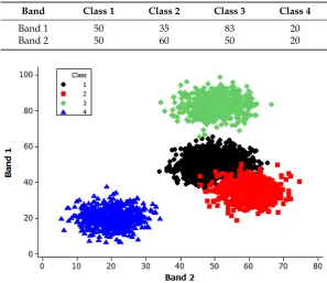
A very simple multi-class classification scenario was simulated. This comprised data on four classes acquired in two dimensions, or bands. The data for each class were formed using a random number generator using analyst provided values for the class mean and standard deviation on the assumption that the data for each class were normally distributed. For each class the standard deviation was set equal to 5 and the mean values used to generate the data in each band are shown in Table1. In the scenario generated, class 1 was the most abundant class. Specifically, class 1 was five times more abundant than each of the other classes. Most attention was focused on class 1 and class 2, which exhibited a degree of overlap in their distributions with class 3 and, especially, class 4 was highly separable (Figure1).

random sampling and the other formed via a stratified random sample design. In brief, a single training set was generated using a stratified random sample of 400 cases per-class. Similarly, a single testing set was used to evaluate the accuracy of the classifications from the neural networks selected as optimal in each series of analyses undertaken. This testing set was simulated to represent a sample acquired by simple random sampling and comprised 800 cases. Due to the way the scenario was designed, class 1 was five times more abundant in it than the other classes. The two validation datasets used each contained 800 cases, but one was formed via a simple random sample in which class abundance varied as in the testing set, while the other was formed with a stratified random sample in which each class was equally represented. Each series of neural network analyses used a software package that sought to generate an optimal network, with optimality defined as the maximization of the overall accuracy with which the validation set was classified.

The remotely-sensed data were acquired by an airborne thematic mapper (ATM) sensor for a test site near the village of Feltwell, Norfolk, UK. The latter is located approximately 58 km to the northeast of the city of Cambridge. The land around the village was topographically flat and its land cover mosaic was characterized mainly by large agricultural fields. At the time of the ATM data acquisition these fields had also typically been planted with a single crop type (Figure2).

The ATM used was a basic multispectral scanning system that acquired data in 11 spectral wavebands from blue to thermal infrared wavelengths (Table3). Given the relatively low altitude of airborne data acquisition (~2000 m), the spatial resolution of the imagery was very much smaller than the typical field size, approximately 5 m. As a result, image pixels tended to represent an area composed of a single class (i.e., pure pixels) and, hence, were appropriate for hard image classification analysis; boundary pixels were ignored. Attention focused here on the six crop classes that dominated the region at the time of the ATM data acquisition. These classes and their approximate coverage (%) of the study area at the time were: sugar beet (S, 30.3%), wheat (W, 30.0%), barley (B, 16.0%), carrot (C, 10.3%), potato (P, 7.8%), and grass (G, 5.4%).

Table 1.The classes in the simulated dataset; note: units are arbitrary.

Band Class 1 Class 2 Class 3 Class 4

Band 1 50 35 83 20

Band 2 50 60 50 20

Appl. Sci. 2017, 7, 888 5 of 15

datasets used each contained 800 cases, but one was formed via a simple random sample in which class abundance varied as in the testing set, while the other was formed with a stratified random sample in which each class was equally represented. Each series of neural network analyses used a software package that sought to generate an optimal network, with optimality defined as the maximization of the overall accuracy with which the validation set was classified.

The remotely-sensed data were acquired by an airborne thematic mapper (ATM) sensor for a test site near the village of Feltwell, Norfolk, UK. The latter is located approximately 58 km to the northeast of the city of Cambridge. The land around the village was topographically flat and its land cover mosaic was characterized mainly by large agricultural fields. At the time of the ATM data acquisition these fields had also typically been planted with a single crop type (Figure 2).

The ATM used was a basic multispectral scanning system that acquired data in 11 spectral wavebands from blue to thermal infrared wavelengths (Table 3). Given the relatively low altitude of airborne data acquisition (~2000 m), the spatial resolution of the imagery was very much smaller than the typical field size, approximately 5 m. As a result, image pixels tended to represent an area composed of a single class (i.e., pure pixels) and, hence, were appropriate for hard image classification analysis; boundary pixels were ignored. Attention focused here on the six crop classes that dominated the region at the time of the ATM data acquisition. These classes and their approximate coverage (%) of the study area at the time were: sugar beet (S, 30.3%), wheat (W, 30.0%), barley (B, 16.0%), carrot (C, 10.3%), potato (P, 7.8%), and grass (G, 5.4%).

Table 1. The classes in the simulated dataset; note: units are arbitrary.

Band Class 1 Class 2 Class 3 Class 4

Band 1 50 35 83 20

Band 2 50 60 50 20

Figure 1. Simulated data (training, validation (random), and testing). Note: class 2 is shown overlaid on top of part of class 1 and the area of overlap may be inferred.

Appl. Sci.Appl. Sci. 20172017, ,77, 888, 888 6 of 15 6 of 15

(a) (b) (c)

Figure 2. Data for Feltwell. (a) The location of Feltwell, © OpenStreetMap contributors; (b) airborne thematic mapper (ATM) image extract in waveband 4 and (c) ATM image extract in waveband 7.

Table 2. Class composition of the datasets used for analyses of the simulated data.

Dataset Size and Class Composition

Training 400 cases of each class; total = 1600 cases

Validation (random)

500 class 1 100 class 2 100 class 3

100 class 4; total = 800 cases Validation (stratified) 200 cases of each class; total = 800 cases

Testing

500 class 1 100 class 2 100 class 3

100 class 4; total = 800 cases

Table 3. The 11 spectral wavebands of the ATM sensor used.

Waveband Wavelength (µm)

1 0.42–0.45 2 0.45–0.52 3 0.52–0.60 4 0.60–0.63 5 0.63–0.69 6 0.69–0.75 7 0.76–0.90 8 0.91–1.05 9 1.55–1.75 10 2.08–2.35 11 8.50–13.00

Ground reference data for the purposes of network learning (training) and evaluation were acquired. Following [43,44], the ground reference dataset was partitioned such that 50% was used for training, 25% for validation, and 25% for testing. The composition of these datasets, however, sometimes varied (Table 4).

Conventional guidance on the design of the training set was followed with 110 cases of each class obtained for training purposes; meeting the often stated requirement of a sample of at least 10

Figure 2.Data for Feltwell. (a) The location of Feltwell, © OpenStreetMap contributors; (b) airborne thematic mapper (ATM) image extract in waveband 4 and (c) ATM image extract in waveband 7.

Table 2.Class composition of the datasets used for analyses of the simulated data.

Dataset Size and Class Composition

Training 400 cases of each class; total = 1600 cases

Validation (random)

500 class 1 100 class 2 100 class 3

100 class 4; total = 800 cases

Validation (stratified) 200 cases of each class; total = 800 cases

Testing

500 class 1 100 class 2 100 class 3

100 class 4; total = 800 cases

Table 3.The 11 spectral wavebands of the ATM sensor used.

Waveband Wavelength (µm)

1 0.42–0.45

2 0.45–0.52

3 0.52–0.60

4 0.60–0.63

5 0.63–0.69

6 0.69–0.75

7 0.76–0.90

8 0.91–1.05

9 1.55–1.75

10 2.08–2.35

11 8.50–13.00

Ground reference data for the purposes of network learning (training) and evaluation were acquired. Following [43,44], the ground reference dataset was partitioned such that 50% was used for training, 25% for validation, and 25% for testing. The composition of these datasets, however, sometimes varied (Table4).

number of discriminating variables (wavebands) used as input. The training set, therefore, contained 660 cases acquired by a stratified random sampling design. This training set was used throughout.

Testing sets should, ideally, be acquired using a probability sampling design [18,19]. Here, a simple random sample (without replication) was used to acquire 330 cases to use for testing. Note that this sample size exceeds that required for accuracy estimation of a map with an accuracy of 85%, a standard if contentious target accuracy in remote sensing, with an allowable error of 4%. This testing set was used in all analyses of the ATM data. This latter issue impacts on comparisons of accuracy estimates and requires the use of a technique suited for related samples [45].

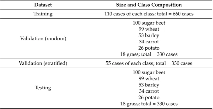
Table 4.Class composition of the datasets used for analyses of the remotely sensed data.

Dataset Size and Class Composition

Training 110 cases of each class; total = 660 cases

Validation (random)

100 sugar beet 99 wheat 53 barley 34 carrot 26 potato 18 grass; total = 330 cases

Validation (stratified) 55 cases of each class; total = 330 cases

Testing

100 sugar beet 99 wheat 53 barley 34 carrot 26 potato 18 grass; total = 330 cases

As with the analyses of the simulated dataset, the search for an optimal neural network was undertaken twice. In each case the training and testing sets were the same, the only difference was the composition of the validation set used to identify the optimal network from a set of candidate networks generated for the task. In one set of analyses, the validation set was generated by simple random sampling and thus the number of cases of each class tended to reflect the actual abundance of the classes in the region to be mapped. Indeed, here, the sample was selected to ensure that the class composition of the validation set equalled that of the testing set. This sample comprised 330 cases. In the other set of analyses, a validation sample of the same size, but acquired following a stratified random sample such that each class was equally represented was used. The nature of the datasets used is summarized in Table4.

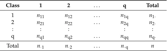
In the search for an optimal neural network to classify the ATM data, optimality was defined in relation to the maximum overall accuracy of the classification of the validation data. The accuracy of each classification was calculated from the confusion or error matrix generated for it which shows a cross-tabulation predicted and actual class label for each case in the dataset analysed [1,18]. Using the layout and notation defined for the confusion matrix shown in Table5, which is used throughout the article, overall accuracy,O, was calculated using Equation (1):

O= ∑nii

n (1)

In addition to the global estimate of classification quality conveyed by overall accuracy, the producer’s,P, and user’s accuracy,U, were calculated with reference to each class [1,18]. These were obtained for classifrom Equations (2) and (3) respectively:

Pi = nii

Appl. Sci.2017,7, 888 8 of 15

Ui= nii

ni· (3)

Note that, as is common, the calculations of these measures of accuracy are based on the raw counts of cases shown in the elements of the confusion matrix. These approaches to accuracy assessment were used to support all analyses, whether based on the training, validation, or testing datasets. Most focus is, however, on the accuracy values arising from analyses of the validation and testing datasets.

To determine if the use of different validation samples impacted on the accuracy of the final thematic classification, the statistical significance of differences in the accuracy of the classifications of the testing set were assessed. Standard approaches for the comparison of accuracy values that are popular in remote sensing projects are unsuitable here as the same sample of testing cases was used throughout. To accommodate for this situation, the statistical significance of differences in accuracy was assessed using the McNemar test [45,46]. The latter is a non-parametric test that is based on a binary confusion matrix which shows the cross-tabulation of the cases that have been labelled correctly and incorrectly by the two classifications being compared. The test focuses on the discordant cases, those which were classified correctly by one classifier, but incorrectly by the other. Without continuity correction, the test is based on the normal curve deviate,z, as expressed as:

z= √nCI−nIC nCI+nIC

(4)

wherenCI indicates the number of cases in the relevant element of the matrix with the subscript Cindicating if the classification was correct in its labelling orIif it was incorrect and order of the subscripts indicates the specific classification from the pair under study. For a standard two-tailed test at the 95% level of confidence, the null hypothesis of no significant difference is rejected if the calculatedzexceeds the critical value of |1.96|. Similarly, for a one-tailed test, if the hypothesis under test has a directional component, the direction (sign) needs consideration and the magnitude of the critical value ofzto indicate that a significant difference exists at the 95% level of confidence is 1.645.

Table 5.The confusion matrix based on raw counts of cases for a classification of q classes. Matrix columns show the label in the reference data and rows the label in the classification.

Class 1 2 . . . q Total

1 n11 n12 . . . n1q n1·

2 n21 n22 . . . n2q n2·

: : : : :

q nq1 nq2 . . . nqq nq·

Total n·1 n·2 . . . n·q n

3. Results and Discussion

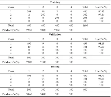
With the simulated dataset, two sets of analyses were undertaken to identify optimal neural networks, one using the validation set formed via simple random sampling and the other formed using a stratified random sample. The key properties of the selected networks and their ability to classify the datasets are defined in Table6with a full set of confusion matrices for each set of analyses shown in Tables7and8.

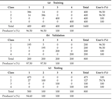
Note, for example, that relative to the classification obtained with a stratified validation sample, the use of the validation set formed by random sampling resulted in a higher overall accuracy of the testing set. This arose because of a higher accuracy with which the abundant class was classified due to a reduction in omission error (from 27 to 7 cases) and the accuracy of the rarer class it was confused with declined (Tables7and8). Critically, the results suggest that the use of a balanced training set acquired via a stratified random sample may produce a sub-optimal final output. As hypothesized, the use of a stratified sample resulted in a lower accuracy than was achievable because the accuracy with which the abundant class was classified declined, associated with a large omission error due to cases being commissioned into a rarer class.

A series of analyses was undertaken to define an optimal neural network using the two validation datasets in the analyses of the remote sensing data. The core focus here is on the classification results from the network determined to be optimal from each series of analyses. Although the precise details of the neural networks are relatively unimportant as the classifications that arise from them are the focus of attention, key details on the networks selected are summarized in Table10and the confusion matrices for the testing set are shown in Tables11and12.

Table 6. Key characteristics of the networks selected for the analyses of the simulated data; note: network architecture is expressed as input:hidden:output.

Validation

Dataset Architecture

Algorithm and Iterations

Classification Accuracy (%) Training Validation Testing

Random 2:15:2 Backpropagation 48 97.25 97.62 98.37

Stratified 2:8:2 Conjugate gradient 55 98.25 98.75 96.62

Table 7.Confusion matrices for the network selected using a validation set formed by random sampling.

Training

Class 1 2 3 4 Total User’s (%)

1 398 40 2 0 440 90.45

2 2 360 0 0 362 99.44

3 0 0 398 0 398 100

4 0 0 0 400 400 100

Total 400 400 400 400 1600

Producer’s (%) 99.50 90.00 99.50 100

Validation

Class 1 2 3 4 Total User’s (%)

1 490 9 0 0 499 98.19

2 10 91 0 0 101 90.09

3 0 0 100 0 100 100

4 0 0 0 100 100 100

Total 500 100 100 100 800

Producer’s (%) 99.00 91.00 100 100

Testing

Class 1 2 3 4 Total User’s (%)

1 493 6 0 0 499 98.79

2 7 94 0 0 101 93.06

3 0 0 100 0 100 100

4 0 0 0 100 100 100

Total 500 100 100 100 800

Appl. Sci.2017,7, 888 10 of 15

Table 8.Confusion matrices for the network selected using a validation set formed by stratified sampling.

(a) Training

Class 1 2 3 4 Total User’s (%)

1 386 14 0 0 400 96.50

2 14 386 0 0 400 96.50

3 0 0 400 0 400 100

4 0 0 0 400 400 100

Total 400 400 400 400 1600

Producer’s (%) 96.50 96.50 100 100

(b) Validation

Class 1 2 3 4 Total User’s (%)

1 195 5 0 0 200 96.50

2 5 195 0 0 200 96.50

3 0 0 200 0 200 100

4 0 0 0 200 200 100

Total 200 200 200 200 800

Producer’s (%) 97.50 97.50 100 100

(c) Testing

Class 1 2 3 4 Total User’s (%)

1 473 0 0 0 473 100

2 27 100 0 0 127 78.74

3 0 0 100 0 100 100

4 0 0 0 100 100 100

Total 500 100 100 100 800

Producer’s (%) 94.60 100 100 100

Table 9. Cross-tabulation of labelling from classifiers using random (columns) and stratified (rows) validation sets for the simulated data.

Correct Incorrect Total

Correct 767 6 773

Incorrect 20 7 27

Total 787 13 800

Table 10.Key characteristics of the networks selected for the analyses of the remotely-sensed data.

Validation

Dataset Architecture Algorithm and Iterations

Classification Accuracy (%) Training Validation Testing

Random 9:11:6 Conjugate gradient, 435 97.27 98.18 97.87

Stratified 11:16:6 Conjugate gradient, 205 96.21 97.27 96.36

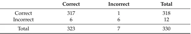
the same testing set, revealed it to be statistically significant at the 95% level of confidence (Table13). Specifically, given the seven discordant cases observed (Table13), Equation (4) yieldsz= 1.889.

The difference in accuracy between the classifications of the testing sets by the two selected neural networks (Tables11and12) was attributable mostly to seven cases of sugar beet being commissioned into the potato class when the validation set formed using a stratified sample was used. As a result of these errors the producer’s accuracy for the sugar beet class declined from 99.00% when the validation sample acquired with a random sample was used to 93.00% when the validation sample had been generated with a stratified sample. The user’s accuracy for the potato class also differed for the classifications of the testing set obtained when using the validation set defined with random and stratified sampling, the accuracies being 96.00% and 77.42%, respectively.

Given that the testing set had been generated using a simple random sample design the variation in the number of cases per-class reflected the relative abundance of the classes in the region to be mapped. Critically, the size of the sample of cases for the potato class was approximately one quarter of that for the sugar beet class. As hypothesized, the overall accuracy of the testing set decreased when the stratified rather than random sample was used in validation because cases of an abundant class (sugar beet) were commissioned by a relatively rare class (potato). Thus, even in a situation such as that encountered here, in which the classes are very highly separable, the sample design used in the formation of the validation dataset can have a statistically significant effect on the overall accuracy of the final land cover map, as reflected in the accuracy of the classifications of the testing set (Tables11and12).

Table 11.Confusion matrix for the testing set from the network selected using a validation set formed by random sampling.

Class S W B C P G Total User’s (%)

S 99 0 1 0 0 0 100 99.00

W 0 96 0 0 1 0 97 98.97

B 0 2 52 0 0 0 54 96.30

C 0 0 0 34 1 0 35 97.14

P 1 0 0 0 24 0 25 96.00

G 0 1 0 0 0 18 19 94.74

Total 100 99 53 34 26 18 330

Producer’s (%) 99.00 96.97 98.11 100 92.31 100

Table 12.Confusion matrix for the testing set from the network selected using a validation set formed by stratified sampling.

Class S W B C P G Total User’s (%)

S 93 0 1 0 0 0 94 98.94

W 0 97 0 0 1 0 98 98.98

B 0 2 52 0 0 0 54 96.30

C 0 0 0 34 1 0 35 97.14

P 7 0 0 0 24 0 31 77.42

G 0 0 0 0 0 18 18 100

Total 100 99 53 34 26 18 330

Producer’s (%) 93.00 97.98 98.11 100 92.31 100

Table 13.Cross-tabulation of labelling from classifiers using random (columns) and stratified (rows) validation sets for the remotely sensed data.

Correct Incorrect Total

Correct 317 1 318

Incorrect 6 6 12

Appl. Sci.2017,7, 888 12 of 15

Finally, it was also evident that the networks selected for the analyses of the remotely-sensed data differed, most notably in terms of architecture (Table10). When the validation set constructed with simple random sampling had been used, the data acquired in wavebands 1 and 8 were deemed unnecessary and, hence, only nine input units used. In addition this latter network also had fewer hidden units than the network selected when the validation set had been formed with a stratified sample. Overall, the network formed with the use of the validation sample acquired by random sampling was smaller and less complex than that selected when the validation set formed with a stratified sample was used. As such the network might be expected to be less likely to over-train and have a higher ability to generalize than that selected from the use of the validation sample formed via stratified sampling. Slightly different trends were observed for the simulated dataset. Here, however, it should be noted that a large number of networks of very different size, but very similar performance in terms of ability to classify the data, were generated, limiting the ability to comment on the issue; note, for example, that some candidate networks that yielded the same accuracy for the classification of the testing set after use of the random validation set had the smallest number of hidden units.

The results show that the design of the validation sample has a significant effect on classification by a neural network. Thus, the sample design used to form the validation set should be considered carefully when using neural networks. If, for example, there are constraints that limit design possibilities, it may be possible to make simple adaptations to standard practice. For example, if a stratified sample must be used for the validation sample, then this feature of the dataset should be accounted for in the assessment of the accuracy of the classification of the validation set. Thus, rather than use a standard confusion matrix, as indicated in Table5, the elements of the matrix could be converted from raw counts to proportions viapij =Wi

nij

ni· whereWiis the proportion of the area

mapped as classi[18]. The use of this approach, for example, shows that the estimated accuracy with which the validation set formed by stratified sampling of the simulated data was slightly less (98.12%) than the naïve assessment of the matrix (98.75%) and may indicate that the network it is associated with is, therefore, less attractive as a candidate for the task at hand than it first appears from the naïve assessment. Alternatively, if the focus of the application is on a subset of the classes it may be sensible to weight errors differentially or focus on only on the classes of interest rather than use overall accuracy. Critically, consideration needs to be given to the design of the validation sample in classification by a neural network. It should also be noted that this is only one small part of a set of broader validation issues that should be considered in the use of neural networks [47].

4. Conclusions

Acknowledgments:The ATM data were acquired through the European AgriSAR campaign and the research benefits from earlier work with colleagues, notably Manoj Arora, which is gratefully acknowledged. The neural network analyses were undertaken with the Trajan package. The map in Figure2was obtained from OpenStreetMap which are available under the Open Database Licence; further details athttp://www.openstreetmap.org/copyright.

Conflicts of Interest:The author declares no conflict of interest. The founding sponsors had no role in the design of the study; in the collection, analyses, or interpretation of data, in the writing of the manuscript, and in the decision to publish the results.

References

1. Tso, B.; Mather, P.M.Classification Methods for Remotely Sensed Data, 2nd ed.; Taylor & Francis: London, UK; New York, NY, USA, 2001.

2. Mas, J.F.; Flores, J.J. The application of artificial neural networks to the analysis of remotely sensed data.

Int. J. Remote Sens.2008,29, 617–663. [CrossRef]

3. Jensen, R.R.; Hardin, P.J.; Yu, G. Artificial neural networks and remote sensing. Geogr. Compass2009,3, 630–646. [CrossRef]

4. Yue, J.; Zhao, W.; Mao, S.; Liu, H. Spectral-spatial classification of hyperspectral images using deep convolutional neural networks.Remote Sens. Lett.2015,6, 468–477. [CrossRef]

5. Li, L.; Chen, Y.; Xu, T.; Huang, C.; Liu, R.; Shi, K. Integration of Bayesian regulation back-propagation neural network and particle swarm optimization for enhancing sub-pixel mapping of flood inundation in river basins.Remote Sens. Lett.2016,7, 631–640. [CrossRef]

6. Peddle, D.R.; Foody, G.M.; Zhang, A.; Franklin, S.E.; LeDrew, E.F. Multi-source image classification II: An empirical comparison of evidential reasoning and neural network approaches.Can. J. Remote Sens.1994,

20, 396–407. [CrossRef]

7. Lu, D.; Weng, Q. A survey of image classification methods and techniques for improving classification performance.

Int. J. Remote Sens.2007,28, 823–870. [CrossRef]

8. Serpico, S.B.; Bruzzone, L.; Roli, F. An experimental comparison of neural and statistical non-parametric algorithms for supervised classification of remote-sensing images.Pattern Recognit. Lett.1996,17, 1331–1341.

[CrossRef]

9. Paola, J.D.; Schowengerdt, R.A. A review and analysis of backpropagation neural networks for classification of remotely-sensed multi-spectral imagery.Int. J. Remote Sens.1995,16, 3033–3058. [CrossRef]

10. Kavzoglu, T.; Mather, P.M. The use of backpropagating artificial neural networks in land cover classification.

Int. J. Remote Sens.2003,24, 4907–4938. [CrossRef]

11. Pal, M.; Foody, G.M. Evaluation of SVM, RVM and SMLR for accurate image classification with limited ground data.IEEE J. Sel. Top. Appl. Earth Obs. Remote Sens.2012,5, 1344–1355. [CrossRef]

12. Foody, G.M.; Pal, M.; Rocchini, D.; Garzon-Lopez, C.X.; Bastin, L. The sensitivity of mapping methods to reference data quality: Training supervised image classifications with imperfect reference data.ISPRS Int. J.

Geo Inf.2016,5, 199. [CrossRef]

13. Antoniou, V.; Fonte, C.C.; See, L.; Estima, J.; Arsanjani, J.J.; Lupia, F.; Minghini, M.; Foody, G.; Fritz, S. Investigating the feasibility of geo-tagged photographs as sources of land cover input data.ISPRS Int. J.

Geo Inf.2016,5, 64. [CrossRef]

14. Kavzoglu, T. Increasing the accuracy of neural network classification using refined training data.

Environ. Model. Softw.2009,24, 850–858. [CrossRef]

15. Foody, G.M.; McCulloch, M.B.; Yates, W.B. The effect of training set size and composition on artificial neural network classification.Int. J. Remote Sens.1995,16, 1707–1723. [CrossRef]

16. Zhuang, X.; Engel, B.A.; Lozano-Garcia, D.F.; Fernandez, R.N.; Johannsen, C.J. Optimisation of training data required for neuro-classification.Int. J. Remote Sens.1994,15, 3271–3277. [CrossRef]

17. Foody, G.M. Hard and soft classifications by a neural network with a non-exhaustively defined set of classes.

Int. J. Remote Sens.2002,23, 3853–3864. [CrossRef]

18. Olofsson, P.; Foody, G.M.; Herold, M.; Stehman, S.V.; Woodcock, C.E.; Wulder, M.A. Good practices for estimating area and assessing accuracy of land change.Remote Sens. Environ.2014,148, 42–57. [CrossRef] 19. Stehman, S.V. Basic probability sampling designs for thematic map accuracy assessment.Int. J. Remote Sens.

Appl. Sci.2017,7, 888 14 of 15

20. Piper, J. Variability and bias in experimentally measured classifier error rates.Pattern Recognit. Lett.1992,13, 685–692. [CrossRef]

21. Garson, G.D.Neural Networks: An Introductory Guide for Social Scientists; Sage: London, UK, 1998.

22. Ahmad, S.; Tesauro, G. Scaling and generalisation in neural networks: A case study. InProceedings 1988

Connectionist Models Summer School; Touretzky, D., Hinton, G., Sejnowsjki, T., Eds.; Morgan Kaufmann:

San Mateo, CA, USA, 1989; pp. 3–10.

23. Foody, G.M. The significance of border training patterns in classification by a feedforward neural network using back propagation learning.Int. J. Remote Sens.1999,20, 3549–3562. [CrossRef]

24. Li, C.; Wang, J.; Wang, L.; Hu, L.; Gong, P. Comparison of classification algorithms and training sample sizes in urban land classification with Landsat thematic mapper imagery.Remote Sens.2014,6, 964–983. [CrossRef] 25. Silva, J.; Bacao, F.; Dieng, M.; Foody, G.M.; Caetano, M. Improving specific class mapping from remotely

sensed data by cost-sensitive learning.Int. J. Remote Sens.2017,38, 3294–3316. [CrossRef]

26. Ma, X.; Tong, X.; Liu, S.; Luo, X.; Xie, H.; Li, C. Optimized sample selection in SVM classification by combining with DMSP-OLS, Landsat NDVI and GlobeLand30 products for extracting urban built-up areas.

Remote Sens.2017,9, 236. [CrossRef]

27. Foody, G.M.; Mathur, A. Toward intelligent training of supervised image classifications: Directing training data acquisition for SVM classification.Remote Sens. Environ.2014,93, 107–117. [CrossRef]

28. Chang, E.I.; Lippmann, R.P. Using genetic algorithms to improve pattern classification performance.

InAdvances in Neural Information Processing Systems; Lippmann, R.P., Moody, J.E., Touretzky, D.S., Eds.;

Morgan Kaufmann: San Mateo, CA, USA, 1991; Volume 3, pp. 797–803.

29. Mathur, A.; Foody, G.M. Crop classification by support vector machine with intelligently selected training data for an operational application.Int. J. Remote Sens.2008,29, 2227–2240. [CrossRef]

30. Du, P.; Xia, J.; Zhang, W.; Tan, K.; Liu, Y.; Liu, S. Multiple classifier system for remote sensing image classification: A review.Sensors2012,12, 4764–4792. [CrossRef] [PubMed]

31. Foody, G.M.; Mathur, A. The use of small training sets containing mixed pixels for accurate hard image classification: Training on mixed spectral responses for classification by a SVM.Remote Sens. Environ.2006,

103, 179–189. [CrossRef]

32. Mueller, A.V.; Hemond, H.F. Statistical generation of training sets for measuring NO3−, NH4+and major ions in natural waters using an ion selective electrode array.Environ. Sci. Process. Impacts2016,18, 590–599.

[CrossRef] [PubMed]

33. Bishop, C.M.Neural Networks for Pattern Recognition; Oxford University Press: Oxford, UK, 1995.

34. Lek, S.; Giraudel, J.L.; Guegan, J.-F. Neuronal networks: Algorithms and architectures for ecologists and evolutionary ecologists. InArtificial Neuronal Networks. Application to Ecology and Evolution; Lek, S., Guegan, J.-F., Eds.; Springer: Berlin, Germany, 2000; pp. 3–27.

35. Fardanesh, M.T.; Ersoy, O.K. Classification accuracy improvement of neural network classifiers by using unlabeled data.IEEE Trans. Geosci. Remote Sens.1998,36, 1020–1025. [CrossRef]

36. Twomey, J.M.; Smith, A.E. Bias and variance of validation methods for function approximation neural networks under conditions of sparse data.IEEE Trans. Syst. Man Cybern. Part C1998,28, 417–430. [CrossRef] 37. Prechelt, L. Automatic early stopping using cross validation: Quantifying the criteria.Neural Netw.1998,11,

761–767. [CrossRef]

38. Setiono, R. Feedforward neural network construction using cross validation. Neural Comput. 2001, 13, 2865–2877. [CrossRef] [PubMed]

39. Huynh, T.Q.; Setiono, R. Effective neural network pruning using cross-validation. In Proceedings of the IEEE International Joint Conference on Neural Networks, Montreal, QC, Canada, 31 July–4 August 2005; Volume 2, pp. 972–977.

40. Lee, C.; Landgrebe, D.A. Decision boundary feature extraction for neural networks.IEEE Trans. Neural Netw.

1997,8, 75–83. [CrossRef] [PubMed]

41. Zhang, G.; Hu, M.Y.; Patuwo, B.E.; Indro, D.C. Artificial neural networks in bankruptcy prediction: General framework and cross-validation analysis.Eur. J. Oper. Res.1999,116, 16–32. [CrossRef]

42. Pal, M.; Mather, P.M. Support vector machines for classification in remote sensing.Int. J. Remote Sens.2005,

26, 1007–1011. [CrossRef]

44. Mas, J.F.; Puig, H.; Palacio, J.L.; Sosa-López, A. Modelling deforestation using GIS and artificial neural networks.Environ. Model. Softw.2004,19, 461–471. [CrossRef]

45. Foody, G.M. Thematic map comparison: Evaluating the statistical significance of differences in classification accuracy.Photogramm. Eng. Remote Sens.2004,70, 627–633. [CrossRef]

46. Agresti, A.Categorical Data Analysis, 2nd ed.; Wiley: New York, NY, USA, 2002.

47. Humphrey, G.B.; Maier, H.R.; Wu, W.; Mount, N.J.; Dandy, G.C.; Abrahart, R.J.; Dawson, C.W. Improved validation framework and R-package for artificial neural network models.Environ. Model. Softw.2017,92, 82–106. [CrossRef]