Effect of wettability on two-phase quasi-static
1
displacement: validation of two pore scale modeling
2
approaches
3
Rahul Vermaa, Matteo Icardib,c,d, Maˇsa Prodanovi´ca
4
aPetroleum and Geosystems Engineering, University of Texas at Austin, 200 E Dean 5
Keaton, Stop C0300, Austin, TX 78712-1585, USA 6
b
Mathematics Institute, Zeeman Building, University of Warwick, Coventry, CV4 7AL 7
cDivision of Computer, Electrical and Mathematical Sciences and Engineering, King 8
Abdullah University of Science and Technology, 23955-6900 Thuwal, Saudi Arabia 9
dInstitute of Computational Engineering and Sciences, University of Texas at Austin, 10
TX 78712-1585, USA 11
Abstract 12
1. Introduction 13
In this work, we focus on the displacement of two immiscible phases in
14
the subsurface, under variable wettability conditions, for example, in the
15
context of movement of oil and water in hydrocarbon reservoirs, or water
16
and non-aqueous phase liquids (NAPL) in soil. Wettability, as quantified by
17
the contact angles, influences oil and gas recovery processes like
waterflood-18
ing [1, 2] and other subsurface flow fields like carbon sequestration [3, 4],
19
pollutant migration and remediation processes in subsurface, transport of
20
dissolved minerals, colloids or contaminants, in dissolution and precipitation
21
processes, modeling of groundwater aquifers and so on [5].
22
Wettability is affected by rock mineralogy, organic deposits like bitumen,
23
and surface roughness of the rocks [1]. Given the complexity of capturing
24
this in a real rock, all modeling studies resort to simplifications. Field scale
25
simulators use averaged flow equations like Darcy’s law in combination with
26
mass conservation to model flow. In these simulators, wettability is
incorpo-27
rated into a J-function, which relates the capillary pressure and saturation
28
in a given porous medium [6, 7, 8]. The J-function is an empirical
relation-29
ship whose parameters are fit to experiments, and is therefore only indirectly
30
related to the actual contact angle at the pore scale. As such, it is difficult
31
to relate spatial and temporal wettability changes in the porous medium to
32
the final J-function for the representative elementary volume (REV). For a
33
more detailed study, one can focus on a much smaller system - modeling
34
flow in individual rock pores. These pore scale studies can be performed on
35
two or three dimensional images of small rock samples. Upon obtaining the
36
detailed pore structure of a rock via techniques such as X-ray
microtomog-37
raphy [9], there are multiple approaches for simulating flow (for a review see
38
Meakin and Tartakovsky [10]). There exist two broad categories of methods:
39
direct simulation on the pore image, or simplifying the image into a network
40
of simplified pores (openings) and throats (tight spots). The latter speeds
41
up simulations due to analytical solutions for flux through each throat [11],
42
allowing simulations over larger volumes than those used in direct
simula-43
tion. There is a lot of network modeling work for wettability problems [11],
44
but that is outside the scope of this work.
45
For direct simulations, the most popular methods are Navier-Stokes
46
based solvers [5]. Here, the full Navier-Stokes equations are solved in the
47
pore space with an additional equation for the interface and additional terms
48
to model surface tension forces. They are based on discretizing the flow
do-49
main into a computational grid. The finite-volume discretization can handle
50
very complex computational grids (e.g., with arbitrary shaped cells, and
cal or adaptive refinements), but building the grids can be considered a
52
delicate separate modeling step that requires accurate validation [12]. This,
53
together with their direct applicability on voxelized rock microstructure
im-54
ages, is the reason why simpler uniform Cartesian grids have gained
popu-55
larity. These are generally less accurate due to the poor representation of
56
the curved boundaries and the absence of local refinements. However they
57
can have important advantages in data storage and parallelization. The
lat-58
tice Boltzmann method, for example, is based on such a discretization [5].
59
One of the problems associated with the direct simulation of pore images
60
is the intrinsic difficulty in a robust validation, which is able to distinguish
61
between the several sources of errors and uncertainties associated with the
62
image pre-processing, sample size, geometry and equation discretization [13].
63
This is an important reason to further develop benchmark and validation
64
studies for geometries described analytically, like the one proposed in this
65
work. Despite these challenges, pore scale simulation enables improvements
66
of macroscopic models by taking into account different factors like topology
67
of the medium, heterogeneities, and changes in wettability.
68
In multiphase flow pore scale simulations, the interface represents a
mov-69
ing discontinuity in the domain and is difficult to handle numerically. In
70
this paper, we consider two techniques for modeling interface movement:
71
a variational formulation of the level set method [14], and the volume of
72
fluid method, implemented in theinterFoam solver, slightly modified
start-73
ing from the version released withinOpenFOAM 2.3.0. The level set method
74
was first proposed by Osher and Sethian in their seminal work [15]. The
75
method has since been applied for a wide variety of applications: from
image-76
processing and modeling flames to multiphase flows, and was introduced to
77
model quasi-equilibrium fluid/fluid interface movement in porous media by
78
Prodanovi´c and Bryant [16]. The method was used for simulating drainage
79
and imbibition in a porous medium of arbitrary geometry, when the
con-80
tact angle is zero. By defining the location and propagation of the interface
81
in an implicit manner, the level set method automatically handles
opera-82
tions such as interface splitting and merging. This is particularly useful for
83
tracking movement of an interface in a porous medium where phenomena
84
like snap-off and trapping often take place. Doing this using an explicitly
85
defined interface, such as by front tracking, would be generally more time
86
consuming, due to interface complexity in the pore space [17]. The level
87
set method has already been widely used for two-phase flow applications for
88
incompressible fluid flow [18]. Zhao et al. [19] proposed a variational
ap-89
proach for problems involving solid and fluid domains with different surface
90
and bulk energies. The level set method can also be extended for modeling
flow of more than two phases, for example by representing each interface
92
by its own level set function [20]. Level set methods suffer from mass loss,
93
especially in underresolved regions. Enrightet al. [21] addressed it using a
94
modification called the particle level set method. For further details about
95
the level set method we refer to the textbooks by Osher and Sethian on the
96
topic [22, 23].
97
The other technique we are using is a classical fluid dynamics solver
com-98
bined with a volume of fluid (VOF) method [24] for interface propagation.
99
At its core, VOF is similar to level set techniques. The original geometric
100
version of VOF uses explicit reconstruction of the interface in each cell (e.g.,
101
the so-called Piecewise-Linear Interface Calculation (PLIC) VOF), while the
102
algebraic version implemented in the open-source codeOpenFOAMis, in our
103
opinion, preferable when complex meshes with arbitrary shaped cells are
un-104
avoidable. This method has been recently used for pore-scale simulations
105
by many authors [25, 26, 27, 28, 29]. The main limitation of this
imple-106
mentation is the appearance of “parasitic” (or “spurious”) currents that can
107
significantly affect the accuracy near the interface. These unphysical
veloc-108
ity oscillations typically scale as the inverse of the capillary number (ratio
109
of viscous to capillary forces) and cannot be removed by refining the mesh.
110
They are caused by the continuous representation of surface tension forces,
111
across the discontinuity represented by the interface.
112
Some earlier works have focused on comparison of the level set method’s
113
accuracy with respect to the volume of fluid method in classical two-phase
114
flow benchmarks. For example, Sussman and Puckett (2000) [30] compared
115
the two methods, and proposed a coupled level set and volume of fluid
116
method. A later validation work was done by Gerlach et al. (2006) [31],
117
who studied an equilibrium rod, a capillary wave and the Rayleigh-Taylor
in-118
stability to compare three different volume of fluid formulations. Some other
119
authors have commented on the accuracy of the volume of fluid method for
120
capturing curvatures ([22]), which are independent of the capillary number
121
effects, but the volume of fluid method has also evolved since then, and
122
contemporary validation exercises have not been carried out. A more recent
123
validation effort was by Rabbani et al. [32], who calculated drainage
cur-124
vatures using the volume of fluid method in simple, constant cross section
125
geometries of the type used in pore network models. However, they did
126
not report on any parasitic currents which typically appear for low capillary
127
number flows.
128
The objective of this work is to perform a validation study in
capil-129
lary dominated slow displacement (where the interface can be considered
130
in equilibrium) under uniform wettability conditions in geometries where
either analytical solutions or reliable experimental data is available. We
132
consider the semi-analytical solutions in simple 3D geometries formed by
133
different sphere arrangements by Mason and Morrow [33]. These analytical
134
solutions, derived from further geometrical simplifications, were proven to
135
be very accurate for a wide range of contact angles and geometrical
parame-136
ters, through validation against experimental curvature measurements. We
137
note that when Jettestuenet al. first proposed the variational formulation
138
for contact angles, they did carry out a validation exercise. However, they
139
only did it for either 2D cases, or for 3D cases of constant cross-section. We
140
demonstrate that the formulation needs an additional modification in order
141
to get good results for 3D geometries of non-uniform cross-sections. This
142
simple, yet three-dimensional, set of pore geometries are ideal for validation
143
of numerical methods. A large amount of experimental work exists using
144
micromodels [34], X-ray computed microtomography [35, 9] and on the lab
145
scale [36, 37, 38]. X-ray tomography allows for direct imaging of fluid
distri-146
butions in more complex geometries, including finding local contact angles
147
([39, 40, 41]), in 3D. However, the experiments are non-trivial and flow field,
148
contact angles and correct curvatures in tighter pore spaces are still difficult
149
to map, which makes inter-comparison with simulation challenging. Our
150
work here is a step in that direction.
151
We present here results for two commonly used approaches, namely an
152
equilibrium level set formulation, and a full Navier-Stokes model with
al-153
gebraic VOF method. The latter, despite being designed for more
gen-154
eral dynamic calculations, is here modified to be able to compute efficiently
155
the steady state (equilibrium) through an over-damped pseudo-time
step-156
ping. This is, to the authors’ knowledge, the first attempt to validate these
157
two interface tracking methods with analytical results in an asymmetric,
158
converging-diverging geometry, typical in realistic porous media. The
re-159
sults can help assess the accuracy and usability of these methods for more
160
complex problems or random wettability patterns, and for upscaling
capil-161
lary pressure models in Darcy-scale equations. The critical curvatures for
162
drainage obtained by these models can also serve as input for drainage in
163
throats in pore network models.
164
There are some other works based on the lattice Boltzmann method,
165
which incorporate uniform and mixed wettability for predicting relative
per-166
meability in porous media [42, 43]. However, they do not make attempts
167
to validate small-scale multiphase displacements in a converging-diverging
168
porous media geometry. Validation is usually done using a drop on flat
169
surface, or a straight duct [44].
2. Methods 171
2.1. The level set method, with imposition of contact angle
172
The method introduced by Prodanovi`c and Bryant [16] models
displace-173
ment of immiscible fluids with zero contact angles in arbitrarily complex
174
geometries. It is based on the following level set evolution equation:
175
∂tφ+ (a−bκ)|∇φ|+V~ · ∇φ= 0 (1)
The level set function φ is defined at each grid point throughout the
176
domain of interest as the distance from the wetting/non-wetting fluid
in-177
terface, which is the zero level set. The level set functionφ is defined such
178
that it is positive “outside”, or on the side on convexity, and negative on
179
the concave side. For instance, in a two-phase porous media formulation,
180
φ >0 could denote the wetting phase, and φ < 0 denotes the non-wetting
181
phase and solid grain together (the choice of sign is, of course, arbitrary).
182
As the interface advances, the φ function is updated throughout the
do-183
main according to the level set equation. Defining the interface implicitly
184
means that changes in the topology of the fluid phases, such as snap-off and
185
merging of fluid menisci, are handled automatically.
186
Equation (1) governs the evolution of the function φin space while
im-187
posing interface speed. The term a is the speed of the interface normal to
188
itself - it can be viewed as a pressure-like term. The curvature-dependent
189
term bκ acts opposite to the imposed normal speed a. b determines how
190
strong the effect of curvature is - it is an interfacial tension-like term, and
191
is always positive for stability of the numerical method. V~ represents the
192
external advective field. The pore-grain boundary is defined by a separate
193
level set function ψ, such that the boundary is whereψ= 0.
194
Based on Equation (1), Jettestuen et al. [14] proposed a variational
195
approach to model contact angles in porous media. In their formulation,
196
in the main pore space, the sum a−bκ represents the difference between
197
imposed capillary pressure and the surface tension force (reproducing the
198
Young-Laplace equation), while near the boundaries,a,bandV~ are modified
199
to impose contact angles. We adopt their approach to get the following
200
modified level set equation:
201
φt+{H(−ψ)κ0−S(ψ)H(ψ)Ccosβ|∇ψ|}|∇φ|
+S(ψ)H(ψ)C∇ψ· ∇φ=H(−ψ)κφ|∇φ|
(2)
Here,H() denotes a Heaviside function, and is given by:
H(ψ) =
0, ψ <0
1 2+
ψ 2+
1 2πsin
πψ
, −≤ψ≤
1, ψ >
(3)
where is set to 1.5∆x, and ∆x is the numerical cell length. Terms
203
meant to take effect in the pore space are multiplied by H(−ψ), whereas
204
the solid phase terms are multiplied byH(ψ). θ=π−β is the contact angle
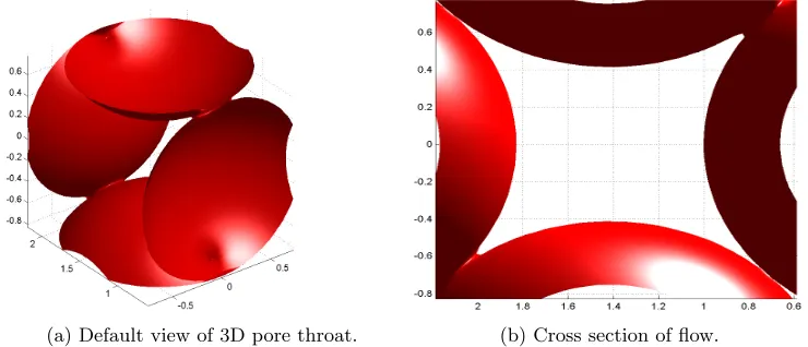
205
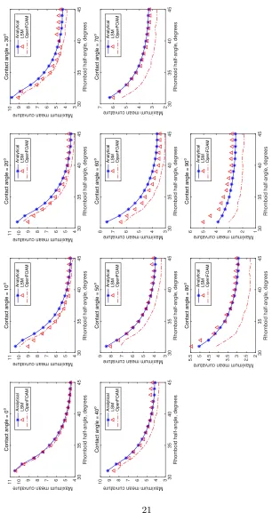
imposed on the medium (see Figure 1), whereβ is the angle enclosed by the
206
normals~nφand ~nψ. Thus, the modified level set equation works by impos-207
ing a velocity near the contact line such that the direction of the velocity
208
vector and the gradient vector of the mask form the desired contact angle.
209
Away from the boundary, we impose only the Young-Laplace equation. The
210
diffusive term associated with the zero level set curvature κφ in Equation 211
(2) smooths the level set function so that we get one single smooth interface
212
despite having different speeds of propagation of the interface near and far
213
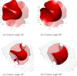
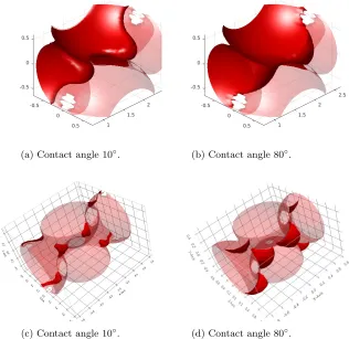
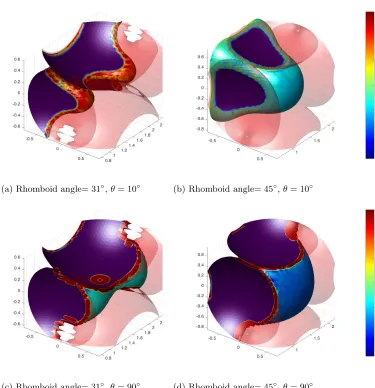
from the boundary. The curvatureκφis given by: 214
κφ=∇ ·
∇φ
|∇φ| (4)
κ0 is the imposed normal speed on the interface in the pore space. This 215
is slightly different from the quantityain the original level set equation, as
216
aincludes terms both in the pore space and near the boundary. S() is the
217
sign function which ensures that the contact angle propagates away from
218
the walls, and hence ensures numerical stability,
219
S(φ) = p φ
φ2+|∇φ|2(∆x)2 (5)
C is a constant that was used in Jettestuen et al. [14] to scale the
220
contact angle and curvature parts of the velocity. By trial and error, we
221
found it enough to set it equal to one. The level set equation must also be
222
periodically reinitialized to make sure that the gradients inφdo not become
223
too large. The default reinitialization equation was used, and is given by:
224
φt+S(φ)(|∇φ| −1) = 0 (6)
By imposing different values of the contact angle at different locations,
225
mixed wettability conditions can be simulated. A simple example is shown
226
in Jettestuenet al. [14], but we do not use it here.
227
Initially, we introduce a meniscus of low initial curvature into the
do-228
main, and advance it until it reaches an equilibrium position in the given
geometry. The speed at which the meniscus approaches the pore throat
230
must be low enough so that it does not simply exit the simulation volume
231
without reaching an equilibrium position. This is different from the
com-232
pressible model used by Prodanovi´c & Bryant [45], but it does not affect the
233
ultimate critical curvature.
[image:9.612.216.395.207.321.2]234
Figure 1: Imposition of contact angle using level set methods.
To simulate a drainage process, at every step, the curvature is increased
235
by ∆κ until the steady state solution is found. Therefore, the “time” t
236
defined in Equation (1) is a parameter without physical meaning.
237
Masking is enforced at every time step with some overlap, so that,
238
φ(x, t) + p ≤ ψ, where p is the overlap, measured in the grid spacing
239
∆x. This is a key difference in our methodology versus that introduced
240
in Jettestuen et al. [14]. They also have an overlap in the main equation,
241
but it is not enforced during the masking process. The overlap was found
242
necessary for accuracy as the contact angle became larger. When the
con-243
tact angle is closer to 0◦, no overlap was necessary. As the contact angle
244
increased (beyond 30◦), the overlap between the pore space and the grain
245
space was increased gradually, up to a maximum overlap of one grid cell.
246
For 40◦, the overlap was 0.3 grid cells, then for contact angle 50◦ it was
247
0.5, and finally the overlap was increased to one grid cell by contact angle
248
60◦, and held constant for greater angles. The method is stable without this
249
overlap, but it gave a much better match to analytical values. Having an
250
overlap is not physical. However, it allows for formation of contact angles
251
between different interfaces (the cusp is not a possible solution to a level set
252
equation that contains a diffusive curvature term) and does not affect the
253
equilibrium solution as long as overlap regions belonging to two portions of
254
grain boundary do not touch. It is thus intuitive that the size of the overlap
255
is related to the contact angle.
256
An imbibition simulation would proceed by taking the endpoint of a
drainage simulation as the starting point. Curvature is decreased step by
258
step, just as it was increased for the previous case. In this work, we have
259
not performed any imbibition simulations.
260
The equation was solved using the MATLAB level set toolbox written
261
by Ian Mitchell [46, 47]. The time derivative is approximated with a
third-262
order accurate total variation diminishing (TVD) Runge-Kutta integration
263
scheme. The Courant-Friedrichs-Lewy (CFL) conditions restrict the size of
264
the timestep. For the normal and convective terms, the gradients are
approx-265
imated by an upwind third order accurate essentially non-oscillatory (ENO)
266
finite difference scheme. The WENO (weighted essentially non-oscillatory)
267
scheme is more accurate, but it did not improve the quality of our results,
268
so we use the ENO scheme throughout. For the curvature velocity term, the
269
mean curvature κ is approximated using a centered second order accurate
270
finite difference approximation. This is also used in post-processing the
re-271
sults when we want to compute the distribution of curvature values on the
272
interface. Finally, as explained earlier, the level set equation is reinitialized
273
every few time steps using the reinitialization equation in order to maintain
274
|∇φ|= 1. Further details of individual numerical schemes can be found in
275
the book by Osher and Fedkiw [22].
276
2.2. Finite volume and volume-of-fluid methods
277
The volume of fluid method is a numerical technique used in the open
278
source software OpenFOAM to track interfaces in multiphase flows. In this
279
implementation the location and velocity of the fluid/fluid interface is
up-280
dated by using the Navier-Stokes equations, in a coupled manner. The
281
motion of a single incompressible fluid is governed by the Navier-Stokes
282
equation along with the mass conservation equation. For incompressible
283
fluids, the mass conservation equation is given by:
284
∇ ·(~uρ) = 0 (7)
The Navier-Stokes equation on the other hand describes conservation of
285
momentum:
286
∂ρ~u
∂t +∇ ·(ρ~u~u) =−∇p+∇ ·(2µ ~E) +f~b (8)
Here, ρ,~u and µ describe the density, velocity field and viscosity of the
287
fluid, respectively. E~ is the rate of strain tensor, while p is the pressure
288
field. f~b is the external body force term, which can include gravity. So, 289
in the case of two immiscible fluids, the Navier-Stokes equation along with
290
mass conservation are solved for each fluid separately.
At the interface between the fluids, we need to impose continuity of
292
velocity and tangential stresses and maintain jump in the normal stress
293
(equivalent to the capillary pressure). This can be done by considering the
294
velocity to be continuous across the interface, Γ:
295
~
uΓ−=~uΓ+ (9)
The stress field must satisfy:
296
[−p~I+ 2µ ~E]Γ·~n=σκ~n (10)
σ is the wetting/non-wetting fluid surface tension and~nis the normal to
297
the interface. The curvatureκ is twice the mean curvature of the interface
298
and is nominally the same as the one used in the level set method.
299
The above system of equations can be used to solve for the pressure and
300
velocity fields for each of the two fluids. The condition set on the velocity and
301
stress fields at the interface can be used to advect the interface. However, in
302
a numerical implementation this would lead to solving for moving boundary
303
conditions which is very complex and time-consuming, especially as we are
304
dealing with two separate fluid domains [26]. To get around this problem, the
305
VOF method was introduced by Hirt and Nichols in 1981 [24]. Essentially,
306
instead of solving two sets of Navier-Stokes equations and keeping track of
307
the fluid domain and shapes, we define an indicator function that identifies
308
which fluid is contained in a given fluid cell.
309
If one considers a domain having two phases, wetting (Pw) and
non-310
wetting (Pnw), then we can define an indicator function I(~x, t), 311
I(~x, t) =
1, ~x∈Pw
0, ~x∈Pnw
For cells which are completely wetting phase, the liquid fraction is 1,
312
while for non-wetting it is 0. The interface is located at I = 1/2, and is
313
indicated by the Dirac delta function around the interface,δΓ=δ(I−1/2). 314
We then get a modified form of the Navier-Stokes equation in the entire
315
domain:
316
∂ρ~u
∂t +∇ ·(ρ~u~u) =−∇ ·p+∇ ·(2µ ~E) + ~
fb+f~s (11)
where we can write for the density and viscosity fields:
317
ρ(~x, t) =ρwI(x, t~ ) +ρnw(1−I(~x, t))
µ(~x, t) =µwI(x, t~ ) +µnw(1−I(~x, t))
The additional term introduced,f~sdescribes the Laplace pressure acting 318
at the surface of discontinuity and is given by:
319
~
fs=σκ~nδΓ (13)
For numerical implementation, the term f~s is replaced by a continuum 320
surface force (CSF):
321
~
fv =σκ∇I (14)
~
fv tends tof~s as the thickness of the interface region tends to zero. The 322
curvature κ is calculated from the indicator function. It can be seen this
323
is the same as the curvature in the level set method, where the indicator
324
function replaces φ in Equation (4). Using mass conservation in
combina-325
tion with the modified Navier-Stokes equation (11), we finally get a simple
326
advection equation for the indicator function:
327
∂I
∂t +∇ ·(I~u) = 0 (15)
To counterbalance numerical diffusion, a non-linear convective term is
328
added to the equation, which acts as a shock that balances numerical
diffu-329
sion.
330
∂I
∂t +∇ ·(I~u) +∇ ·(I(1−I)u~r) = 0 (16)
where~uris a compression velocity. Its choice does not affect the solution 331
outside the interfacial region. Note that the indicator function defines the
332
interface implicitly as the 1/2 level set of I, and the advection equation for
333
the indicator function is related to the level set equation (Equation (1)). An
334
example smoothed indicator function is the Heaviside function, defined in
335
Equation (3).
336
At the solid boundaries, the fluids are constrained in the pore space by
337
requiring that the velocity component normal to the solid wall is zero. At
338
the triple-contact line, Young’s law determines the contact angle:
339
cosθ= σnw,s−σw,s
σ (17)
whereσnw,sis the non-wetting fluid/solid interfacial tension,σw,s is the 340
wetting fluid/solid interfacial tension.
341
For imposing the contact angle in our simulation, this is equivalent to
342
imposing the boundary condition:
343
~
where~ts is the unit tangential vector pointing into the wetting phase. 344
OpenFOAM uses finite volume discretization for the above equations for
345
mass and momentum conservation, and advection of the indicator function.
346
The advection equation (Equation (16)) is used to update the indicator
347
function values throughout the domain. This is then used to update fluid
348
properties throughout the domain, and calculate the surface force. Finally,
349
the coupling between the pressure and velocity equation (Equation (11)) is
350
performed by using the Pressure Implicit with Splitting of Operators (PISO)
351
implicit pressure correction procedure. Further details on the
implementa-352
tion of interFoam and the numerical schemes used may be looked up in
353
Deshpandeet al. [48].
354
In order to calculate critical curvatures, we employ a quasi-static
ap-355
proach similar to the level set method presented earlier. We increase the
356
pressure gradient in small steps, and allow the interface to reach
equilib-357
rium at each step. Since we are interested in only the equilibrium position,
358
and the equilibrium arises from the balance of the pressure gradient and
359
surface tension forces, we can arbitrarily choose the physical parameters
360
of the system (chosen dimensionless and unitary here). For the same
rea-361
son, we are allowed to arbitrarily add to the momentum equation extra
362
damping (Darcy-like) terms. In fact, despite significantly changing the
dy-363
namics of the interface, this does not change the equilibrium position (being
364
the additional term proportional to the velocity and, therefore vanishing
365
at equilibrium). The advantage of this approach is that we can arbitrarily
366
choose the Reynolds and capillary number to approach fast and smoothly
367
the equilibrium position, while controlling the parasitic currents. Further
368
details are shown in Appendix C. In addition, we use a special version of
369
the interFoam solver, with local time stepping (LTSInterFoam), to march in
370
pseudo-time with a pre-defined time step. This technique can maximize the
371
time step (therefore reducing the relaxation time) in each cell. The
result-372
ing iterations are therefore not physical and not related to evolution in real
373
time but simply represent internal iterations to reach the steady state. At
374
each equilibrium step, thanks to the equilibrium of forces guaranteed by the
375
Navier-Stokes equations, we get the equivalent curvature in the pore using
376
the Young-Laplace equation, with the stationary Navier-Stokes solution for
377
pressure at the two flow boundaries giving the capillary pressure, and the
378
surface tension value imposed by us. All these choices make the VOF solver
379
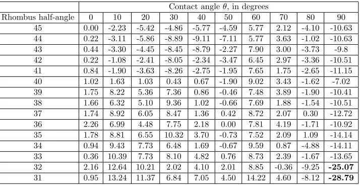
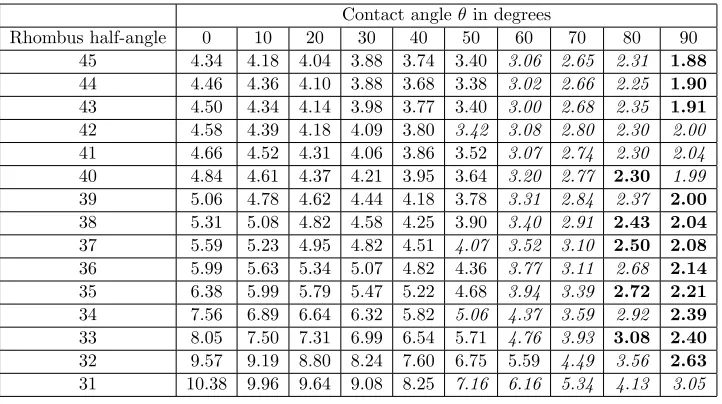
under study equivalent to the quasi-static level set formulation. The
remain-380
ing differences lie in the different equations solved, in the implementation of
381
curvature and the boundary conditions.
382
Since the finite-volume discretization is applicable both to structured
and unstructured grids1, we tested the solver on two types of grids: a
regu-384
lar Cartesian grid (the same one used for the level set method) and a grid
385
locally adapted to the interface. In both cases the mesh generator
snappy-386
HexMesh has been used to automatically generate the mesh from analytical
387
information on the sphere geometry. Preliminary results show no significant
388
differences for the mean curvature measured. This is due to the fact that no
389
explicit geometrical information about the interface is used by the solver.
390
The curvature and surface tension discretization is totally done based on the
391
concentration field. Therefore the shape of the cell close to the interface is
392
not very important when there is no flow occurring. For this reason in the
393
following results, only the simulations with the regular Cartesian grids are
394
presented.
395
2.3. Analytical and experimental observations
396
Mason and Morrow [33] published a semi-analytical calculation of the
397
maximum curvatures (also called critical curvatures) for the rhomboidal pore
398
for a range of contact angles and rhomboid pore angles, and experimentally
399
validated their results. In this work we compare our simulation results
400
against their semi-analytical values.
401
We briefly provide their methodology followed by them in Appendix B.
402
Further details may be obtained in their original work. For completeness,
403
we also provide their calculations in Appendix A.
404
1
(a) Default view of 3D pore throat. (b) Cross section of flow.
Figure 2: 3D pore throat geometry for rhomboid angle 45◦.
3. Results and Discussion 405
The results from the quasi-static level set and the Navier-Stokes
volume-406
of-fluid (OpenFOAM) solvers are compared with those obtained by Mason
407
and Morrow [33] for the actual pore throat geometries, like the one in Fig. 2.
408
The semi-analytical results are summarized in Table A.1. Values obtained
409
from both codes are also listed in the Appendix, in Tables A.2 and A.4.
410
The maximum mean curvature computation results for each contact angle
411
are shown in Figure 5. Errors for each case are reported in Tables A.3 and
412
A.5. The values and errors for running the level set method without the
413
overlap are presented in Tables A.6 and A.7, respectively.
414
Prior to performing simulations on 3D pore geometries for the level set
415
formulation, the technique was first tested on 2D geometries. The results
416
for those are available in [49]. The simulation results presented here follow
417
the analytical cases for which Mason and Morrow [33] determined maximum
418
mean curvatures. The rhomboid half-angles vary from 31◦ to 45◦.
Repre-419
sentative geometry is shown for rhomboid half-angle of 45◦ in Figure 2. For
420
each rhomboid half-angle, contact angle varied from 0◦ to 90◦. Errors for
421
each case are reported in Table A.3.
422
In the following figures, the solid walls are shown in transparent color
423
while the fluid interface is shown in red. The reconstruction of the interface
424
at equilibrium, with both codes, for rhomboid angles 45◦ and 31◦ and
con-425
tact angles 10◦ and 80◦ is reported in Figures 3 and 4. The dimensions of
426
the domain and the size of the mesh spacing are the same; however, since
427
data are stored in a different format, the figures may look slightly different
due to different visualization algorithm. These cases represent extremities in
429
contact angle as well as rhomboid half-angle and are hence good for
show-430
casing the method’s accuracy. MS-P theory predicts a divided meniscus
431
for rhomboid half-angle 31◦. As can be seen in Figure 4, this is effectively
432
captured in the simulations.
433
For performing the simulations with zero contact angle in the level set
434
method, we follow the recommendations of Jettestuenet al. [14] and use the
435
original LSMPQS software [50]. That code is in C/FORTRAN, and is also
436
otherwise faster than the modified method due to its simplicity. We obtain
437
an excellent match with the analytical solution. The OpenFOAM results
438
are also very good for this case. The grid spacing used here is 0.02. Note
439
that the disk/sphere radii in all examples is 1, and the reported grid spacing
440
and all lengths are relative to the radii. For the other cases (with contact
441
angle larger than zero) with the level set method, we used a slightly different
442
(MATLAB-based) implementation, and due to higher computational costs,
443
the grid spacing was set to 0.04. For consistency, the OpenFOAM results
444
shown in Figure 5 were also run with the same grid size of 0.04. A grid
445
convergence study was also performed for OpenFOAM, by making the grid
446
twice as fine (grid size 0.02). The results did not show significant
improve-447
ment. We present those results in the Appendix C. The results shown in
448
Figure 5 show both methods performing well for lower contact angles, while
449
the OpenFOAM solver has higher errors for high contact angles. In some
450
cases, the level set method seems to overshoot the analytical predictions for
451
high rhomboid angles. This is likely an artifact of the numerical overlap
452
imposed. As described in the previous section, the overlap between the pore
453
space and rock was used to ensure proper formation of the contact angle in
454
the level set method. The overlap is going to present problems when
simu-455
lating larger samples with narrow solid regions as discussed in Jettestuenet
456
al. [14]. The adaptive meshing schemes that will address the problem will
457
be investigated in future work. The OpenFOAM boundary conditions did
458
not require an overlap.
459
Another important aspect is the initial condition. A starting curvature
460
that allows the interface to find a stable position within the pore space in
461
general geometries is not known a priori which prompted the development
462
of the compressible model in [16]. In this work with simple pore throats, we
463
did not find it necessary to run the compressible model. It was enough to
464
guess a sensible starting value of the normal velocity term for all cases. We
465
choose a starting value of 0.15 for the normal velocity term κ0 and allow
466
the interface to find the equilibrium position (steady state solution to
Equa-467
tion (2)). For the OpenFOAM simulations, the relaxation to equilibrium is
(a) Contact angle 10◦. (b) Contact angle 80◦.
[image:17.612.142.456.219.529.2](c) Contact angle 10◦. (d) Contact angle 80◦.
(a) Contact angle 10◦. (b) Contact angle 80◦.
[image:18.612.164.480.226.533.2](c) Contact angle 10◦. (d) Contact angle 80◦.
solely driven by the imposed pressure drops at the boundaries and, for these
469
particular converging-diverging pores, every initial interface position gives
470
the same final equilibrium result. However, to speed up the computations,
471
the interface has always been placed in the middle of the domain and the
472
initial pressure drop set to a fraction (typically 0.8) of the reference
analyti-473
cal results. As already mentioned in the previous section, the pressure drop
474
is then increased until the interface reaches its maximum curvature
posi-475
tion before being transported out of the domain when the imposed pressure
476
becomes larger than the pore entry capillary pressure. We demonstrate
im-477
provements in convergence to equilibrium due to the damping term for two
478
extreme cases in figures C.12 and C.13 in Appendix C. The figures
com-479
pare changes in saturation and velocity at each capillary pressure step, with
480
and without the damping term. At each capillary pressure step, there is
481
a sharp jump in both velocities and saturations. As the system moves to
482
equilibrium, this dies out. Without the damping term, the jumps are more
483
extreme. This clearly shows the advantage of using the damping term, as
484
we achieve the same equlibrium condition faster.
485
A pertinent point on the actual calculation of the curvatures is that for
486
the level set method, we use the formulation proposed by Osher and Sethian
487
[22] in their original work (see Equation (4)). The level set code incorporates
488
that by calculating the curvatures at every grid point up to second order
489
accuracy. The difficulty here is that the actual interface passes in between
490
grid points, causing significant differences in accuracy of the method if one
491
chooses to take the nearest grid point for calculating curvatures instead of
492
the actual interface. Hence, we first found the exact interface coordinates,
493
and then interpolated the curvatures given at the grid points to find the
494
curvatures on all the points of the interface. The curvatures reported in
495
Table A.2 are the mean values of the curvatures from all the points on the
496
interface. Taking the mean value for the curvature is problematic in some of
497
the simulation cases as there is a wide spread in curvature values at different
498
points of the interface.
499
We exemplify this for contact angles 10◦ and 90◦, and rhomboid
half-500
angles 31◦ and 45◦ in Figure 6. For the first case (rhomboid angle 31◦),
501
we can see that the spread in values is quite high due to tight pore spaces
502
where solid surfaces are too close together and resolution should be finer.
503
This results in a high error when we compare the calculated mean curvature
504
with analytical values. Additionally, for the worst case of contact angle
505
90◦, the change in curvature values near the boundaries is much sharper,
506
but the diffusive nature of the level set method ensures a smooth interface.
507
For the second case (rhomboid angle 45◦), we can see that the interface is
much better resolved, and we get a lower final error, though in this case
509
also, a contact angle of 90◦ results in sharp changes in curvature near the
510
boundaries. The case for contact angle 90◦ has the highest errors, up to
511
25%. This case is like a piston moving across the pore, and this causes large
512
intersection regions between solid and non-wetting fluid phase. However,
513
even in this extreme contact angle, most of the cases have errors in the
514
range of 10%. This also highlights the importance of adaptive meshing
515
for imposition of contact angles. Near the solid-liquid-liquid contact line
516
at the boundary, we can have a much finer grid, with coarser grid cells
517
in the main pore space. So we can better capture the contact angle at
518
the boundary, with lesser computational expense. The curvatures are more
519
difficult to resolve in the same areas. Note that, for the level set method,
520
we already tried higher order accurate numerical schemes without much
521
improvement. For OpenFOAM, higher order accurate schemes for general
522
unstructured meshes are not available. Finer grid cells near the boundary
523
however can be added. Thus, adaptive meshing seems a logical course to
524
follow for future work on these methods. This will surely have a beneficial
525
effect in the local computations of curvatures. Whether this has an effect
526
on more general displacement problems is something that requires more
527
studies. The OpenFOAM results, in fact, suggest that a grid refinement
528
is not improving the overall capillary pressure estimated by the balance of
529
forces solved in the momentum equation. This mean that other factors (e.g.
530
the way the contact angle is imposed) might be important.
531
The overall results show promise for more general applications. Imaging
532
has the potential of informing us of the distribution of wettability on a
533
given rock sample by identification of the mineralogy and possible bitumen
534
coatings [51]. In that case, we could map surfaces of different wettability
535
and a method which can predict the behavior of capillary-dominated flow in
536
a given rock sample can be applicable. Jettestuenet al. [14] have shown the
537
method applied to simple mixed wet systems. However, it is likely that more
538
general porous media geometries would be more problematic. If one were to
539
attempt simulating flow in an image from a rock sample, the error margins
540
would likely be larger and a relatively small error (like the ones observed
541
here) might propagate to the macro-scale in a unpredictable way. Our future
542
work will also benchmark with other methods (such as the lattice Boltzmann
543
method) to increase awareness of potential limitations and to provide better
544
accuracy assessment of the methods.
30
35
40
45
Rhomboid half-angle, degrees
4 5 6 7 8 9 10
11 Maximum mean curvature
Contact angle = 0
o Analytical LSM OpenFOAM
30
35
40
45
Rhomboid half-angle, degrees
4 5 6 7 8 9 10
11 Maximum mean curvature
Contact angle = 10
o Analytical LSM OpenFOAM
30
35
40
45
Rhomboid half-angle, degrees
4 5 6 7 8 9 10
11 Maximum mean curvature
Contact angle = 20
o Analytical LSM OpenFOAM
30
35
40
45
Rhomboid half-angle, degrees
3 4 5 6 7 8 9
10 Maximum mean curvature
Contact angle = 30
o Analytical LSM OpenFOAM
30
35
40
45
Rhomboid half-angle, degrees
3 4 5 6 7 8 9
10 Maximum mean curvature
Contact angle = 40
o
Analytical LSM OpenFOAM
30
35
40
45
Rhomboid half-angle, degrees
3 4 5 6 7 8
9 Maximum mean curvature
Contact angle = 50
o Analytical LSM OpenFOAM
30
35
40
45
Rhomboid half-angle, degrees
3
4
5
6
7
8 Maximum mean curvature
Contact angle = 60
o Analytical LSM OpenFOAM
30
35
40
45
Rhomboid half-angle, degrees
2 3 4 5 6 7
Maximum mean curvature
Contact angle = 70
o Analytical LSM OpenFOAM
30
35
40
45
Rhomboid half-angle, degrees
2 2.5 3 3.5 4 4.5 5 5.5
Maximum mean curvature
Contact angle = 80
o Analytical LSM OpenFOAM
30
35
40
45
Rhomboid half-angle, degrees
1
2
3
4
5
6 Maximum mean curvature
Contact angle = 90
o Analytical LSM OpenFOAM
[image:21.612.140.446.122.699.2](a) Rhomboid angle= 31◦,θ= 10◦ (b) Rhomboid angle= 45◦,θ= 10◦
[image:22.612.148.523.188.576.2](c) Rhomboid angle= 31◦,θ= 90◦ (d) Rhomboid angle= 45◦,θ= 90◦
4. Conclusion 546
We have quantified the accuracy of two popular methods for capillarity
547
dominated quasi-static displacements in a set of converging-diverging pore
548
throat geometries, namely a level set method and an algebraic volume of fluid
549
(within the OpenFOAM software). Both methods perform well for lower
550
contact angles, though we observed better accuracy for the level set method
551
for contact angles more than 70◦, while both methods struggle with 90◦
552
contact angle. For other problems where viscosity (or gravity) plays a more
553
dominant role certainly Navier-Stokes based solvers such as OpenFOAM
554
are more appropriate, and this version of the level set method should not
555
be used.
556
Validation of numerical methods is most commonly done in constant
557
cross-section geometries since that is where analytical solutions exist.
Sim-558
ilar is true for widely accepted lattice Boltzmann methods. There is a gap
559
between testing in tubes [32] and simulation in larger geometries [43]. The
560
only way to test larger geometries is against experiments, which are not
561
always available.
562
This kind of validation is particularly important in larger geometries,
563
where it if often required to sacrifice some accuracy for much lower
com-564
putational time. One also may choose to use a lower precision numerical
565
scheme (like first order accuracy in time) to get results faster. The
pre-566
sented implementation of the level set method has not been optimized for
567
running large cases. In future work, an optimized code will be used to study
568
larger geometries as well as real rock images, where convergence criteria
569
could be relaxed a little for much lower computational time. Determining
570
when the simulation has converged is usually the judgment of the individual
571
user. Hence, as direct pore scale modeling approaches become more
popu-572
lar, validation against other codes and experimental results will be crucial
573
to check the overall reliability of the results.
574
We expect that these kind of validation studies will also become
in-575
creasingly important in other problems such as imbibition in porous media,
576
where most larger-scale models fail. Imbibition is more difficult to model
577
with quasi-static approaches than drainage. In the future we will
quan-578
tify the differences between quasi-static and dynamic approaches in
imbi-579
bition: while most of imbibition studies have been done using quasi-static
580
approaches due to computational complexity, it remains an open question if
581
they are adequate in describing ultimate fluid configuration (and also
rela-582
tive permeability).
5. Acknowledgements 584
This work was supported by the Gas EOR consortium at UT Austin
585
(RV), by NSF CAREER grant 1255622 (MP) and by the King Abdullah
586
University of Science and Technology (KAUST) (MI). MI was supported by
587
the Academic Excellency Alliance (AEA) UT Austin-KAUST project
“Un-588
certainty quantification for predictive modeling of the dissolution of porous
589
and fractured media” and by the KAUST SRI Center for Uncertainty
Quan-590
tification in Computational Science and Engineering.
6. References 592
[1] N. Morrow, Wettability and its effect on oil recovery, Journal of
593
Petroleum Technology 42 (12). doi:10.2118/21621-PA.
594
[2] N. Morrow, H. Lim, J. Ward, Effect of crude-oil-induced
wetta-595
bility changes on oil recovery, SPE Formation Evaluation 1 (1).
596
doi:10.2118/13215-PA.
597
[3] C. H. Pentland, R. El-Maghraby, S. Iglauer, M. J. Blunt, Measurements
598
of the capillary trapping of super-critical carbon dioxide in berea
sand-599
stone, Geophysical Research Letters 38 (6).
600
[4] S. Iglauer, A. Paluszny, C. H. Pentland, M. J. Blunt, Residual CO2
601
imaged with X-ray micro-tomography, Geophysical Research Letters
602
38 (21).
603
[5] M. J. Blunt, B. Bijeljic, H. Dong, O. Gharbi, S. Iglauer,
604
P. Mostaghimi, A. Paluszny, C. Pentland, Pore-scale imaging
605
and modelling, Advances in Water Resources 51 (2013) 197–216.
606
doi:10.1016/j.advwatres.2012.03.003.
607
[6] Y.-S. Wu, B. Bai, et al., Efficient simulation for low salinity
waterflood-608
ing in porous and fractured reservoirs, in: SPE Reservoir Simulation
609
Symposium, Society of Petroleum Engineers, 2009.
610
[7] M. Cil, J. C. Reis, M. A. Miller, D. Misra, et al., An examination of
611
countercurrent capillary imbibition recovery from single matrix blocks
612
and recovery predictions by analytical matrix/fracture transfer
func-613
tions, in: SPE Annual Technical Conference and Exhibition, Society of
614
Petroleum Engineers, 1998.
615
[8] A. Gupta, F. Civan, et al., An improved model for laboratory
measure-616
ment of matrix to fracture transfer function parameters in immiscible
617
displacement, in: SPE Annual Technical Conference and Exhibition,
618
Society of Petroleum Engineers, 1994.
619
[9] D. Wildenschild, A. P. Sheppard, X-ray imaging and analysis techniques
620
for quantifying pore-scale structure and processes in subsurface porous
621
medium systems, Advances in Water Resources 51 (2013) 217–246.
622
[10] P. Meakin, A. M. Tartakovsky, Modeling and simulation of
pore-623
scale multiphase fluid flow and reactive transport in fractured
and porous media, Reviews of Geophysics 47 (3) (2009) n/a–n/a.
625
doi:10.1029/2008RG000263.
626
[11] M. J. Blunt, M. D. Jackson, M. Piri, P. H. Valvatne, Detailed physics,
627
predictive capabilities and macroscopic consequences for pore-network
628
models of multiphase flow, Advances in Water Resources 25 (8–12)
629
(2002) 1069–1089. doi:10.1016/S0309-1708(02)00049-0.
630
[12] T. J. Baker, Mesh generation: Art or science?, Progress in Aerospace
631
Sciences 41 (1) (2005) 29–63.
632
[13] M. Icardi, G. Boccardo, R. Tempone, On the predictivity of pore-scale
633
simulations: Estimating uncertainties with multilevel monte carlo,
Ad-634
vances in Water Resources 95 (2016) 46–60.
635
[14] E. Jettestuen, J. O. Helland, M. Prodanovi´c, A level set method for
636
simulating capillary-controlled displacements at the pore scale with
637
nonzero contact angles, Water Resources Research 49 (8) (2013) 4645–
638
4661. doi:10.1002/wrcr.20334.
639
[15] S. Osher, J. A. Sethian, Fronts propagating with curvature-dependent
640
speed: Algorithms based on Hamilton-Jacobi formulations, Journal
641
of Computational Physics 79 (1) (1988) 12–49.
doi:10.1016/0021-642
9991(88)90002-2.
643
[16] M. Prodanovi´c, S. L. Bryant, A level set method for determining critical
644
curvatures for drainage and imbibition, Journal of Colloid and Interface
645
Science 304 (2) (2006) 442–458. doi:10.1016/j.jcis.2006.08.048.
646
[17] S. O. Unverdi, G. Tryggvason, A front-tracking method for viscous,
647
incompressible, multi-fluid flows, Journal of computational physics
648
100 (1) (1992) 25–37.
649
[18] E. Olsson, G. Kreiss, A conservative level set method for two phase
650
flow, Journal of Computational Physics 210 (1) (2005) 225–246.
651
doi:10.1016/j.jcp.2005.04.007.
652
[19] H.-K. Zhao, B. Merriman, S. Osher, L. Wang, Capturing the
be-653
havior of bubbles and drops using the variational level set
ap-654
proach, Journal of Computational Physics 143 (2) (1998) 495–518.
655
doi:10.1006/jcph.1997.5810.
[20] S. Esodoglu, P. Smereka, A variational formulation for a level set
repre-657
sentation of multiphase flow and area preserving curvature flow,
Com-658
munications in Mathematical Sciences 6 (1) (2008) 125–148,
mathemat-659
ical Reviews number (MathSciNet): MR2398000; Zentralblatt MATH
660
identifier: 1137.76067.
661
[21] D. Enright, R. Fedkiw, J. Ferziger, I. Mitchell, A hybrid particle level
662
set method for improved interface capturing, Journal of Computational
663
physics 183 (1) (2002) 83–116.
664
[22] S. Osher, R. Fedkiw, Level Set Methods and Dynamic Implicit Surfaces,
665
Springer, 2003.
666
[23] J. A. Sethian, Level Set Methods and Fast Marching Methods:
Evolv-667
ing Interfaces in Computational Geometry, Fluid Mechanics, Computer
668
Vision, and Materials Science, Cambridge University Press, 1999.
669
[24] C. W. Hirt, B. D. Nichols, Volume of fluid (vof) method for the
dynam-670
ics of free boundaries, Journal of computational physics 39 (1) (1981)
671
201–225.
672
[25] A. Ferrari, I. Lunati, Direct numerical simulations of interface dynamics
673
to link capillary pressure and total surface energy, Advances in Water
674
Resources 57 (2013) 19–31.
675
[26] A. Ferrari, I. Lunati, Inertial effects during irreversible meniscus
re-676
configuration in angular pores, Advances in Water Resources 74 (2014)
677
1–13.
678
[27] D. A. Hoang, V. van Steijn, L. M. Portela, M. T. Kreutzer, C. R.
679
Kleijn, Benchmark numerical simulations of segmented two-phase flows
680
in microchannels using the volume of fluid method, Computers & Fluids
681
86 (2013) 28–36.
682
[28] P. Horgue, F. Augier, P. Duru, M. Prat, M. Quintard, Experimental
683
and numerical study of two-phase flows in arrays of cylinders, Chemical
684
Engineering Science 102 (2013) 335–345.
685
[29] A. Q. Raeini, M. J. Blunt, B. Bijeljic, Modelling two-phase flow in
686
porous media at the pore scale using the volume-of-fluid method,
Jour-687
nal of Computational Physics 231 (17) (2012) 5653–5668.
[30] M. Sussman, P. Smereka, S. Osher, A level set approach for computing
689
solutions to incompressible two-phase flow, Journal of Computational
690
Physics 114 (1) (1994) 146–159. doi:10.1006/jcph.1994.1155.
691
[31] D. Gerlach, G. Tomar, G. Biswas, F. Durst, Comparison of
volume-692
of-fluid methods for surface tension-dominant two-phase flows,
693
International Journal of Heat and Mass Transfer 49 (34) (2006)
694
740–754. doi:10.1016/j.ijheatmasstransfer.2005.07.045.
695
URLhttp://www.sciencedirect.com/science/article/pii/S0017931005005314
696
[32] H. S. Rabbani, V. Joekar-Niasar, N. Shokri, Effects of intermediate
697
wettability on entry capillary pressure in angular pores, Journal of
698
Colloid and Interface Science 473. doi:10.1016/j.jcis.2016.03.053.
699
URLhttp://www.sciencedirect.com/science/article/pii/S0021979716301953
700
[33] G. Mason, N. R. Morrow, Effect of contact angle on
capil-701
lary displacement curvatures in pore throats formed by spheres,
702
Journal of Colloid and Interface Science 168 (1) (1994) 130–141.
703
doi:10.1006/jcis.1994.1402.
704
[34] M. A. Celia, P. C. Reeves, L. A. Ferrand, Recent advances in pore scale
705
models for multiphase flow in porous media, Reviews of Geophysics
706
33 (S2) (1995) 1049–1057. doi:10.1029/95RG00248.
707
[35] D. Wildenschild, C. Vaz, M. Rivers, D. Rikard, B. Christensen, Using
708
X-ray computed tomography in hydrology: systems, resolutions, and
709
limitations, Journal of Hydrology 267 (3) (2002) 285–297.
710
[36] G. M. Homsy, Viscous fingering in porous media, Annual Review of
711
Fluid Mechanics 19 (1) (1987) 271–311.
712
[37] D. B. Ingham, I. Pop, Transport phenomena in porous media III, Vol. 3,
713
Elsevier, 2005.
714
[38] M. T. Van Genuchten, P. Wierenga, Mass transfer studies in sorbing
715
porous media I. analytical solutions, Soil Science Society of America
716
Journal 40 (4) (1976) 473–480.
717
[39] M. Khishvand, A. Alizadeh, M. Piri, In-situ characterization of
wetta-718
bility and pore-scale displacements during two-and three-phase flow in
719
natural porous media, Advances in Water Resources 97 (2016) 279–298.
[40] M. Andrew, B. Bijeljic, M. J. Blunt, Pore-scale contact angle
measure-721
ments at reservoir conditions using x-ray microtomography, Advances
722
in Water Resources 68 (2014) 24–31.
723
[41] M. Andrew, H. Menke, M. J. Blunt, B. Bijeljic, The imaging of dynamic
724
multiphase fluid flow using synchrotron-based x-ray microtomography
725
at reservoir conditions, Transport in Porous Media 110 (1) (2015) 1–24.
726
[42] C. J. Landry, Z. T. Karpyn, O. Ayala, Pore-Scale Lattice Boltzmann
727
Modeling and 4d X-ray Computed Microtomography Imaging of
728
Fracture-Matrix Fluid Transfer, Transport in Porous Media 103 (3)
729
(2014) 449–468. doi:10.1007/s11242-014-0311-x.
730
URLhttps://link.springer.com/article/10.1007/s11242-014-0311-x
731
[43] C. J. Landry, Z. T. Karpyn, O. Ayala, Relative permeability of
732
homogenous-wet and mixed-wet porous media as determined by
733
pore-scale lattice Boltzmann modeling, Water Resources Research
734
50 (5) (2014) 3672–3689. doi:10.1002/2013WR015148.
735
URLhttp://onlinelibrary.wiley.com/doi/10.1002/2013WR015148/abstract
736
[44] H. Huang, D. T. Thorne, M. G. Schaap, M. C. Sukop, Proposed
ap-737
proximation for contact angles in Shan-and-Chen-type multicomponent
738
multiphase lattice Boltzmann models, Physical Review E 76 (6) (2007)
739
066701. doi:10.1103/PhysRevE.76.066701.
740
URLhttp://link.aps.org/doi/10.1103/PhysRevE.76.066701
741
[45] M. Prodanovi´c, W. Lindquist, R. Seright, Porous structure and fluid
742
partitioning in polyethylene cores from 3d X-ray microtomographic
743
imaging, Journal of Colloid and Interface Science 298 (1) (2006) 282–
744
297. doi:10.1016/j.jcis.2005.11.053.
745
[46] I. M. Mitchell, A toolbox of level set methods, Dept. Comput. Sci.,
746
Univ. British Columbia, Vancouver, BC, Canada, http://www. cs. ubc.
747
ca/˜ mitchell/ToolboxLS/, Tech. Rep. TR-2004-09.
748
[47] I. M. Mitchell, The flexible, extensible and efficient toolbox of level set
749
methods, Journal of Scientific Computing 35 (2-3) (2008) 300–329.
750
[48] S. S. Deshpande, L. Anumolu, M. F. Trujillo, Evaluating the
perfor-751
mance of the two-phase flow solver interfoam, Computational science
752
& discovery 5 (1) (2012) 014016.
[49] R. Verma, Validation of level set contact angle method for multiphase
754
flow in porous media, Master’s thesis, University of Texas at Austin
755
(2014).
756
[50] M. Prodanovi´c, Level set method based progressive quasi-static
(LSM-757
PQS) software, http://users.ices.utexas.edu/ masha/lsmpqs/.
758
[51] L. Crandell, C. A. Peters, W. Um, K. W. Jones, W. B. Lindquist,
759
Changes in the pore network structure of hanford sediment after
reac-760
tion with caustic tank wastes, Journal of contaminant hydrology 131 (1)
761
(2012) 89–99.
762
[52] W. Purcell, et al., Interpretation of capillary pressure data, Journal of
763
Petroleum Technology 2 (08) (1950) 11–12.
764
[53] G. Mason, N. Morrow, Meniscus displacement curvatures of a perfectly
765
wetting liquid in capillary pore throats formed by spheres, Journal of
766
colloid and interface science 109 (1) (1986) 46–56.
Appendix A. Tables for analytical and calculated values 768
In this section, critical curvature values obtained by Mason and Morrow
769
[33] are presented, alongwith the values obtained from the level set method,
770
and the OpenFOAM VOF method. We also present the errors for each case
771
of the numerical methods, with respect to Mason and Morrow’s values. The
772
cases where errors are larger than 25% are in bold, while cases with errors
773
between 15-25% are italicized.
[image:31.612.128.486.264.460.2]774
Table A.1: Critical curvature values calculated by Mason and Morrow [33].
Contact angleθin degrees
Rhomboid half-angle 0 10 20 30 40 50 60 70 80 90
Table A.2: Critical curvature values calculated from the level set method.
Contact angleθ in degrees
Rhombus half-angle 0 10 20 30 40 50 60 70 80 90
45 4.49 4.58 4.67 4.53 4.4 4.1 3.43 3.23 3.05 2.81 44 4.5 4.64 4.7 4.76 4.55 4.22 3.43 3.19 2.97 2.81 43 4.54 4.69 4.69 4.75 4.58 4.06 3.38 3.23 3.06 2.8 42 4.63 4.67 4.68 4.81 4.37 4.17 3.48 3.27 3.08 2.84 41 4.72 4.83 4.85 4.94 4.49 4.19 3.5 3.36 3.1 2.89 40 4.87 4.82 4.79 4.68 4.47 4.3 3.53 3.38 3.13 2.83 39 5.05 4.69 4.77 4.53 4.63 4.39 3.71 3.46 3.21 2.97 38 5.32 5.04 5.02 4.65 4.83 4.59 3.84 3.65 3.3 3.05 37 5.65 5.21 5.28 4.97 5.08 4.77 3.98 3.79 3.35 3.19 36 6.05 5.72 5.76 5.36 5.38 5.09 4.25 3.89 3.56 3.25 35 6.63 6.11 6.13 5.65 5.72 5.51 4.55 4.22 3.63 3.47 34 7.4 6.72 6.68 6.49 6.4 6 4.81 4.57 4.08 3.64 33 8.41 7.5 7.52 7.15 6.91 6.56 5.33 4.9 4.25 3.83 32 9.5 8.43 8.44 8.75 7.95 7.33 5.97 5.57 4.96 4.49
31 10.39 9.04 9.04 9.13 8.57 8.06 6.44 6.01 5.46 5.01
Table A.3: Relative errors for each case for level set method, in %.
Contact angleθ, in degrees
Rhombus half-angle 0 10 20 30 40 50 60 70 80 90
45 0.00 -2.23 -5.42 -4.86 -5.77 -4.59 5.77 2.12 -4.10 -10.63
44 0.22 -3.11 -5.86 -8.89 -9.11 -7.11 5.77 3.63 -1.02 -10.63
43 0.44 -3.30 -4.45 -8.45 -8.79 -2.27 7.90 3.00 -3.73 -9.8
42 0.22 -1.08 -2.41 -8.05 -2.34 -3.47 6.45 2.97 -3.36 -10.51
41 0.84 -1.90 -3.63 -8.26 -2.75 -1.95 7.65 1.75 -2.65 -11.15
40 1.02 1.63 1.03 0.43 0.67 -1.90 9.02 3.43 -1.62 -7.02
39 1.75 8.22 5.36 7.36 0.86 -0.46 7.48 3.89 -1.90 -10.41
38 1.66 6.32 5.10 9.36 1.02 -0.66 7.69 1.88 -1.54 -10.51
37 1.74 8.92 6.05 8.47 1.36 0.42 8.72 2.07 0.30 -12.72
36 2.26 6.99 4.48 7.75 2.18 0.00 7.81 4.19 -1.71 -10.92
35 1.78 8.81 6.55 10.32 3.70 -0.73 7.52 2.09 1.09 -14.14
34 0.94 9.43 7.73 6.48 1.69 -0.67 9.59 0.87 -4.88 -14.11
33 0.36 10.39 7.73 8.10 4.82 0.76 8.73 2.39 -1.67 -13.65
32 2.16 12.64 10.21 2.02 4.10 2.01 8.85 -0.36 -9.25 -25.07
[image:32.612.129.487.459.644.2]Table A.4: Critical curvature values calculated from the OpenFOAM VOF method.
Contact angleθ in degrees
Rhombus half-angle 0 10 20 30 40 50 60 70 80 90
45 4.34 4.18 4.04 3.88 3.74 3.40 3.06 2.65 2.31 1.88
44 4.46 4.36 4.10 3.88 3.68 3.38 3.02 2.66 2.25 1.90
43 4.50 4.34 4.14 3.98 3.77 3.40 3.00 2.68 2.35 1.91
42 4.58 4.39 4.18 4.09 3.80 3.42 3.08 2.80 2.30 2.00
41 4.66 4.52 4.31 4.06 3.86 3.52 3.07 2.74 2.30 2.04
40 4.84 4.61 4.37 4.21 3.95 3.64 3.20 2.77 2.30 1.99
39 5.06 4.78 4.62 4.44 4.18 3.78 3.31 2.84 2.37 2.00
38 5.31 5.08 4.82 4.58 4.25 3.90 3.40 2.91 2.43 2.04
37 5.59 5.23 4.95 4.82 4.51 4.07 3.52 3.10 2.50 2.08
36 5.99 5.63 5.34 5.07 4.82 4.36 3.77 3.11 2.68 2.14
35 6.38 5.99 5.79 5.47 5.22 4.68 3.94 3.39 2.72 2.21
34 7.56 6.89 6.64 6.32 5.82 5.06 4.37 3.59 2.92 2.39
33 8.05 7.50 7.31 6.99 6.54 5.71 4.76 3.93 3.08 2.40
32 9.57 9.19 8.80 8.24 7.60 6.75 5.59 4.49 3.56 2.63
31 10.38 9.96 9.64 9.08 8.25 7.16 6.16 5.34 4.13 3.05
Table A.5: Relative errors for each case for OpenFOAM VOF method, in %.
Contact angleθin degrees
Rhombus half-angle 0 10 20 30 40 50 60 70 80 90
45 3.34 6.70 8.80 10.19 10.10 13.27 15.93 19.70 21.16 25.98
44 1.11 3.11 7.66 11.21 11.75 14.21 17.03 19.64 23.47 25.20
43 1.32 4.41 7.80 9.13 10.45 14.36 18.26 19.52 20.34 25.10
42 1.29 4.98 8.53 8.09 11.01 15.14 17.20 16.91 22.82 22.18
41 2.10 4.64 7.91 10.96 11.67 14.36 19.00 19.88 23.84 21.54
40 1.63 5.92 9.71 10.43 12.22 13.74 17.53 20.86 25.32 24.62
39 1.56 6.46 8.33 9.20 10.49 13.50 17.46 21.11 24.76 25.65
38 1.85 5.58 8.88 10.72 12.91 14.47 18.27 21.77 25.23 26.09
37 2.78 8.57 11.92 11.23 12.43 15.03 19.27 19.90 25.60 26.50
36 3.23 8.46 11.44 12.74 12.36 14.34 18.22 23.40 23.43 26.96
35 5.48 10.60 11.74 13.17 12.12 14.44 19.92 21.35 25.89 27.30
34 -1.20 7.14 8.29 8.93 10.60 15.10 17.86 22.13 24.94 25.08
33 4.62 10.39 10.31 10.15 9.92 13.62 18.49 21.71 26.32 28.78
32 1.44 4.77 6.38 7.73 8.32 9.76 14.66 19.10 21.59 26.74
[image:33.612.130.485.461.642.2]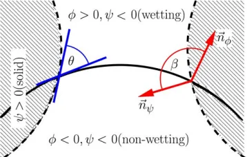
![Table A.1: Critical curvature values calculated by Mason and Morrow [33].](https://thumb-us.123doks.com/thumbv2/123dok_us/8563140.366278/31.612.128.486.264.460/table-critical-curvature-values-calculated-mason-morrow.webp)