Nystr¨om Method with Kernel K-means++ Samples as Landmarks
Dino Oglic1 2 Thomas G¨artner2
Abstract
We investigate, theoretically and empirically, the effectiveness of kernelK-means++samples as landmarks in the Nystr¨om method for low-rank approximation of kernel matrices. Previous em-pirical studies (Zhang et al.,2008;Kumar et al., 2012) observe that the landmarks obtained using (kernel)K-means clustering define a good low-rank approximation of kernel matrices. However, the existing work does not provide a theoretical guarantee on the approximation error for this ap-proach to landmark selection. We close this gap and provide the first bound on the approxima-tion error of the Nystr¨om method with kernelK -means++samples as landmarks. Moreover, for the frequently used Gaussian kernel we provide a theoretically sound motivation for performing Lloyd refinements of kernelK-means++ land-marks in the instance space. We substantiate our theoretical results empirically by comparing the approach to several state-of-the-art algorithms.
1. Introduction
We consider the problem of finding a good low-rank approx-imation for a given symmetric and positive definite matrix. Such matrices arise in kernel methods (Sch¨olkopf & Smola, 2001) where the data is often first transformed to a sym-metric and positive definite matrix and then an off-the-shelf matrix-based algorithm is used for solving classification and regression problems, clustering, anomaly detection, and dimensionality reduction (Bach & Jordan,2005). These learning problems can often be posed as convex optimiza-tion problems for which the representer theorem (Wahba, 1990) guarantees that the optimal solution can be found in the subspace of the kernel feature space spanned by the instances. To find the optimal solution in a problem withn instances, it is often required to perform a matrix inversion 1Institut f¨ur Informatik III, Universit¨at Bonn, Germany2School
of Computer Science, The University of Nottingham, United King-dom. Correspondence to: Dino Oglic<[email protected]>.
Proceedings of the34thInternational Conference on Machine Learning, Sydney, Australia, PMLR 70, 2017. Copyright 2017 by
the author(s).
or eigendecomposition which scale asO n3
. To overcome this computational shortcoming and scale kernel methods to large scale datasets,Williams & Seeger(2001) have pro-posed to use a variant of the Nystr¨om method (Nystr¨om, 1930) for low-rank approximation of kernel matrices. The approach is motivated by the fact that frequently used ker-nels have a fast decaying spectrum and that small eigen-values can be removed without a significant effect on the precision (Sch¨olkopf & Smola,2001). For a given sub-set ofl landmarks, the Nystr¨om method finds a low-rank ap-proximation in timeO l2n+l3and kernel methods with the low-rank approximation in place of the kernel matrix scale asO l3. In practice,l nand the approach can scale kernel methods to millions of instances.
2. Nystr¨om Method
In this section, we review the Nystr¨om method for low-rank approximation of kernel matrices. The method was originally proposed for the approximation of integral eigen-functions (Nystr¨om,1930) and later adopted to low-rank approximation of kernel matrices by Williams & Seeger (2001). We present it here in a slightly different light by fol-lowing the approach to subspace approximations bySmola & Sch¨olkopf(2000,2001).
Let X be an instance space and X = {x1, x2,· · ·, xn}
an independent sample from a Borel probability measure defined onX. LetHbe a reproducing kernel Hilbert space
with a positive definite kernelh:X × X → R. Given a
set of landmark pointsZ ={z1,· · ·zm}(not necessarily
a subset of the sample) the goal is to approximate kernel functionsh(xi,·)for alli= 1, nusing linear combinations
of the landmarks. This goal can be formally stated as
min
α∈Rm×n
n X i=1
h(xi,·)− m
X
j=1
αj,ih(zj,·)
2 H . (1)
LetH denote the kernel matrix over all samples and land-marks and let HZ denote the block in this matrix
corre-sponding to the kernel values between the landmarks. Addi-tionally, lethxdenote a vector with entries corresponding to
the kernel values between an instancexand the landmarks. After expanding the norm, the problem is transformed into
min
α∈Rm×n
n
X
i=1
Hii−2h>xiαi+α >
i HZαi, (2)
whereαidenotes theith column ofα. Each summand in
the optimization objective is a convex function depending only on one column ofα. Hence, the optimal solution is
α=HZ−1HZ×X.
From here it then follows that the optimal approximation ˜
HX|Zof the matrixHX using landmarksZis given by
˜
HX|Z =HX×ZHZ−1HZ×X.
While the problem of computing the optimal projections of instances to a subspace spanned by the landmarks is con-vex and solvable in closed form (see above), the problem of choosing the best set of landmarks is a combinatorial problem that is difficult to solve. To evaluate the effective-ness of the subspace spanned by a given set of landmarks it is standard to use the Schatten matrix norms (Weidmann, 1980). TheSchattenp-normof a symmetric and positive
def-inite matrixHis defined askHkp = (Pn
i=1λ
p i)
1/p ,where λi ≥ 0are eigenvalues ofH andp≥1. Forp=∞the
Schattenp-norm is equal to the operator norm and forp= 2
it is equal to the Frobenius norm. The three most frequently used Schatten norms arep= 1,2,∞and for these norms the following inequalities hold:
kHk∞= max
i λi≤
s X i λ2 i = q
tr (H>H) =kHk
2
≤X
i
λi= tr (H) =kHk1.
From Eq. (1) and (2) it follows that for a subspace spanned by a given set of landmarksZ, the1-norm approximation error of the optimal projections onto this space is given by
L(α∗) = tr(HX)−tr( ˜HX|Z) =
HX−
˜ HX|Z
1.
The latter equation follows from the properties of trace and the fact thatΞ = HX −H˜X|Z is a symmetric and
positive definite matrix withΞij = hξ(xi,·), ξ(xj,·)iH
andξ(xi,·) =h(xi,·)−P m
k=1α∗k,ih(zk,·).
For a good Nystr¨om approximation of a kernel matrix it is crucial to select the landmarks to reduce the error in one of the frequently used Schattenp-norms, i.e.,
Z∗= arg min
Z⊂span(X),|Z|=K
HX−
˜ HX|Z
p.
Let us denote withVKandΛKthe topKeigenvectors and
eigenvalues of the kernel matrixHX. Then, at the low-rank
approximationH˜∗
X|Z =VKΛKVK>, the Schattenp-norm
error attains its minimal value (Golub & van Loan,1996).
3. Kernel K-means++ Samples as Landmarks
We start with a review ofK-means clustering (Lloyd,1982) and then give the first complete proof of a claim stated inDing & He(2004) andXu et al.(2015) on the relation between the subspace spanned by the top(K−1)left sin-gular vectors of the data matrix and that spanned by optimal K-means centroids. Building on a result byArthur & Vas-silvitskii(2007) we then bound the relative approximation error in the Frobenius norm of the Nystr¨om method with kernelK-means++samples as landmarks.Let the instance spaceX ⊂Rdand letKdenote the number of clusters. InK-means clustering the goal is to choose a set of centersC={c1,· · ·, cK}minimizing the potential
φ(C) = X
x∈X
min
c∈Ckx−ck
2 = K X k=1 X
x∈Pk
kx−ckk
2
,
where Pk = {x∈X | P(x) =ck} is a clustering cell
and P: X → C denotes the centroid assignment func-tion. For a clustering cellPk the centroid is computed as
1
|Pk| P
withP ∈Rn×K thecluster indicator matrixof the
cluster-ingCsuch thatpij =1/√nj when instancexiis assigned
to centroidcj, andpij = 0otherwise. Herenjdenotes the
number of instances assigned to centroidcj. Without loss
of generality, we assume that the columns of the data matrix X ∈Rd×nare centered instances (i.e.,Pni=1xi/n= 0).
Now, using the introduced notation we can write the cluster-ing potential as (Ding & He,2004;Boutsidis et al.,2009)
φ(C) =
X−XP P>
2
2.
Denoting withpitheith column inPwe have that it holds
p>i pj =δij, whereδij = 1ifi=jand otherwiseδij = 0.
Hence, it holds thatP>P = IK andP is an orthogonal
projection matrix with rankK. LetCdenote the family of
all possible clustering indicator matrices of rankK. Then, theK-means optimization problem is equivalent to the con-strained low-rank approximation problem
P∗= arg min
P∈C
X−XP P>
2
2.
From here, using the relation between the squared Schatten 2-norm and the matrix trace we obtain
P∗= arg min
P∈C
tr X>X
−tr P>X>XP
. (3)
In the remainder of the section, we refer to the constrained optimization objective from Eq. (3) as thediscrete
prob-lem. For this problem,Ding & He(2004) observe that the set of vectors{p1,· · · , pK,e/√n}is linearly dependent (e
is a vector of ones) and that the rank of the optimization problem can be reduced. AsPK
i=1
√
nipi=e, there exists
a linear orthonormal transformation of the subspace basis given by the columns ofPsuch that one of the vectors in the new basis of the subspace spanned byPise/√n. Such
transformations are equivalent to a rotation of the subspace. Let R ∈ RK×K denote an orthonormal transformation matrix such that the vectors{pi}
K
i=1map to{qi} K i=1with
qK =√1ne. This is equivalent to requiring that theKth
col-umn inRisrK = pnn1,· · ·,pnnK
>
andq>i e= 0for i= 1, K−1. Moreover, fromQ=P RandR>R=IKit
follows that
Q>Q=R>P>P R=R>R=IK.
Hence, if we denote withQK−1the matrix-block with the
first(K−1)columns ofQthen the problem from Eq. (3) can be written as (Ding & He,2004;Xu et al.,2015)
Q∗K−1= arg max
QK−1∈Rn×(K−1)
tr Q>K−1X>XQK−1
s.t. Q>K−1QK−1=IK−1
Q=P R ∧ qK =
1
√
ne.
WhileP is an orthonormal indicator/sparse matrix of rank K,Qis a piecewise constant and in general non-sparse or-thonormal matrix of the same rank. The latter optimization problem can be relaxed by not adding the structural con-straintsQ=P RandqK =e/√n. The resulting
optimiza-tion problem is known as the Rayleigh–Ritz quotient (e.g., seeL¨utkepohl,1997) and in the remainder of the section we refer to it as thecontinuousproblem. The optimal solution
to the continuous problem is (up to a rotation of the basis) defined by the top(K−1)eigenvectors from the eigende-composition of the positive definite matrixX>Xand the optimal value of the relaxed optimization objective is the sum of the eigenvalues corresponding to this solution. As the continuous solution is (in general) not sparse, the dis-crete problem is better described with non-sparse piecewise constant matrixQthan with sparse indicator matrixP. Ding & He(2004) andXu et al.(2015) have formulated a theorem which claims that the subspace spanned by op-timalK-centroids is in fact the subspace spanned by the top (K−1)left singular vectors ofX. The proofs pro-vided in these works are, however, restricted to the case when the discrete and continuous/relaxed version of the optimization problem match. We address here this claim without that restriction and amend their formulation ac-cordingly. For this purpose, let C∗ = {c1,· · ·, cK}
be K centroids specifying an optimal K-means cluster-ing (i.e., minimizcluster-ing the potential). The between clus-ter scatclus-ter matrix S = PK
i=1nicic>i projects any vector
x∈ X to a subspace spanned by the centroid vectors, i.e., Sx = PK
i=1ni c>i x
ci ∈ span{c1,· · · , cK}. Let also
λKdenote theKth eigenvalue ofH =X>Xand assume
the eigenvalues are listed in descending order. A proof of the following proposition is provided in AppendixA. Proposition 1. Suppose that the subspace spanned by op-timalK-means centroids has a basis that consists of left singular vectors ofX. If the gap between the eigenvalues
λK−1andλKis sufficiently large (see the proof for explicit
definition), then the optimalK-means centroids and the top
(K−1)left singular vectors ofXspan the same subspace.
Proposition 2. In contrast to the claim byDing & He(2004) and Xu et al. (2015), it is possible that no basis of the subspace spanned by optimalK-means centroids consists of left singular vectors ofX. In that case, the subspace spanned by the top(K−1)left singular vectors is different from that spanned by optimalK-means centroids.
LetX=UΣV>be anSVDdecomposition ofXand denote withUK the topKleft singular vectors from this
decom-position. Let alsoUK⊥denote the dual matrix ofUK and
φ(C∗|UK)the clustering potential given by the
projec-tions ofXandC∗onto the subspaceU
K.
Proposition 3. LetHKdenote the optimal rankK
optimalK-means clustering ofX. Then, it holds
φ(C∗)≤ kH−HK−1k1+φ(C
∗|U
K−1).
Let us now relate Proposition1to the result from Section2 where we were interested in finding a set of landmarks span-ning the subspace that preserves most of the variance of the data in the kernel feature space. Assuming that the conditions from Proposition1are satisfied, the Nystr¨om approximation using optimal kernelK-means centroids as landmarks projects the data to a subspace with the highest possible variance. Hence, under these conditions optimal kernelK-means landmarks provide the optimal rank(K−1) reconstruction of the kernel matrix. However, for a kernel K-means centroid there does not necessarily exist a point in the instance space that maps to it. To account for this and the hardness of the kernelK-means clustering prob-lem (Aloise et al.,2009), we propose to approximate the centroids with kernelK-means++samples. This sampling strategy iteratively builds up a set of landmarks such that in each iteration an instance is selected with probability proportional to its contribution to the clustering potential in which previously selected instances act as cluster cen-ters. For a problem withninstances and dimensiond, the strategy selectsKlandmarks in timeO(Knd).
Before we give a bound on the Nystr¨om approximation with kernelK-means++samples as landmarks, we provide a result byArthur & Vassilvitskii(2007) on the approximation error of the optimal clustering using this sampling scheme. Theorem 4. [Arthur & Vassilvitskii(2007)] If a clustering
Cis constructed using theK-means++sampling scheme then the corresponding clustering potentialφ(C)satisfies
E[φ(C)]≤8 (lnK+ 2)φ(C∗),
whereC∗ is an optimal clustering and the expectation is taken with respect to the sampling distribution.
Having presented all the relevant results, we now give a bound on the approximation error of the Nystr¨om method with kernelK-means++samples as landmarks. A proof of the following theorem is provided in AppendixA.
Theorem 5. LetH be a kernel matrix with a finite rank factorizationH = Φ (X)>Φ (X). Denote withHK the
optimal rankK approximation of H and let H˜K be the
Nystr¨om approximation of the same rank obtained using kernelK-means++samples as landmarks. Then, it holds
E
"
kH−H˜Kk2
kH−HKk2
#
≤8(ln(K+ 1) + 2)(√n−K+ ΘK),
withΘK =φ(C
∗|U
K)/kH−HKk2, whereUKdenotes the top
Kleft singular vectors ofΦ (X)andC∗an optimal kernel
K-means clustering with(K+ 1)clusters.
Corollary 6. Whenφ(C∗|UK)≤
√
n−KkH−HKk2, then the additive termΘK ≤
√
n−Kand
E
"
kH−H˜Kk2
kH−HKk2
#
∈ OlnK√n−K. (4)
The given bound for low-rank approximation of symmetric and positive definite matrices holds for the Nystr¨om method with kernelK-means++ samples as landmarkswithout any Lloyd iterations(Lloyd,1982). To obtain even better
landmarks, it is possible to first sample candidates using the kernelK-means++sampling scheme and then attempt a Lloyd refinement in the instance space (motivation for this is provided in Section4.3). If the clustering potential is decreased as a result of this, the iteration is considered successful and the landmarks are updated. Otherwise, the refinement is rejected and current candidates are selected as landmarks. This is one of the landmark selection strategies we analyze in our experiments (e.g., see AppendixC). Let us now discuss the properties of our bound with re-spect to the rank of the approximation. From Corollary6 it follows that the bound on the relative approximation er-ror increases initially (for small K) with lnK and then decreases asKapproachesn. This is to be expected as a largerKmeans we are trying to find a higher dimensional subspace and initially this results in having to solve a more difficult problem. The bound on the low-rank approxima-tion error is, on the other hand, obtained by multiplying withkH−HKk2 which depends on the spectrum of the
kernel matrix and decreases withK. In order to be able to generalize at all, one has to assume that the spectrum falls rather sharply and typical assumptions areλi ∈ O(i−a)
witha > 1orλi ∈ O e−bi
withb > 0(e.g., see Sec-tion4.3,Bach,2013). It is simple to show that fora≥2, K >1, andλi∈ O(i−a)such falls are sharper thanlnK
(Corollary7, AppendixA). Thus, our bound on the low-rank approximation error decreases withKfor sensible choices of the kernel function. Note that a similar state-of-the-art bound on the relative approximation error byLi et al.(2016) exhibits worse behavior and grows linearly withK.
4. Discussion
We start with a brief overview of alternative approaches to landmark selection in the Nystr¨om method for low-rank approximation of kernel matrices. Following this, we fo-cus on a bound that is the most similar to ours, that of K-DPP-Nystr¨om (Li et al.,2016). Then, for the frequently
4.1. Related Approaches
As pointed in Sections1and2, the choice of landmarks is instrumental for the goodness of the Nystr¨om low-rank approximations. For this reason, the existing work on the Nystr¨om method has focused mainly on landmark selection techniques with theoretical guarantees. These approaches can be divided into four groups: i) random sampling, ii)
greedy methods,iii) methods based on the Cholesky
decom-position,iv) vector quantization (e.g.,K-means clustering). The simplest strategy for choosing the landmarks is by uni-formly sampling them from a given set of instances. This was the strategy that was proposed byWilliams & Seeger (2001) in the first paper on the Nystr¨om method for low-rank approximation of kernel matrices. Following this, more so-phisticated non-uniform sampling schemes were proposed. The schemes that received a lot of attention over the past years are the selection of landmarks by sampling propor-tional to column norms of the kernel matrix (Drineas et al., 2006), diagonal entries of the kernel matrixDrineas & Ma-honey(2005), approximate leverage scores (Alaoui & Ma-honey,2015;Gittens & Mahoney,2016), and submatrix determinants (Belabbas & Wolfe,2009; Li et al.,2016). From this group of methods, the approximate leverage score sampling and theK-DPPNystr¨om method (see Section4.2)
are considered state-of-the-art methods in low-rank approxi-mation of kernel matrices.
The second group of landmark selection techniques are greedy methods. A well-performing representative from this group is a method for sparse approximations proposed bySmola & Sch¨olkopf(2000) for which it was later inde-pendently established (Kumar et al.,2012) that it performs very well in practice—second only toK-means clustering. The third group of methods relies on the incomplete Cholesky decomposition to construct a low-rank approx-imation of a kernel matrix (Fine & Scheinberg,2002;Bach & Jordan,2005;Kulis et al.,2006). An interesting aspect of the work byBach & Jordan(2005) and that ofKulis et al. (2006) is the incorporation of side information/labels into the process of finding a good low-rank approximations of a given kernel matrix.
Beside these approaches, an influential ensemble method for low-rank approximation of kernel matrices was pro-posed byKumar et al.(2012). This work also contains an empirical study with a number of approaches to landmark selection.Kumar et al.(2012) also note that the landmarks obtained using instance spaceK-means clustering perform the best among non-ensemble methods.
4.2. K-DPP Nystr¨om Method
The first bound on the Nystr¨om approximation with land-marks sampled proportional to submatrix determinants was
given byBelabbas & Wolfe(2009).Li et al.(2016) recog-nize this sampling scheme as a determinantal point process and extend the bound to account for the case whenl land-marks are selected to make an approximation of rankK≤l. That bound can be formally specified as (Li et al.,2016)
E
"
kH−H˜Kk2
kH−HKk2
#
≤ l+ 1
l+ 1−K
√
n−K. (5)
Forl=K, the bound can be derived from that ofBelabbas & Wolfe(Theorem 1,2009) by applying the inequalities between the corresponding Schattenp-norms.
The bounds obtained byBelabbas & Wolfe(2009) andLi et al.(2016) can be directly compared to the bound from Corollary 6. From Eq. (5), forl = K+ 1, we get that the expected relative approximation error of the K-DPP
Nystr¨om method scales likeO K√n−K. For a good worst case guarantee on the generalization error of learning with Nystr¨om approximations (see, e.g.,Yang et al.,2012), the parameterK scales as √n. Plugging this parameter estimate into Eq. (4), we see that the upper bound on the ex-pected error with kernelK-means++landmarks scales like
O(√nlnn)and that withK-DPPlandmarks likeO(n).
Having compared our bound to that of K-DPPlandmark selection, we now discuss some specifics of the empirical study performed byLi et al.(2016). The crucial step of that landmark selection strategy is the ability to efficiently sample from aK-DPP. To achieve this, the authors have
pro-posed to use a Markov chain with a worst case mixing time linear in the number of instances. The mixing bound holds provided that a data-dependent parameter satisfies a condi-tion which is computacondi-tionally difficult to verify (Seccondi-tion 5, Li et al.,2016). Moreover, there are cases when this condi-tion is not satisfied and for which the mixing bound does not hold. In their empirical evaluation of theK-DPPNystr¨om
method,Li et al.(2016) have chosen the initial state of the Markov chain by sampling it using theK-means++scheme and then run the chain for100-300iterations. While the choice of the initial state is not discussed by the authors, one reason that this could be a good choice is because it starts the chain from a high density region. To verify this hypothesis, we simulate theK-DPPNystr¨om method by choosing the
4.3. Instance Space K-means Centroids as Landmarks We first address the approach to landmark selection based onK-means clustering in the instance space (Zhang et al., 2008) and then give a theoretically sound motivation for why these landmarks work well with the frequently used Gaus-sian kernel. The outlined reasoning motivates the instance space Lloyd refinements of kernelK-means++samples and it can be extended to other kernel feature spaces by following the derivations fromBurges(1999).
The only existing bound for instance spaceK-means land-marks was provided byZhang et al.(2008). However, this bound only works for kernel functions that satisfy
(h(a, b)−h(c, d))2≤η(h,X)ka−ck2− kb−dk2,
for alla, b, c, d∈ X and a data- and kernel-dependent
con-stantη(h,X). In contrast to this, our bound holds for all
kernels over Euclidean spaces. The bound given byZhang et al. (2008) is also a worst case bound, while ours is a bound in the expectation. The type of the error itself is also different, as we bound the relative error andZhang et al. (2008) bound the error in the Frobenius norm. The disad-vantage of the latter is in the sensitivity to scaling and such bounds become loose even if a single entry of the matrix is large (Li et al.,2016). Having established the difference in the type of the bounds, it cannot be claimed that one is sharper than the other. However, it is important to note that the bound byZhang et al.(Proposition 3,2008) contains the full clustering potentialφ(C∗)multiplied byn√n/Kas a
term and this is significantly larger than the rank dependent term from our bound (e.g., see Theorem5).
Burges(1999) has investigated the geometry of kernel fea-ture spaces and a part of that work refers to the Gaussian kernel. We review the results related to this kernel feature space and give an intuition for whyK-means clustering in the instance space provides a good set of landmarks for the Nystr¨om approximation of the Gaussian kernel matrix. The reasoning can be extended to other kernel feature spaces as long as the manifold onto which the data is projected in the kernel feature space is a flat Riemannian manifold with the geodesic distance between the points expressed in terms of the Euclidean distance between instances (e.g., see Riemmannian metric tensors inBurges,1999).
The frequently used Gaussian kernel is given by
h(x, y) =hΦ (x),Φ (y)i= exp kx−yk2
/2σ2,
where the feature mapΦ (x)is infinite dimensional and for a subsetX of the instance spaceX ∈ Rd also infinitely continuously differentiable onX. As inBurges(1999) we denote withS the image ofX in the reproducing kernel Hilbert space ofh. The imageS is ar ≤ddimensional surface in this Hilbert space. As noted byBurges(1999)
the imageSis a Hausdorff space (Hilbert space is a metric space and, thus, a Hausdorff space) and has a countable basis of open sets (the reproducing kernel Hilbert space of the Gaussian kernel is separable). So, for S to be a differentiable manifold (Boothby,1986) the imageSneeds
to be locally Euclidean of dimensionr≤d.
We assume that our set of instancesXis mapped to a differ-entiable manifold in the reproducing kernel Hilbert space
H. On this manifold a Riemannian metric can be defined
and, thus, the setX is mapped to a Riemannian manifoldS.
Burges(1999) has showed that the Riemannian metric ten-sor induced by this kernel feature map isgij = δσij2, where
δij = 1ifi =jand zero otherwise (1 ≤i, j ≤d). This
form of the tensor implies that the manifold is flat. From the obtained metric tensor, it follows that the squared geodesic distance between two pointsΦ (x)andΦ (y)onS
is equal to theσ-scaled Euclidean distance betweenxandy in the instance space, i.e.,dS(Φ (x),Φ (y))2=kx−yk2
/σ2.
For a clusterPk, the geodesic centroid is a point onSthat
minimizes the distance to other cluster points (centroid in theK-means sense). For our instance space, we have that
c∗k = arg min c∈Rd
X
x∈Pk
kx−ck2⇒c∗k =
1
|Pk|
X
x∈Pk x.
Thus, by doingK-means clustering in the instance space we are performing approximate geodesic clustering on the manifold onto which the data is embedded in the Gaussian kernel feature space. It is important to note here that a cen-troid from the instance space is only an approximation to the geodesic centroid from the kernel feature space – the preimage of the kernel feature space centroid does not nec-essarily exist. As the manifold is flat, geodesic centroids are ‘good’ approximations to kernelK-means centroids. Hence, by selecting centroids obtained usingK-means clustering in the instance space we are making a good estimate of the kernelK-means centroids. For the latter centroids, we know that under the conditions of Proposition1they span the same subspace as the top(K−1)left singular vectors of a finite rank factorization of the kernel matrix and, thus, define a good low-rank approximation of the kernel matrix.
5. Experiments
Having reviewed the state-of-the-art methods in select-ing landmarks for the Nystr¨om low-rank approximation of kernel matrices, we perform a series of experiments to demonstrate the effectiveness of the proposed approach and substantiate our claims from Sections 3and 4. We achieve this by comparing our approach to the state-of-the-art in landmark selection – approximate leverage score sam-pling (Gittens & Mahoney,2016) and theK-DPPNystr¨om
-16 -12 -8 -4 0 -1.
2.3 5.6 8.9 12.2
logγ
log
lift
(a) ailerons
kernelK-means++ leverage scores (uniform sketch) K-DPP(1 000MCsteps) kernelK-means++(with restarts) leverage scores (K-diagonal sketch) K-DPP(10 000MCsteps)
-16 -12 -8 -4 0 -0.5
0.6 1.7 2.8 3.9
logγ
(b) parkinsons
-13.2 -9.9 -6.6 -3.3 0. -0.5
2.9 6.3 9.7 13.1
logγ
(c) elevators
-23.2 -17.4 -11.6 -5.8 0. -0.2
0. 0.2 0.4 0.6
logγ
(d) ujil
-13.2 -9.9 -6.6 -3.3 0. -0.5
1.2 2.9 4.6 6.3
logγ
[image:7.612.60.540.64.195.2](e) cal-housing
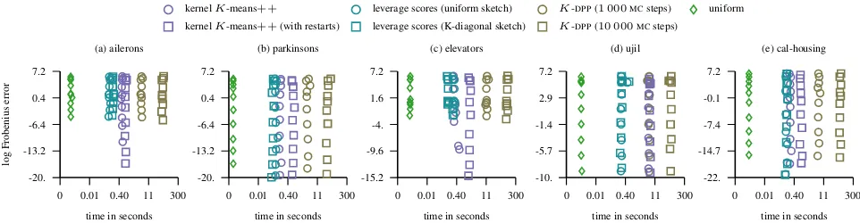
Figure 1.The figure shows the lift of the approximation error in the Frobenius norm as the bandwidth parameter of the Gaussian kernel varies and the approximation rank is fixed toK= 100. The lift of a landmark selection strategy indicates how much better it is to approximate the kernel matrix with landmarks obtained using that strategy compared to the uniformly sampled ones.
0 0.01 0.40 11 300 -20.
-13.2 -6.4 0.4 7.2
time in seconds
log
Frobenius
error
(a) ailerons
kernelK-means++ leverage scores (uniform sketch) K-DPP(1 000MCsteps) uniform kernelK-means++(with restarts) leverage scores (K-diagonal sketch) K-DPP(10 000MCsteps)
0 0.01 0.40 11 300 -20.
-13.2 -6.4 0.4 7.2
time in seconds (b) parkinsons
0 0.01 0.40 11 300 -15.2
-9.6 -4. 1.6 7.2
time in seconds (c) elevators
0 0.01 0.40 11 300 -10.
-5.7 -1.4 2.9 7.2
time in seconds (d) ujil
0 0.01 0.40 11 300 -22.
-14.7 -7.4 -0.1 7.2
time in seconds (e) cal-housing
Figure 2.The figure shows the time it takes to select landmarks via different schemes together with the corresponding error in the Frobenius norm while the bandwidth of the Gaussian kernel varies and the approximation rank is fixed toK= 100.
Before we present and discuss our empirical results, we provide a brief summary of the experimental setup. The experiments were performed on13real-world datasets avail-able at theUCIandLIACCrepositories. Each of the selected
datasets consists of more than 5 000instances. Prior to running the experiments, the datasets were standardized to have zero mean and unit variance. We measure the good-ness of a landmark selection strategy with the lift of the approximation error in the Frobenius norm and the time needed to select the landmarks. The lift of the approxima-tion error of a given strategy is computed by dividing the error obtained by sampling landmarks uniformly without replacement (Williams & Seeger,2001) with the error of the given strategy. In contrast to the empirical study byLi et al.(2016), we do not perform any sub-sampling of the datasets with less than25 000instances and compute the Frobenius norm error using full kernel matrices. On one larger dataset with more than25 000instances the memory requirements were hindering our parallel implementation and we, therefore, subsampled it to25 000instances ( ct-slicedataset, AppendixC). By performing our empirical
study on full datasets, we are avoiding a potentially negative influence of the sub-sampling on the effectiveness of the compared landmark selection strategies, time consumed,
and the accuracy of the approximation error. Following pre-vious empirical studies (Drineas & Mahoney,2005;Kumar et al.,2012;Li et al.,2016), we evaluate the goodness of landmark selection strategies using the Gaussian kernel and repeat all experiments10times to account for their non-deterministic nature. We refer toγ=1/σ2as the bandwidth
[image:7.612.58.539.249.374.2]princi-5 10 25 50 100 -0.2
1.6 3.4 5.2 7.
rank
log
lift
(a) ailerons
kernelK-means++ leverage scores (uniform sketch) K-DPP(1 000MCsteps) kernelK-means++(with restarts) leverage scores (K-diagonal sketch) K-DPP(10 000MCsteps)
5 10 25 50 100 -0.2
0.8 1.8 2.8 3.8
rank (b) parkinsons
5 10 25 50 100 -0.2
1.5 3.2 4.9 6.6
rank (c) elevators
5 10 25 50 100 -0.8
-0.5 -0.2 0.1 0.4
rank (d) ujil
5 10 25 50 100 -0.4
0.9 2.2 3.5 4.8
[image:8.612.57.539.64.194.2]rank (e) cal-housing
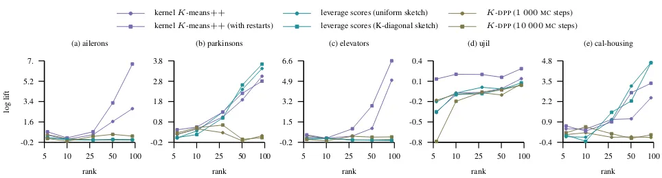
Figure 3.The figure shows the improvement in the lift of the approximation error measured in the Frobenius norm that comes as a result of the increase in the rank of the approximation. The bandwidth parameter of the Gaussian kernel is set to the inverse of the squared median pairwise distance between the samples.
pal part of the spectral mass is concentrated at the top100 eigenvalues and we set the approximation rankK = 100. Figure1demonstrates the effectiveness of evaluated selec-tion strategies as the bandwidth varies. More precisely, as the log value of the bandwidth parameter approaches to zero the kernel matrix is close to being the identity matrix, thus, hindering low-rank approximations. In contrast to this, as the bandwidth value gets smaller the spectrum mass be-comes concentrated in a small number of eigenvalues and low-rank approximations are more accurate. Overall, the kernelK-means++ sampling scheme performs the best across all13datasets. It is the best performing method on 10of the considered datasets and a competitive alternative on the remaining ones. The improvement over alternative approaches is especially evident on datasetsaileronsand elevators. The approximate leverage score sampling is on
most datasets competitive and achieves a significantly better approximation than alternatives on the datasetcal-housing.
The approximations for theK-DPPNystr¨om method with
10 000 MCsteps are more accurate than that with1 000 steps. The low lift values for that method seem to indicate that the approach moves rather slowly away from the ini-tial state sampled uniformly at random. This choice of the initial state is the main difference in the experimental setup compared to the study byLi et al.(2016) where theK-DPP
chain was initialized withK-means++sampling scheme. Figure2depicts the runtime costs incurred by each of the sampling schemes. It is evident that compared to other methods the cost of running the K-DPP chain with uni-formly chosen initial state for more than1 000steps results in a huge runtime cost without an appropriate reward in the accuracy. From this figure it is also evident that the approxi-mate leverage score and kernelK-means++sampling are efficient and run in approximately the same time apart from the datasetujil(see alsoct-slice, AppendixC). This dataset
has more than500attributes and it is time consuming for the kernelK-means++sampling scheme (our implementa-tion does not cache/pre-compute the kernel matrix). While
on such large dimensional datasets the kernelK-means++ sampling scheme is not as fast as the approximate lever-age score sampling, it is still the best performing landmark selection technique in terms of the accuracy.
In Figure3we summarize the results of the second exper-iment where we compare the improvement in the approxi-mation achieved by each of the methods as the rank of the approximation is increased from5to100. The results indi-cate that the kernelK-means++sampling achieves the best increase in the lift of the approximation error. On most of the datasets the approximate leverage score sampling is com-petitive. That method also performs much better than the K-DPPNystr¨om approach initialized via uniform sampling.
Acknowledgment:We are grateful for access to the Univer-sity of Nottingham High Performance Computing Facility.
References
Alaoui, Ahmed E. and Mahoney, Michael W. Fast randomized kernel ridge regression with statistical guarantees. InAdvances in Neural Information Processing Systems 28, 2015.
Aloise, Daniel, Deshpande, Amit, Hansen, Pierre, and Popat, Preyas. NP-hardness of Euclidean sum-of-squares clustering.
Machine Learning, 2009.
Arthur, David and Vassilvitskii, Sergei. K-means++: The ad-vantages of careful seeding. InProceedings of the Eighteenth Annual ACM-SIAM Symposium on Discrete Algorithms, 2007.
Bach, Francis R. Sharp analysis of low-rank kernel matrix approx-imations. InProceedings of the 26th Annual Conference on Learning Theory, 2013.
Bach, Francis R. and Jordan, Michael I. Predictive low-rank decomposition for kernel methods. InProceedings of the 22nd International Conference on Machine Learning, 2005.
Belabbas, Mohamed A. and Wolfe, Patrick J. Spectral methods in machine learning: New strategies for very large datasets.
Proceedings of the National Academy of Sciences of the USA,
2009.
Boothby, William M.An introduction to differentiable manifolds and Riemannian geometry. Academic Press, 1986.
Boutsidis, Christos, Drineas, Petros, and Mahoney, Michael W. Unsupervised feature selection for the K-means clustering prob-lem. InAdvances in Neural Information Processing Systems 22,
2009.
Burges, Christopher J. C. Geometry and invariance in kernel based methods. InAdvances in Kernel Methods. MIT Press, 1999.
Ding, Chris and He, Xiaofeng. K-means clustering via principal component analysis. InProceedings of the 21st International Conference on Machine Learning, 2004.
Drineas, Petros and Mahoney, Michael W. On the Nystr¨om method for approximating a Gram matrix for improved kernel-based learning.Journal of Machine Learning Research, 2005.
Drineas, Petros, Kannan, Ravi, and Mahoney, Michael W. Fast Monte Carlo algorithms for matrices II: Computing a low-rank approximation to a matrix.SIAM Journal on Computing, 2006.
Fine, Shai and Scheinberg, Katya. Efficient SVM training using low-rank kernel representations.Journal of Machine Learning Research, 2002.
Gittens, Alex and Mahoney, Michael W. Revisiting the Nystr¨om method for improved large-scale machine learning. Journal Machine Learning Research, 2016.
Golub, Gene H. and van Loan, Charles F.Matrix Computations.
Johns Hopkins University Press, 1996.
Kanungo, Tapas, Mount, David M., Netanyahu, Nathan S., Piatko, Christine D., Silverman, Ruth, and Wu, Angela Y. A local search approximation algorithm for K-means clustering. In
Proceedings of the Eighteenth Annual Symposium on Computa-tional Geometry, 2002.
Kulis, Brian, Sustik, M´aty´as, and Dhillon, Inderjit. Learning low-rank kernel matrices. InProceedings of the 23rd International Conference on Machine Learning, 2006.
Kumar, Sanjiv, Mohri, Mehryar, and Talwalkar, Ameet. Sampling methods for the Nystr¨om method.Journal of Machine Learning Research, 2012.
Li, Chengtao, Jegelka, Stefanie, and Sra, Suvrit. Fast DPP sam-pling for Nystr¨om with application to kernel methods. In
Proceedings of the 33rd International Conference on Machine Learning, 2016.
Lloyd, Stuart. Least squares quantization in PCM.IEEE Transac-tions on Information Theory, 1982.
L¨utkepohl, Helmut.Handbook of Matrices. Wiley, 1997.
Nystr¨om, Evert J. ¨Uber die praktische Aufl¨osung von Integral-gleichungen mit Anwendungen auf Randwertaufgaben. Acta Mathematica, 1930.
Sch¨olkopf, Bernhard and Smola, Alexander J. Learning with kernels: Support vector machines, regularization, optimization, and beyond. MIT Press, 2001.
Smola, Alexander J. and Sch¨olkopf, Bernhard. Sparse greedy matrix approximation for machine learning. InProceedings of the 17th International Conference on Machine Learning, 2000.
Wahba, Grace.Spline models for observational data. SIAM, 1990.
Weidmann, Joachim.Linear operators in Hilbert spaces.
Springer-Verlag, 1980.
Williams, Christopher K. I. and Seeger, Matthias. Using the Nystr¨om method to speed up kernel machines. InAdvances in Neural Information Processing Systems 13. 2001.
Xu, Qin, Ding, Chris, Liu, Jinpei, and Luo, Bin. PCA-guided search for K-means.Pattern Recognition Letters, 2015.
Yang, Tianbao, Li, Yu-feng, Mahdavi, Mehrdad, Jin, Rong, and Zhou, Zhi-Hua. Nystr¨om method vs random Fourier features: A theoretical and empirical comparison. InAdvances in Neural Information Processing Systems 25. 2012.
Zhang, Kai, Tsang, Ivor W., and Kwok, James T. Improved Nystr¨om low-rank approximation and error analysis. In Proceed-ings of the 25th International Conference on Machine Learning,
A. Proofs
Lemma A.1. [Kanungo et al.(2002)] Letcbe the centroid of a clusterCwithninstances and letz be an arbitrary point fromRd. Then, it holds
X
x∈C
kx−zk2−X
x∈C
kx−ck2=nkc−zk2.
Proof. After expanding the sums we obtain
X
x∈C
kxk2+nkzk2−2X
x∈C
hx, zi −X
x∈C
kxk2−nkck2
+ 2X
x∈C
hc, xi=nkck2+nkzk2−2nhc, zi.
We can now rewrite the latter equation as
−2nhc, zi −nkck2+ 2nkck2=nkck2−2nhc, zi,
and the claim follows from here.
Proposition 1. Suppose that the subspace spanned by op-timalK-means centroids has a basis that consists of left singular vectors ofX. If the gap between the eigenvalues
λK−1andλKis sufficiently large (see the proof for explicit
definition), then the optimalK-means centroids and the top
(K−1)left singular vectors ofXspan the same subspace.
Proof. Let M ∈ Rd×K with centroids {c
1, c2, . . . , cK}
as columns and letN = diag (n1, n2,· · ·, nK)whereni
denotes the size of the cluster with centroidci.
Now, observe thatM =XP N−1/2and that we can write
the non-constant term from Eq. (3) as
tr P>X>XP
= trN12M>M N 1 2
=
tr M N M>
= tr
K
X
i=1
nicic>i
!
.
(6)
An optimal solution ofK-means clustering places centroids to maximize this objective. From the relaxed version of the problem (described in Section3) we know that it holds
tr
K
X
i=1
nicic>i
! ≤
K−1
X
i=1
λi,
where{λi} K−1
i=1 are the top eigenvalues of the
eigendecom-positionXX>=UΛU>, andλ1≥λ2≥ · · · ≥λd≥0.
From theSVDdecompositionX =UΣV>it follows that X = Pr
i=1σiuiv>i , where ris the rank of X andr ≤
min(d−1, n−1)(note thatXis a centered data matrix). Hence,U ∈Rd×ris an orthonormal basis of the data span and we can express the centroids in this basis asM =UΓ, whereΓ = [γ1γ2 · · · γK]andγi∈Rrfori= 1, K.
Having expressed the centroids in the U-basis it is now possible to rewrite the optimization objective in this basis, as well. In particular, it holds
tr M N M>= tr UΓNΓ>U>=
tr ΓNΓ>
= tr
K
X
i=1
niγiγ>i
! = K X i=1 ni r X j=1
γji2 =
r X j=1 K X i=1
niγ2ji.
(7)
From theSVDdecomposition ofXit is possible to compute the projections of instances onto the left singular vectors, and thus retrieve the coefficient matrixΓ. For instance, projecting the data over a left singular vectorujwe get
u>jX =σjvj>,
wherevjis thejth right singular vector ofX.
Hence, the centroidciof a cluster cellPican be expressed
inU-basis by setting
γji=
σj
ni
X
l∈Pi vlj
and
niγ2ji=λjni
P
l∈Pivlj ni
2
=λjniδ2ji,
whereδji=
P
l∈Pivlj/ni. From here it then follows that
tr M N M>
= r X j=1 λj K X i=1
niδji2. (8)
As the data matrixX is centered, i.e., n1Pn
i=1xi = 0, it
follows that the columns of matrixMare linearly dependent. In particular, we have that it holds
K
X
i=1
ni
nci= 1 n
n
X
i=1
xi= 0.
From here it follows that we can express one column (e.g., centroidcK) as a linear combination of the others. Thus,
the rank of M is at most K −1 ≤ r. As the rank of span{c1, c2,· · ·, cK}is at mostK−1, then by the
assump-tion of the proposiassump-tion there are at leastr−K+ 1columns ofU that are orthogonal to this span. What this means is that in matrixΓ∈Rr×Kthere are at least(r−K+ 1)rows
with all entries equal to zero.
From the Cauchy–Schwartz inequality and the fact that right singular vectors ofXare unitary orthogonal vectors it follows that
niδji2 ≤
X
l∈Pi
On the one hand, from this inequality we can conclude that δji≤1/√ni. On the other hand, summing the first part of
the inequality over1≤i≤Kwe obtain
K
X
i=1
niδji2 ≤ K
X
i=1
X
l∈Pi
vlj2 =kvjk2= 1.
Now, in order to minimize the objective in Eq. (3) one needs to maximize the objective in Eq. (7). In other words, the rows inΓ that correspond to low value terms in Eq. (8) need to be set to zero. As λjP
K
i=1niδji2 ≤ λj it is a
good strategy to set to zero the rows that correspond to eigenvaluesλj withj ≥K, i.e.,γji =δji = 0forK ≤
j≤rand1≤i≤K.
Let us now investigate whether and when the optimal value of the relaxed objective,PK−1
j=1 λj, is attained. By applying
LemmaA.1withz= 0to Eq. (8) we obtain
r X j=1 λj K X i=1
niδji2 = r X j=1 λj K X i=1 X
l∈Pi
vlj2 −(vlj−δji)
2
=
r
X
j=1
λj 1− K
X
i=1
X
l∈Pi
(vlj−δji)
2
!
.
The maximal value of this objective is attained when the topK−1right singular vectorsV are piecewise constant over clusters. In particular, for vlj = δjiwhen l ∈ Pi,
1≤i≤K, and1≤j≤K−1the expression attains the maximal value of the continuous version of the problem,
PK−1
j=1 λj. Thus, in this case the solutions to the discrete
and continuous version of theK-means optimization prob-lem match. However, right singular vectors ofX are not necessarily piecewise constant but a perturbation of these. Takingv˜j to be the column vector with entriesv˜lj =δji
whenl∈ Piand1≤i≤K, we can write Eq. (7) as
tr M N M>=
r
X
j=1
λj
1− kvj−˜vjk
2
.
Let VK−1 be the matrix with top (K−1) right
sin-gular vectors of X. Let {u1,· · ·, uK−2, uK−1} and
{u1,· · ·, uK−2, uK} be the subspaces spanned by
cen-troids of clusteringsCK(1)andCK(2), respectively. For these two clusterings, let V˜1and V˜2 be the piecewise constant approximations to corresponding right singular vectors. In the case whenV˜16=VK−1, the gap between eigenvalues λK−1 andλK needs to be sufficiently large so that the
choice of rowsγji6= 0and1≤j≤K−1corresponds to
an optimalK-means clustering and that the corresponding centroid subspace is spanned by the top(K−1)left singular vectors ofX. In particular, it needs to hold
λK−1(1− kvK−1−v˜ (1)
K−1k 2)> λ
K(1− kvK−v˜
(2)
K k
2),
wherevjand˜v
(·)
j denote corresponding columns in matrices
VK−1andV˜·, respectively. This is equivalent to
λK−1−λK
λK−1
>
vK−1−˜v
(1)
K−1
2
− vK−˜v
(2) K 2 1− vK−v˜
(2) K 2 .
The claim follows by noting that from
0<
K
X
i=1
niδji2 = K
X
i=1
X
l∈Pi
v2lj−(vlj−δji)
2
,
it follows that
kvj−˜vjk
2
<1,
for any selected/non-zero row in matrixΓ.
Having established the condition on eigenvalues, let us now check whether the upper bound on the objective in Eq. (7) is attained when the right singular vectors are not piecewise constant. From the Cauchy-Schwarz inequality in Eq. (9), it follows that the equality is attained whenvlj = const.for
alll ∈ Pi and1 ≤i≤K. According to the assumption,
the right singular vectors are not piecewise constant and we then have the strict inequality in Eq. (9). This implies that for sufficiently large gap between the eigenvaluesλK−1and
λK, it holds
tr M N M>
=
K−1
X j=1 λj K X i=1
niδ2ji< K−1
X
j=1
λj.
Hence, in this case the optimal value of the relaxed objective is not attained.
Proposition 3. LetHKdenote the optimal rankK
approx-imation of the Gram matrixH =X>X and letC∗be an
optimalK-means clustering ofX. Then, it holds
φ(C∗)≤ kH−HK−1k1+φ(C
∗|U
K−1).
Proof. Using the notation from the proof of Proposition1,
φ(C∗) = tr X>X
−tr P>X>XP
=
r
X
j=1
λj− r
X
j=1
λj 1− K
X
i=1
X
l∈Pi
(vlj−δji)
2 ! = r X j=1 λj K X i=1 X
l∈Pi
(vlj−δji)2 .
Now, observe that
0≤δ2ji ⇐⇒ niδji2 ≤2δji
X
l∈Pi vlj
⇐⇒ X
l∈Pi
(vlj−δji)
2
≤X
Hence, we have that it holds
φ C∗|UK⊥−1
=
r
X
j=K
λj K
X
i=1
X
l∈Pi
(vlj−δji)2
≤
r
X
j=K
λj K
X
i=1
X
l∈Pi vlj2 =
r
X
j=K
λj
=kH−HK−1k1 .
The claim follows by combining the latter inequality with the fact that
φ(C∗|UK−1) =
K−1
X j=1 λj K X i=1 X
l∈Pi
(vlj−δji)2 .
Theorem 5. LetH be a kernel matrix with a finite rank factorizationH = Φ (X)>Φ (X). Denote withHK the
optimal rankK approximation of H and let H˜K be the
Nystr¨om approximation of the same rank obtained using kernelK-means++samples as landmarks. Then, it holds
E
"
kH−H˜Kk2
kH−HKk2
#
≤8(ln(K+ 1) + 2)(√n−K+ ΘK),
withΘK =φ(C
∗|U
K)/kH−HKk2, whereUKdenotes the top
Kleft singular vectors ofΦ (X)andC∗an optimal kernel
K-means clustering with(K+ 1)clusters.
Proof. Let us assume that(K+ 1)landmarks,Z⊂X, are selected using the kernelK-means++sampling scheme. Then, for the clustering potential defined withZwe have that it holds
φ(Z) =
n
X
i=1
min
z∈ZkΦ (xi)−Φ (z)k
2
≥ min
α∈R(K+1)×n
n X i=1
Φ (xi)− K+1
X
j=1
αjiΦ (zj)
2 = H− ˜ HK 1 ,
where H˜K is the Nystr¨om approximation matrix (e.g., see Section 2) of rankK defined with landmarks Z =
{z1, . . . , zK+1}andΦ (x)is the image of instancexin the
factorization space. The latter inequality follows from the fact that the distance of a point to its orthogonal projection ontospan{Φ (z1), . . . ,Φ (zK+1)}is not greater than the
distance between that point and the closest landmark from
{Φ (z1), . . . ,Φ (zK+1)}.
Now, combining this result with Proposition3and Theo-rem4, we deduce
E
h
kH−H˜Kk1
i
≤E[φ(Z)]≤8 (ln(K+ 1) + 2)φ(C∗)
≤8 (ln (K+ 1) + 2) (kH−HKk1+φ(C
∗ |U
K)).
From this and the Schattenp-norm inequalities,
kH−HKk1≤
√
n−KkH−HKk2 ∧ kHk2≤ kHk1,
we obtain the following bound
E
h
kH−H˜Kk2
i ≤
8(ln(K+ 1) + 2)(√n−KkH−HKk2+φ(C∗|UK)).
The result follows after division withkH−HKk2.
Corollary 7. Assume that the conditions of Theorem5and Corollary6are satisfied together withλi ∈ O(i−a)and
a ≥ 2. The low-rank approximation error in the Frobe-nius norm of the Nystr¨om method with kernelK-means++
samples as landmarks decreases withK >1.
Proof. First observe that
n
X
l=K
1 l2a =
1 K2a
n
X
l=K
1
(l/K)2a =
1 K2a
n−K
X
l=0
1
(1 +l/K)2a <
1 K2a
n−K
X
l=0
1
(1 +l/K)2 <
1 K2(a−1)
n−K
X
l=0
1
(1 +l)2 <
1 K2(a−1)
X
l≥0
1
(1 +l)2 ∈ O
1
K2(a−1)
.
Hence, we have that the approximation error in the Frobe-nius norm of the optimal rankKsubspace satisfies
kH−HKk2∈ O
1
(K+ 1)a−1
!
.
From here it then follows that the low-rank approximation error in Frobenius norm of the Nystr¨om method with kernel K-means++samples as landmarks satisfies
H− ˜ HK 2∈ O
√
n−K(ln (K+ 1) + 1)
(K+ 1)a−1
!
.
The claim follows by observing that fora≥2the function
ln(K+1)/(K+1)a−1decreases withK >1.
B. Addendum
Proposition 2. In contrast to the claim byDing & He(2004) and Xu et al. (2015), it is possible that no basis of the subspace spanned by optimalK-means centroids consists of left singular vectors ofX. In that case, the subspace spanned by the top(K−1)left singular vectors is different from that spanned by optimalK-means centroids.
Proof. If no basis ofspan{c1, c2, . . . , cK}is given by a
the proof of Proposition1) there are at leastKrows with non-zero entries in matrixΓ. Let us now show that this is indeed possible. The fact that a left singular vectorui is
orthogonal to the span is equivalent to
∀β∈RK: 0 =u>i
K
X
j=1
βjcj
=
u>i
K
X
j=1
r
X
l=1
βjδljσlul
=
K
X
j=1
βjσiδij= K
X
j=1
βjσi
1 nj
X
l∈Pj vli,
whereviis theith right singular vector. As the latter
equa-tion holds for all vectors β = (β1, . . . , βK) ∈ RK, the claimui⊥span{c1, . . . , cK}is equivalent to
X
l∈Pj
vli= 0 (∀j= 1, . . . , K). (10)
Moreover, as the data matrix is centered vectorvialso
satis-fiesv>i e= 0.
To construct a problem instance where no basis of the sub-space spanned by optimalK-means centroids consists of left singular vectors, we take a unit vectorvrsuch that, for
any cluster in any clustering, none of the conditions from Eq. (10) is satisfied. Then, we can construct a basis of right singular vectors using the Gram–Schmidt orthogonalization method. For instance, we can take ˜vwith ˜vi = −2i for
1≤i < nandv˜n = 2n−2, and then setvr=v˜/k˜vk, where ris the rank of the problem. Once we have constructed a right singular basis that contains vectorvr, we pick a small
positive real number as the singular value corresponding to vectorvrand select the remaining singular values so that
there are sufficiently large gaps between them (e.g., see the proof of Proposition1). By choosing a left singular basis of rankr, we form a data matrixX and the subspace spanned by optimalK-means centroids in this problem instance is not the one spanned by the top(K−1)left singular vectors. To see this, note that from Eq. (10) and the definition ofvr
it follows thatur6⊥span{c1, . . . , cK}.
Having shown that an optimal centroid subspace of data matrixX is not the one spanned by the top(K−1)left singular vectors, let us now show that there is no basis for this subspace consisting of left singular vectors. For simplicity, let us takeK = 2. According to our assump-tionσ1 σ2 σr−1 σr. Now, from Eq. (8) it
fol-lows that the largest reduction in the clustering potential is obtained by partitioning data so that the centroids for the top components are far away from the zero-vector. As the basis of span{c1, c2} consists of one vector and as
ur6⊥span{c1, c2}it then follows that the basis vector is
given byPr
j=1βjujwithβj ∈Rand at leastβ1, βr6= 0.
Hence, forK = 2and data matrixX there is no basis of span{c1, c2}that consists of a left singular vector.
C. Additional Figures
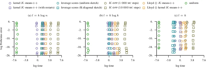
In this appendix, we provide the detailed results of our empirical study. The appendix is organized such that the results are presented by datasets that are listed in ascending order with respect to the number of instances and dimension. The empirical study provided below compares the following approaches:i) uniform sampling of landmarks,ii) approximate leverage score
sampling with uniform sketch matrix,iii) approximate leverage score sampling with the sketch matrix selected by sampling
instances proportional to the diagonal entries in the kernel matrix,iv)K-DPPNystr¨om method with1 000and10 000MC
steps and the initial state chosen by sampling landmarks uniformly at random,v)K-means clustering in the input space (Lloyd⊕K-means++),vi) kernelK-means++sampling,vii) kernelK-means++sampling with restarts,viii) kernel
K-means++sampling with restarts and Lloyd refinements in the instance space (Lloyd⊕kernelK-means++).
C.1. Parkinsons
The number of instances in this dataset isn= 5 875and the dimension of the problem isd= 21.
-16 -12 -8 -4 0 -0.5
0.6 1.7 2.8 3.9
logγ
log
lift
(a)l=klogn
kernelK-means++ leverage scores (uniform sketch) K-DPP(1 000MCsteps) Lloyd⊕K-means++ kernelK-means++(with restarts) leverage scores (K-diagonal sketch) K-DPP(10 000MCsteps) Lloyd⊕kernelK-means++
-16 -12 -8 -4 0 -0.5
0.6 1.7 2.8 3.9
logγ
(b)l=klogk
-16 -12 -8 -4 0 -0.5
0.6 1.7 2.8 3.9
logγ
[image:14.612.76.512.238.381.2](c)l=k
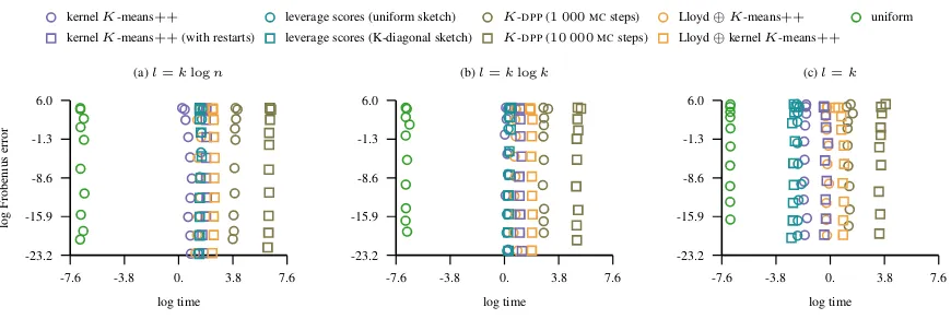
Figure 4.The figure shows the lift of the approximation error in the Frobenius norm as the bandwidth parameter of the Gaussian kernel varies and the approximation rank is fixed toK= 100. The lift of a landmark selection strategy indicates how much better it is to approximate the kernel matrix with landmarks obtained using this strategy compared to the uniformly sampled ones.
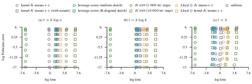
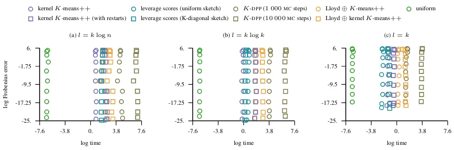
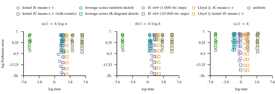
-7.6 -3.8 0. 3.8 7.6 -23.2
-15.9 -8.6 -1.3 6.0
log time
log
Frobenius
error
(a)l=klogn
kernelK-means++ leverage scores (uniform sketch) K-DPP(1 000MCsteps) Lloyd⊕K-means++ uniform kernelK-means++(with restarts) leverage scores (K-diagonal sketch) K-DPP(10 000MCsteps) Lloyd⊕kernelK-means++
-7.6 -3.8 0. 3.8 7.6 -23.2
-15.9 -8.6 -1.3 6.0
log time (b)l=klogk
-7.6 -3.8 0. 3.8 7.6 -23.2
-15.9 -8.6 -1.3 6.0
log time (c)l=k
[image:14.612.81.516.443.589.2]C.2. Delta-ailerons
The number of instances in this dataset isn= 7 129and the dimension of the problem isd= 5.
-10 -7.5 -5 -2.5 0 -0.5
0.6 1.7 2.8 3.9
logγ
log
lift
(a)l=klogn
kernelK-means++ leverage scores (uniform sketch) K-DPP(1 000MCsteps) Lloyd⊕K-means++ kernelK-means++(with restarts) leverage scores (K-diagonal sketch) K-DPP(10 000MCsteps) Lloyd⊕kernelK-means++
-10 -7.5 -5 -2.5 0 -0.5
0.6 1.7 2.8 3.9
logγ
(b)l=klogk
-10 -7.5 -5 -2.5 0 -0.5
0.6 1.7 2.8 3.9
logγ
[image:15.612.75.514.107.254.2](c)l=k
Figure 6.The figure shows the lift of the approximation error in the Frobenius norm as the bandwidth parameter of the Gaussian kernel varies and the approximation rank is fixed toK= 100. The lift of a landmark selection strategy indicates how much better it is to approximate the kernel matrix with landmarks obtained using this strategy compared to the uniformly sampled ones.
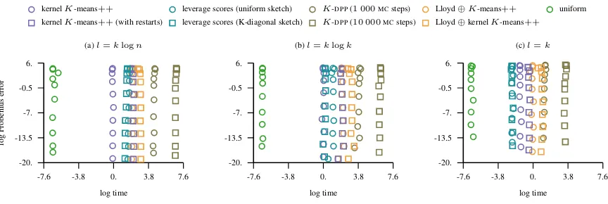
-7.6 -3.8 0. 3.8 7.6 -26.
-18. -10. -2. 6.
log time
log
Frobenius
error
(a)l=klogn
kernelK-means++ leverage scores (uniform sketch) K-DPP(1 000MCsteps) Lloyd⊕K-means++ uniform kernelK-means++(with restarts) leverage scores (K-diagonal sketch) K-DPP(10 000MCsteps) Lloyd⊕kernelK-means++
-7.6 -3.8 0. 3.8 7.6 -26.
-18. -10. -2. 6.
log time (b)l=klogk
-7.6 -3.8 0. 3.8 7.6 -26.
-18. -10. -2. 6.
log time (c)l=k
[image:15.612.82.513.316.460.2]C.3. Kinematics
The number of instances in this dataset isn= 8 192and the dimension of the problem isd= 8.
-10 -7.5 -5 -2.5 0 -0.5
-0.25 0. 0.25 0.5
logγ
log
lift
(a)l=klogn
kernelK-means++ leverage scores (uniform sketch) K-DPP(1 000MCsteps) Lloyd⊕K-means++ kernelK-means++(with restarts) leverage scores (K-diagonal sketch) K-DPP(10 000MCsteps) Lloyd⊕kernelK-means++
-10 -7.5 -5 -2.5 0 -0.5
-0.25 0. 0.25 0.5
logγ
(b)l=klogk
-10 -7.5 -5 -2.5 0 -0.5
-0.25 0. 0.25 0.5
logγ
[image:16.612.74.513.108.254.2](c)l=k
Figure 8.The figure shows the lift of the approximation error in the Frobenius norm as the bandwidth parameter of the Gaussian kernel varies and the approximation rank is fixed toK= 100. The lift of a landmark selection strategy indicates how much better it is to approximate the kernel matrix with landmarks obtained using this strategy compared to the uniformly sampled ones.
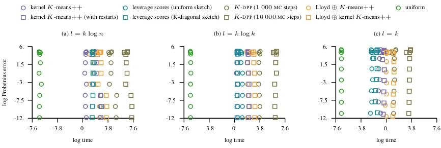
-7.6 -3.8 0. 3.8 7.6 -17.
-11.25 -5.5 0.25 6.
log time
log
Frobenius
error
(a)l=klogn
kernelK-means++ leverage scores (uniform sketch) K-DPP(1 000MCsteps) Lloyd⊕K-means++ uniform kernelK-means++(with restarts) leverage scores (K-diagonal sketch) K-DPP(10 000MCsteps) Lloyd⊕kernelK-means++
-7.6 -3.8 0. 3.8 7.6 -17.
-11.25 -5.5 0.25 6.
log time (b)l=klogk
-7.6 -3.8 0. 3.8 7.6 -17.
-11.25 -5.5 0.25 6.
log time (c)l=k
[image:16.612.76.518.313.461.2]C.4.CPU-activity
The number of instances in this dataset isn= 8 192and the dimension of the problem isd= 21.
-15.2 -11.4 -7.6 -3.8 0. -0.5
0.6 1.7 2.8 3.9
logγ
log
lift
(a)l=klogn
kernelK-means++ leverage scores (uniform sketch) K-DPP(1 000MCsteps) Lloyd⊕K-means++ kernelK-means++(with restarts) leverage scores (K-diagonal sketch) K-DPP(10 000MCsteps) Lloyd⊕kernelK-means++
-15.2 -11.4 -7.6 -3.8 0. -0.5
0.6 1.7 2.8 3.9
logγ
(b)l=klogk
-15.2 -11.4 -7.6 -3.8 0. -0.5
0.6 1.7 2.8 3.9
logγ
[image:17.612.74.513.107.254.2](c)l=k
Figure 10.The figure shows the lift of the approximation error in the Frobenius norm as the bandwidth parameter of the Gaussian kernel varies and the approximation rank is fixed toK= 100. The lift of a landmark selection strategy indicates how much better it is to approximate the kernel matrix with landmarks obtained using this strategy compared to the uniformly sampled ones.
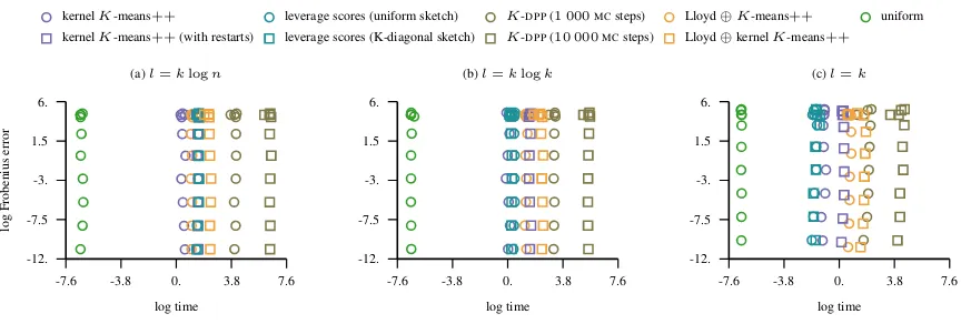
-7.6 -3.8 0. 3.8 7.6 -20.
-13.5 -7. -0.5 6.
log time
log
Frobenius
error
(a)l=klogn
kernelK-means++ leverage scores (uniform sketch) K-DPP(1 000MCsteps) Lloyd⊕K-means++ uniform kernelK-means++(with restarts) leverage scores (K-diagonal sketch) K-DPP(10 000MCsteps) Lloyd⊕kernelK-means++
-7.6 -3.8 0. 3.8 7.6 -20.
-13.5 -7. -0.5 6.
log time (b)l=klogk
-7.6 -3.8 0. 3.8 7.6 -20.
-13.5 -7. -0.5 6.
log time (c)l=k
[image:17.612.82.514.316.461.2]C.5. Bank
The number of instances in this dataset isn= 8 192and the dimension of the problem isd= 32.
-13.2 -9.9 -6.6 -3.3 0. -0.2
0.1 0.4 0.7 1.
logγ
log
lift
(a)l=klogn
kernelK-means++ leverage scores (uniform sketch) K-DPP(1 000MCsteps) Lloyd⊕K-means++ kernelK-means++(with restarts) leverage scores (K-diagonal sketch) K-DPP(10 000MCsteps) Lloyd⊕kernelK-means++
-13.2 -9.9 -6.6 -3.3 0. -0.2
0.1 0.4 0.7 1.
logγ
(b)l=klogk
-13.2 -9.9 -6.6 -3.3 0. -0.2
0.1 0.4 0.7 1.
logγ
[image:18.612.76.514.107.254.2](c)l=k
Figure 12.The figure shows the lift of the approximation error in the Frobenius norm as the bandwidth parameter of the Gaussian kernel varies and the approximation rank is fixed toK= 100. The lift of a landmark selection strategy indicates how much better it is to approximate the kernel matrix with landmarks obtained using this strategy compared to the uniformly sampled ones.
-7.6 -3.8 0. 3.8 7.6 -12.
-7.5 -3. 1.5 6.
log time
log
Frobenius
error
(a)l=klogn
kernelK-means++ leverage scores (uniform sketch) K-DPP(1 000MCsteps) Lloyd⊕K-means++ uniform kernelK-means++(with restarts) leverage scores (K-diagonal sketch) K-DPP(10 000MCsteps) Lloyd⊕kernelK-means++
-7.6 -3.8 0. 3.8 7.6 -12.
-7.5 -3. 1.5 6.
log time (b)l=klogk
-7.6 -3.8 0. 3.8 7.6 -12.
-7.5 -3. 1.5 6.
log time (c)l=k
[image:18.612.80.513.315.461.2]C.6. Pumadyn
The number of instances in this dataset isn= 8 192and the dimension of the problem isd= 32.
-13.2 -9.9 -6.6 -3.3 0. -0.2
0.1 0.4 0.7 1.
logγ
log
lift
(a)l=klogn
kernelK-means++ leverage scores (uniform sketch) K-DPP(1 000MCsteps) Lloyd⊕K-means++ kernelK-means++(with restarts) leverage scores (K-diagonal sketch) K-DPP(10 000MCsteps) Lloyd⊕kernelK-means++
-13.2 -9.9 -6.6 -3.3 0. -0.2
0.1 0.4 0.7 1.
logγ
(b)l=klogk
-13.2 -9.9 -6.6 -3.3 0. -0.2
0.1 0.4 0.7 1.
logγ
[image:19.612.75.514.107.254.2](c)l=k
Figure 14.The figure shows the lift of the approximation error in the Frobenius norm as the bandwidth parameter of the Gaussian kernel varies and the approximation rank is fixed toK= 100. The lift of a landmark selection strategy indicates how much better it is to approximate the kernel matrix with landmarks obtained using this strategy compared to the uniformly sampled ones.
-7.6 -3.8 0. 3.8 7.6 -12.
-7.5 -3. 1.5 6.
log time
log
Frobenius
error
(a)l=klogn
kernelK-means++ leverage scores (uniform sketch) K-DPP(1 000MCsteps) Lloyd⊕K-means++ uniform kernelK-means++(with restarts) leverage scores (K-diagonal sketch) K-DPP(10 000MCsteps) Lloyd⊕kernelK-means++
-7.6 -3.8 0. 3.8 7.6 -12.
-7.5 -3. 1.5 6.
log time (b)l=klogk
-7.6 -3.8 0. 3.8 7.6 -12.
-7.5 -3. 1.5 6.
log time (c)l=k
[image:19.612.82.514.315.461.2]C.7. Delta-elevators
The number of instances in this dataset isn= 9 517and the dimension of the problem isd= 6.
-10.4 -7.8 -5.2 -2.6 0. -0.5
0.6 1.7 2.8 3.9
logγ
log
lift
(a)l=klogn
kernelK-means++ leverage scores (uniform sketch) K-DPP(1 000MCsteps) Lloyd⊕K-means++ kernelK-means++(with restarts) leverage scores (K-diagonal sketch) K-DPP(10 000MCsteps) Lloyd⊕kernelK-means++
-10.4 -7.8 -5.2 -2.6 0. -0.5
0.6 1.7 2.8 3.9
logγ
(b)l=klogk
-10.4 -7.8 -5.2 -2.6 0. -0.5
0.6 1.7 2.8 3.9
logγ
[image:20.612.75.515.107.253.2](c)l=k
Figure 16.The figure shows the lift of the approximation error in the Frobenius norm as the bandwidth parameter of the Gaussian kernel varies and the approximation rank is fixed toK= 100. The lift of a landmark selection strategy indicates how much better it is to approximate the kernel matrix with landmarks obtained using this strategy compared to the uniformly sampled ones.
-7.6 -3.8 0. 3.8 7.6 -25.
-17.25 -9.5 -1.75 6.
log time
log
Frobenius
error
(a)l=klogn
kernelK-means++ leverage scores (uniform sketch) K-DPP(1 000MCsteps) Lloyd⊕K-means++ uniform kernelK-means++(with restarts) leverage scores (K-diagonal sketch) K-DPP(10 000MCsteps) Lloyd⊕kernelK-means++
-7.6 -3.8 0. 3.8 7.6 -25.
-17.25 -9.5 -1.75 6.
log time (b)l=klogk
-7.6 -3.8 0. 3.8 7.6 -25.
-17.25 -9.5 -1.75 6.
log time (c)l=k
[image:20.612.76.518.314.460.2]C.8. Ailerons
The number of instances in this dataset isn= 13 750and the dimension of the problem isd= 40.
-16 -12 -8 -4 0 -1
3 7 11 15
logγ
log
lift
(a)l=klogn
kernelK-means++ leverage scores (uniform sketch) K-DPP(1 000MCsteps) Lloyd⊕K-means++ kernelK-means++(with restarts) leverage scores (K-diagonal sketch) K-DPP(10 000MCsteps) Lloyd⊕kernelK-means++
-16 -12 -8 -4 0 -1
3 7 11 15
logγ
(b)l=klogk
-16 -12 -8 -4 0 -1
3 7 11 15
logγ
[image:21.612.78.511.107.254.2](c)l=k
Figure 18.The figure shows the lift of the approximation error in the Frobenius norm as the bandwidth parameter of the Gaussian kernel varies and the approximation rank is fixed toK= 100. The lift of a landmark selection strategy indicates how much better it is to approximate the kernel matrix with landmarks obtained using this strategy compared to the uniformly sampled ones.
-7.6 -3.8 0. 3.8 7.6 -20.
-13.25 -6.5 0.25 7.
log time
log
Frobenius
error
(a)l=klogn
kernelK-means++ leverage scores (uniform sketch) K-DPP(1 000MCsteps) Lloyd⊕K-means++ uniform kernelK-means++(with restarts) leverage scores (K-diagonal sketch) K-DPP(10 000MCsteps) Lloyd⊕kernelK-means++
-7.6 -3.8 0. 3.8 7.6 -20.
-13.25 -6.5 0.25 7.
log time (b)l=klogk
-7.6 -3.8 0. 3.8 7.6 -20.
-13.25 -6.5 0.25 7.
log time (c)l=k
[image:21.612.77.516.310.461.2]C.9. Pole-telecom
The number of instances in this dataset isn= 15 000and the dimension of the problem isd= 26.
-15.2 -11.4 -7.6 -3.8 0. -0.5
0.6 1.7 2.8 3.9
logγ
log
lift
(a)l=klogn
kernelK-means++ leverage scores (uniform sketch) K-DPP(1 000MCsteps) Lloyd⊕K-means++ kernelK-means++(with restarts) leverage scores (K-diagonal sketch) K-DPP(10 000MCsteps) Lloyd⊕kernelK-means++
-15.2 -11.4 -7.6 -3.8 0. -0.5
0.6 1.7 2.8 3.9
logγ
(b)l=klogk
-15.2 -11.4 -7.6 -3.8 0. -0.5
0.6 1.7 2.8 3.9
logγ
[image:22.612.75.511.107.254.2](c)l=k
Figure 20.The figure shows the lift of the approximation error in the Frobenius norm as the bandwidth parameter of the Gaussian kernel varies and the approximation rank is fixed toK= 100. The lift of a landmark selection strategy indicates how much better it is to approximate the kernel matrix with landmarks obtained using this strategy compared to the uniformly sampled ones.
-7.6 -3.8 0. 3.8 7.6 -17.
-11.1 -5.2 0.7 6.6
log time
log
Frobenius
error
(a)l=klogn
kernelK-means++ leverage scores (uniform sketch) K-DPP(1 000MCsteps) Lloyd⊕K-means++ uniform kernelK-means++(with restarts) leverage scores (K-diagonal sketch) K-DPP(10 000MCsteps) Lloyd⊕kernelK-means++
-7.6 -3.8 0. 3.8 7.6 -17.
-11.1 -5.2 0.7 6.6
log time (b)l=klogk
-7.6 -3.8 0. 3.8 7.6 -17.
-11.1 -5.2 0.7 6.6
log time (c)l=k
[image:22.612.81.515.316.461.2]